Newnes Sensor Technology Handbook 2005 Yyepg Lotb Part 14 ppsx

Chapter 19
510
In fact, the cantilever does not take on a circular deflection, and the strain is largely
concentrated at the base. If we place our strain gage at the base, we can expect a strain
enhancement of order 5–10 times, thereby increasing the resistance change.
With a good circuit it is possible to measure resistance changes as small as one part in
10
6
, so this is indeed a reasonable measurement. It is not simple, but it is possible.
In many cases in AFM, forces as small as 10
–10
N are measured, which requires a
careful electrical circuit design.
Strain Gages
511
19.2 Strain-Gage Based Measurements
Analog Devices Technical Staff
Walt Kester, Editor
The most popular electrical elements used in force measurements include the resis-
tance strain gage, the semiconductor strain gage, and piezoelectric transducers. The
strain gage measures force indirectly by measuring the deflection it produces in a cali-
brated carrier. Pressure can be converted into a force using an appropriate transducer,
and strain gage techniques can then be used to measure pressure. Flow rates can be
measured using differential pressure measurements which also make use of strain gage
technology.
■ Strain: Strain Gage, Piezoelectric Transducers
■ Force: Load Cell
■ Pressure: Diaphragm to Force to Strain Gage
■ Flow: Differential Pressure Techniques
Figure 19.2.1: Strain-gage based measurements.

The resistance strain gage is a resistive element which changes in length, hence re-
sistance, as the force applied to the base on which it is mounted causes stretching or
compression. It is perhaps the most well-known transducer for converting force into
an electrical variable.
Unbonded strain gages consist of a wire stretched between two points as shown in
Figure 19.2.2. Force acting on the wire (area = A, length = L, resistivity = p) will
cause the wire to elongate or shorten, which will cause the resistance to increase or
decrease proportionally according to:
R = pL/A
and ∆R/R = GF∆L/L,
where GF = Gage factor (2.0 to 4.5 for metals, and more than 150 for semiconductors).
The dimensionless quantity ∆L/L is a measure of the force applied to the wire and is
expressed in microstrains (1µe = 10
–6
cm/cm) which is the same as parts-per-million
(ppm). From this equation, note that larger gage factors result in proportionally larger
resistance changes—hence, more sensitivity.
Excerpted from Practical Design Techniques for Sensor Signal Conditioning, Analog Devices, Inc., www.analog.com.
Chapter 19
512
Bonded strain gages consist of a thin wire or conducting film arranged in a coplanar
pattern and cemented to a base or carrier. The gage is normally mounted so that as
much as possible of the length of the conductor is aligned in the direction of the stress
that is being measured. Lead wires are attached to the base and brought out for inter-
connection. Bonded devices are considerably more practical and are in much wider
use than unbonded devices.
Perhaps the most popular version is the foil-type gage, produced by photo-etch-
ing techniques, and using similar metals to the wire types (alloys of copper-nickel
(Constantan), nickel-chromium (Nichrome), nickel-iron, platinum-tungsten, etc. (See
Figure 19.2.4). Gages having wire sensing elements present a small surface area to the

specimen; this reduces leakage currents at high temperatures and permits higher isola-
tion potentials between the sensing element and the specimen. Foil sensing elements,
on the other hand, have a large ratio of surface area to cross-sectional area and are
more stable under extremes of temperature and prolonged loading. The large surface
area and thin cross section also permit the device to follow the specimen temperature
and facilitate the dissipation of self-induced heat.
FORCE
FORCE
STRAIN
SENSING
WIRE
AREA = A
LENGTH = L
RESISTIVITY = p
RESISTANCE = R
R =
pL
A
∆R
R
∆L
L
= GF •
GF = GAGE FACTOR
2 TO 4.5 FOR METALS
>150 FOR SEMICONDUCTORS
∆L
L
= MICROSTRAINS (µε)
1 µε = 1•16

−8
cm / cm = 1 ppm
Figure 19.2.2: Unbonded wire strain gage.
Strain Gages
513
FORCE
FORCE
� SMALL SURFACE AREA
� LOW LEAKAGE
� HIGH ISOLATION
Figure 19.2.3:
Bonded wire strain gage.
FORCE
FORCE
� PHOTO ETCHING TECHNIQUE
� LARGE AREA
� STABLE OVER TEMPERATURE
� THIN CROSS SECTION
� GOOD HEAD DISSIPATION
Figure 19.2.4:
Metal foil strain gage.
Chapter 19
514
Semiconductor strain gages make use of the piezoresistive effect in certain semicon-
ductor materials such as silicon and germanium in order to obtain greater sensitivity
and higher-level output. Semiconductor gages can be produced to have either posi-
tive or negative changes when strained. They can be made physically small while
still maintaining a high nominal resistance. Semiconductor strain gage bridges may
have 30 times the sensitivity of bridges employing metal films, but are temperature
sensitive and difficult to compensate. Their change in resistance with strain is also

nonlinear. They are not in as widespread use as the more stable metal film devices for
precision work; however, where sensitivity is important and temperature variations are
small, they may have some advantage. Instrumentation is similar to that for metal-film
bridges but is less critical because of the higher signal levels and decreased transducer
accuracy.
Figure 19.2.5: Comparison between metal and semiconductor strain gages.
PARAMETER

META
L

STRAIN GAGE

SEMICONDUCTO
R

STRAIN GAGE

Measurement Range 0.1 to 40,000 µc 0.001 to 3000 µc
Gage Factor 2.0 to
4.5 50 to 200
Resistance,

n n

120, 350, 600, …, 5000

1000 to 5000

Resistance

Tolerance
0.1% to
0.2% 1% to 2%
Size, mm 0.4 to 150
Standard: 3 to 6
1 to 5
Strain gages can be used to measure force, as in Figure 19.2.6 where a cantilever
beam is slightly deflected by the applied force. Four strain gages are used to measure
the flex of the beam, two on the top side, and two on the bottom side. The gages are
connected in an all-element bridge configuration. This configuration gives maximum
sensitivity and is inherently linear. This configuration also offers first-order correction
for temperature drift in the individual strain gages.
Strain Gages
515
Figure 19.2.6: Strain gage beam force sensor.
RIGID BEAM
FORCE
R1 R3
R2 R4
R1
R3
R2
R4
V
B

V
O

+

−
Strain gages are low-impedance devices; they require significant excitation power to
obtain reasonable levels of output voltage. A typical strain-gage based load cell bridge
will have (typically) a 350 Ω impedance and is specified as having a sensitivity in
terms of millivolts full scale per volt of excitation. The load cell is composed of four
individual strain gages arranged as a bridge as shown in Figure 19.2.7. For a 10 V
bridge excitation voltage with a rating of 3 mV/V, 30 millivolts of signal will be avail-
able at full scale loading. The output can be increased by increasing the drive to the
bridge, but self-heating effects are a significant limitation to this approach: they can
cause erroneous readings or even device destruction. Many load cells have “sense”
connections to allow the signal conditioning electronics to compensate for DC drops
in the wires. Some load cells have additional internal resistors which are selected for
temperature compensation.
Figure 19.2.7:
Six-lead load cell.
FORCE
+V
B
+SENSE
+V
OUT
−V
OUT
−SENSE
−V
B
Chapter 19
516
Pressure Sensors
Pressures in liquids and gases are measured electrically by a variety of pressure trans-

ducers. A variety of mechanical converters (including diaphragms, capsules, bellows,
manometer tubes, and Bourdon tubes) are used to measure pressure by measuring an
associated length, distance, or displacement, and to measure pressure changes by the
motion produced.
The output of this mechanical interface is then applied to an electrical converter such
as a strain gage or piezoelectric transducer. Unlike strain gages, piezoelectric pressure
transducers are typically used for high-frequency pressure measurements (such as
sonar applications or crystal microphones).
PRESSURE
SOURCE
STRAIN GAGE
PRESSURE
SENSOR
(DIAPHRAGM)
SIGNAL
CONDITIONING
ELECTRONICS
MECHANICAL
OUTPUT
Figure 19.2.8:
Pressure sensors.
Figure 19.2.9: Bending vane with strain gage used to measure flow rate.
BENDING VANE WITH STRAIN GAGE
USED TO MEASURE FLOW RATE
FLOW
“R”
CONDITIONING
ELECTRONICS
BENDING VANE
WITH STRAIN GAGE

There are many ways of defining flow (mass flow, volume flow, laminar flow, tur-
bulent flow). Usually the amount of a substance flowing (mass flow) is the most
important, and if the fluid’s density is constant, a volume flow measurement is a
useful substitute that is generally easier to perform. One commonly used class of
transducers, which measures flow rate indirectly, involves the measurement of pres-
sure. Figure 19.2.9 shows a bending vane with an attached strain gage placed in the
flow to measure flow rate.
Strain Gages
517
Bridge Signal Conditioning Circuits
An example of an all-element varying bridge circuit is a fatigue monitoring strain
sensing circuit as shown in Figure 19.2.10. The full bridge is an integrated unit that
can be attached to the surface on which the strain or flex is to be measured. In order
to facilitate remote sensing, current excitation is used. The OP177 servos the bridge
current to 10 mA around a reference voltage of 1.235 V. The strain gauge produces an
output of 10.25 mV/1000 µe. The signal is amplified by the AD620 instrumentation
amplifier which is configured for a gain of 100. Full-scale strain voltage may be set
by adjusting the 100 Ω gain potentiometer such that, for a strain of –3500 µE, the out-
put reads –3.500 V; and for a strain of +5000 µE, the output registers +5.000 V. The
measurement may then be digitized with an ADC which has a 10 V full-scale input
range. The 0.1 µF capacitor across the AD620 input pins serves as an EMI/RFI filter
in conjunction with the bridge resistance of 1 kΩ. The corner frequency of the filter is
approximately 1.6 kHz.
Figure 19.2.10:
Precision strain gage sensor amplifier.
STRAIN SENSOR:
Columbia Research Labs 2682
Range: −3500µε to −5000µε
Output: 10.25mV/1000µε
30.1kΩ

124Ω
1kΩ
1kΩ
1kΩ
1kΩ
10mA
AD588
+1.235V
+15V
−15V
27.4kΩ
2
3
4
7
6
+1.235V
+15V
OP177
+
−
8.2kΩ
1.7kΩ
+15V
−15V
2
3
7
4
6

5
8
1
0.1µF
AD620
+
−
100Ω
400
Ω
−3.5 V = −3500µε
+5.0 V = +5000µε
V
OUT
2N2907A
+15V
100Ω
Chapter 19
518
Another example is a load cell amplifier circuit shown in Figure 19.2.11. A typical
load cell has a bridge resistance of 350 Ω. A 10.000 V bridge excitation is derived
from an AD588 precision voltage reference with an OP177 and 2N2219A used as a
buffer. The 2N2219A is within the OP177 feedback loop and supplies the necessary
bridge drive current (28.57 mA). To ensure this linearity is preserved, an instrumen-
tation amplifier is used. This design has a minimum number of critical resistors and
amplifiers, making the entire implementation accurate, stable, and cost effective. The
only requirement is that the 475 Ω resistor and the 100 Ω potentiometer have low tem-
perature coefficients so that the amplifier gain does not drift over temperature.
475Ω
350Ω

1kΩ
AD588
+10.000V
+15V
+15V
2
3
4
7
6
+15V
OP177
+
−
−15V
2
3
7
4
6
16
8
1
AD620
V
OUT
2N2219A
100Ω
−15V
−15V

350Ω
350Ω
350Ω
3
2
13
12
11
1
+15
6
4
+10.000V
0 TO +10.000V FS
350Ω LOAD CELL
100mV FS
6
8
10
Figure 19.2.11: Precision load cell amplifier.
As has been previously shown, a precision load cell is usually configured as a 350 Ω,
bridge. Figure 19.2.12 shows a precision load-cell amplifier that is powered from a
single supply. The excitation voltage to the bridge must be precise and stable, other-
wise it introduces an error in the measurement. In this circuit, a precision REF195 5
V reference is used as the bridge drive. The REF195 reference can supply more than
30mA to a load, so it can drive the 35052 bridge without the need of a buffer. The
dual OP213 is configured as a two op amp in-amp with a gain of 100. The resistor
network sets the gain according to the formula:
G
k

k
k
= +
+
+
=1
10
1
20
196 28 7
100
Ω
Ω
Ω
Ω Ω
.
Strain Gages
519
For optimum common-mode rejection, the resistor ratios must be precise. High toler-
ance resistors (±0.5% or better) should be used.
For a zero volt bridge output signal, the amplifier will swing to within 2.5 mV of 0 V.
This is the minimum output limit of the OP213. Therefore, if an offset adjustment is
required, the adjustment should start from a positive voltage at V
REF
and adjust V
REF

downward until the output (V
OUT
) stops changing. This is the point where the ampli-

fier limits the swing. Because of the single supply design, the amplifier cannot sense
signals which have negative polarity. If linearity at zero volts input is required, or if
negative polarity signals must be processed, the V
REF
connection can be connected to a
voltage which is mid-supply (2.5 V) rather than ground. Note that when V
REF
is not at
ground, the output must be referenced to V
REF
.
10kΩ
350Ω
2
3
5
1/2
OP213
2
4
8
+V
O
350Ω
350Ω
350Ω
1
6
4
6

(V
REF
)
1kΩ
1kΩ
REF195
10kΩ
V
OUT
1/2
OP213
196Ω
28.7Ω
+5.000V
G = 100
+
+
−
−
1µF
Figure 19.2.12: Single supply load cell amplifier.
The AD7730 24-bit sigma-delta ADC is ideal for direct conditioning of bridge outputs
and requires no interface circuitry. The simplified connection diagram is shown in
Figure 19.2.13. The entire circuit operates on a single +5 V supply which also serves
as the bridge excitation voltage. Note that the measurement is ratiometric because the
sensed bridge excitation voltage is also used as the ADC reference. Variations in the
+5 V supply do not affect the accuracy of the measurement.
Chapter 19
520
The AD7730 has an internal programmable gain amplifier which allows a full-scale

bridge output of ±10mV to be digitized to 16-bit accuracy. The AD7730 has self and
system calibration features which allow offset and gain errors to be minimized with
periodic recalibrations. A “chop” mode option minimizes the offset voltage and drift
and operates similarly to a chopper-stabilized amplifier. The effective input voltage
noise RTI is approximately 40 nV rms, or 264 nV peak-to-peak. This corresponds to a
resolution of 13 ppm, or approximately 16.5-bits. Gain linearity is also approximately
16-bits.
Figure 19.2.13: Load cell application using the AD7730 ADC.
GND
− FORCE
− SENSE
+ SENSE
+ FORCE
AD7730
ADC
24 BITS
6-LEAD
LOAD
CELL
− V
REF
+ V
REF
+ A
IN
− A
IN
AV
DD
DV

DD
+5V
+5V/+3V
V
O
R
LEAD
R
LEAD
■ Assume:
◆ Full-scale Bridge Output of ±10 mV, +5 V Excitation
◆ "Chop Mode" Activated
◆ System Calibration Performed: Zero and Full-scale
■ Performance:
◆ Noise RTI: 40 nV rms, 264 nV p-p
◆ Noise-Free Resolution: = = 80,000 Counts (16.5 bits)
◆ Gain Nonlinearity: 18ppm
◆ Gain Accuracy: < 1 µV
◆ Offset Voltage: <1 µV
◆ Offset Drift: 0.5 µV/°C
◆ Gain Drift: 2 ppm/°C
◆ Note: Gain and Offset Drift Removable with System Recalibration
Figure 19.2.14: Performance of AD7730 load cell ADC.
Strain Gages
521
References
1. Ramon Pallas-Areny and John G. Webster, Sensors and Signal Conditioning,
John Wiley, New York, 1991.
2. Dan Sheingold, Editor, Transducer Interfacing Handbook, Analog Devices,
Inc., 1980.

3. Walt Kester, Editor, 1992 Amplifier Applications Guide, Section 2, 3, Analog
Devices, Inc., 1992.
4. Walt Kester, Editor, System Applications Guide, Section 1, 6, Analog Devices,
Inc., 1993.
5. Harry L. Trietley, Transducers in Mechanical and Electronic Design, Marcel
Dekker, Inc., 1986.
6. Jacob Fraden, Handbook of Modern Sensors, Second Edition, Springer-
Verlag, New York, NY, 1996.
7. The Pressure, Strain, and Force Handbook, Vol. 29, Omega Engineering, One
Omega Drive, P.O. Box 4047, Stamford CT, 06907-0047, 1995.
()
8. The Flow and Level Handbook, Vol. 29, Omega Engineering, One Omega
Drive, P.O. Box 4047, Stamford CT, 06907-0047, 1995.
()
9. Ernest O. Doebelin, Measurement Systems Applications and Design, Fourth
Edition, McGraw-Hill, 1990.
10. AD7730 Data Sheet, Analog Devices, .
Chapter 19
522
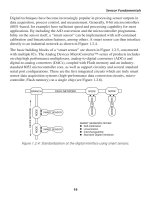
19.3 Strain Gage Sensor Installations
George C. Low, HITEC Corporation
The various types of strain gages covered elsewhere in this book can be installed by
a variety of different methods. This section will attempt to provide some detail on
each of the more popular methods of installation using the most popular strain gage
types (bonded foil resistance strain gages and free filament strain gages). The reader
is encouraged to study more about the methods that are of interest, as not all of the
intricacies of the installation techniques can be covered in this brief section. Please be
aware that there is a definite art to installing strain gages as it is primarily a manual
process, and particularly with the esoteric, free filament strain gage installations, the
quality of the installation is dependent to some degree on the installer’s experience

and is not entirely based on whether or not the proper steps were followed. There are
various modifications to the following installation techniques based on exact require-
ments, environment, etc., but these can be considered general installation technique
guidelines.
There are methods of installing strain gages in which the strain gage is actually cre-
ated during the installation process. This type of installation is commonly referred to
as vacuum depositing or sputtering. This particular installation technique is not con-
sidered part of the general strain gage installation methods and is only covered briefly
at the end of this section.
We will break down the strain gage installations into three broad categories: General
Stress Analysis, Precision Transducer Installations, and Elevated Temperature In-
stallations. The final section will be on specialty installations and will briefly make
mention of other types of installations.
General Stress Analysis Installation (Bonded Foil Strain Gage)
For general stress analysis, the user is primarily interested in obtaining stress/strain
data as fast as possible and as accurately as possible. Examples of this are FEA model
validation, general design validation, structural failure analysis, simple accelerated
life cycle testing, etc. These types of installations usually do not warrant the same
type of manufacturing methods as a high performance and high accuracy transducer
(for example, a post cure operation).
Strain Gages
523
The most common method of installation for a bonded foil resistance strain gage in
this category is using a room temperature cure cyanoacrylate adhesive consisting of a
catalyst and an adhesive. This type of installation requires a minimum amount of tools
and equipment and also a minimum amount of experience. The basic procedure is as
follows:
a. Surface preparation, either a chemical cleaning process or a combination of
fine grit abrasive and chemical cleaning. It should be noted that in some types
of tests, the surface being measured must not be altered, which dictates a

chemical cleaning only.
b. Gage location centerlines or layout lines are burnished on the part using a
method that will not cause bumps or other anomalies under the gage grid after
installation. Examples of this can be simply a pencil, a scribe tool with a brass
tip, etc. In some cases the layout lines can be applied using laser marking.
c. The gage is now carefully placed in position and held in place using a piece of
Mylar® tape. lt is sometimes desirable not to seal the strain gage coupon on
all four sides with the tape. This is to allow “squeeze out” of the adhesive and
provide a uniform bond line with no bumps or air pockets. Carefully lift back
the Mylar tape with gage adhered to the tape and fold it back over itself expos-
ing the bottom or bondable surface of the strain gage.
d. The catalyst is now applied to the gage backing, while the adhesive is applied
to the component surface.
e. Fold the gage back in place, and using thumb pressure, press and hold the
gage per the manufacturer’s recommended guidelines, usually at least one
minute.
At this point, the strain gage is bonded to the component and is ready for the next
step, which is lead wire attachment. The lead wire length and material is selected
based on the user’s test and instrumentation requirements. A suitable coating must
be installed as well in order to seal the installation from the environment and also to
provide some mechanical protection.
This is the most basic installation technique, and care must be taken when choosing
the strain gage itself. Parameters to consider include: grid length and type, backing and
foil type, resistance, self-temperature compensation rating, etc. General stress analysis
applications can also utilize the higher quality and higher capability of heat cured epoxy
adhesive systems that are more commonly utilized in transducer applications.
Chapter 19
524
Precision Transducer Installations
These installations cover a wide range of transducers, from torque transducers to

shear beams to pressure transducers. Also included in this section would be the
ever-popular component “transducerization” which includes the in-situ components
that are slightly modified to accept strain gages and they become the transducer. An
example of this is the suspension “pushrods” on an open wheel racecar. In this case,
the actual suspension pushrods have a couple pockets milled into it in which strain
gages are installed and the pushrod itself becomes a transducer that the team can use
to determine optimum suspension setup prior to a race.
These types of installations require better adhesives and routinely utilize heat cure
epoxy adhesives. Various types are available depending on operating temperature of
the transducer, surface porosity of the base transducer material, and so forth.
The general procedure, for bonded foil resistance strain gages, follows some similar
steps as the general stress analysis installations:
a. Surface preparation, usually a fine grit abrasive blast is used. Chemical clean-
ing is also required prior to the actual strain gage application in order to
ensure a contamination-free surface.
b. Gage location centerlines are burnished on the part using a method that will
not cause bumps or other anomalies under the gage grid after installation.
Examples of this can be simply a pencil, a scribe tool with a brass tip, etc. In
some cases the layout lines can be applied using laser marking.
c. The gage is now carefully placed in position and held in place using a piece
of Mylar tape. It is sometimes desirable to not seal the strain gage coupon on
all four sides with the tape. This is to allow “squeeze out” of the adhesive and
provide a uniform bond line with no bumps or air pockets. Carefully lift back
the Mylar tape with gage adhered to the tape and fold it back over itself expos-
ing the bottom or bondable surface of the strain gage.
d. The adhesive is now applied to the gage backing and the component. Allow to
air dry per the manufacturer’s recommended guidelines.
e. Fold the gage back in place, place a piece of Teflon® film over the Mylar tape,
and place a suitably sized rubber pad over the Teflon film.
Strain Gages

525
f. A critical part of the installation is using the correct clamping pressure to
clamp the gage. Each adhesive has a recommended clamping pressure for
precision transducer applications. It should also be noted that some applica-
tions require more than the recommended pressure. This author is aware
of an application that required more than twice the manufacturer’s recom-
mended clamp pressure in order to meet certain specifications such as creep
performance. The clamp should also be calibrated and of a suitable design
that allows for efficient clamping and unclamping if used for production type
work. The clamped transducer is then placed in an oven and allowed to ramp
up at a controlled rate to the desired cure temperature. A common type of
installation on a steel transducer body, for instance, would require a cure of 2
hours at 350°F.*
g. The next step in the procedure is the post cure. This is important for long-term
stable transducer operation. Allow the transducer to cool after the cure opera-
tion and remove the clamp. Place the transducer back in the oven and post
cure the transducer (with no clamp) at 50°F over either the cure temperature or
the maximum operating temperature, whichever is higher.
h. After installation, the gages are wired as appropriate, usually in a Wheatstone
bridge configuration. Further transducer manufacturing steps occur but are
outside of the scope of this section.
Elevated Temperature Installations
Installations under this category cover installations for use over about 700°F. For that
reason they require the use of free filament wire strain gages. It should also be noted
that at these higher temperatures, essentially the only measurements that can be made
with any certainty are dynamic measurements, as opposed to static. Some static mea-
surements are said to have been made up to 1200°F, but this author does not know the
accuracies and repeatability of those measurements.
The following are general procedures to be followed for free filament strain gage ap-
plications. As in the other installation categories covered, there can be variations to

this based on material requirements, experience, etc. For this type of installation in
particular, the installer’s experience and skill are critical to a quality installation that
will survive the rigors of a jet engine spin pit test, for instance.
Chapter 19
526
These strain gages can be installed using two different methods, either using ceramic
cement, or via a ROKIDE® flame spray process. Ceramic cement is usually utilized
for applications below 1200°F, where the use of the flame spray process would pro-
vide unwanted reinforcement to a thin specimen, and also where the installer cannot
spray due to space constraints. The ROKIDE process provides better erosion char-
acteristics over ceramic cement but does not perform as well in fatigue as ceramic
cements do. ROKIDE is essentially aluminum oxide and comes in various purity
levels.
The basic procedures are as follows:
Ceramic Cement Process
This process utilizes ceramic cement which, when applied in the appropriate steps,
ultimately encapsulates the free filament strain gage grid in ceramic cement, which
protects the strain gage from the harsh elevated temperature environment.
a. Where possible, pre-bake the component to eliminate any surface oils, etc.
b. Carefully burnish the surface of the component extending the lines beyond the
area to be grit blasted. This area would include the entire area where the strain
gage grid is applied as well as the lead wire routing areas that require ceramic
cement application.
c. Mask the component with tape for the gage locations and lead wire paths. Grit
blast using a pressure blaster using new grit of suitable size for the particular
component.
d. Remove all tape and inspect for contaminants.
e. Mask the outline of the gage location and lead wire routing areas with Mylar
tape. Apply a pre-coat of ceramic cement per manufacturer’s guidelines to
both areas. After the cement has air dried for a nominal length of time, remove

the Mylar tape. Oven cure the pre-coat per manufacturer’s guidelines.
f. The strain gages themselves come from the manufacturer on a slide with inte-
gral mastic, which holds the gage shape. Carefully remove the gage from the
manufacturer’s slide and position the gage over the correct gage location.
g. Carefully press the mastic into contact with the pre-coat using fine-tipped
tweezers or other suitable tool.
Strain Gages
527
h. Using a clean brush, apply ceramic cement in thin layers over the exposed grid
and lead wires in between the tape bars. Allow to air dry and place in an oven
for cure per the manufacturer’s guidelines.
i. Verify the gage resistance and remove the remaining tape bars.
j. Apply a thin layer of ceramic cement over the newly exposed areas of the grid
and lead wires. Allow to air dry and place in an oven for cure per the manufac-
turer’s guidelines.
k. Once all lead wires have been attached, perform final electrical inspection by
checking the resistance of the circuit, as well as the insulation resistance.
l. A typical ceramic cement installation of this type is between 0.007″ to 0.008″
thick.
ROKIDE Flame Spray Process
This process utilizes a special spray gun which, using oxygen and acetylene and the
appropriate grade of ROKIDE rod, sprays a molten ceramic onto the desired surface.
This ultimately encapsulates the strain gage grid and protects it from the harsh elevat-
ed temperature environment.
a. Where possible, pre-bake the component to eliminate any surface oils, etc.
b. Carefully burnish the surface of the component extending the lines beyond
the area to be grit blasted. This area would include the entire area where the
strain gage grid is applied as well as the lead wire routing areas that require
ROKIDE flame spray application.
c. Mask the component with suitable tape for the gage locations and lead wire

paths. Grit blast using a pressure blaster using new grit of suitable size for the
particular component. Clean with dry, contamination-free air.
d. Apply a thin nickel aluminide base coat. The nickel aluminide retards oxi-
dation and also provides a better mechanical bond for the aluminum oxide
(ROKIDE). Clean with dry, contamination-free air.
e. Apply a thin aluminum oxide pre-coat, which will electrically insulate the free
filament strain gage from the component surface. Clean with dry, contamina-
tion-free air.
f. The strain gages themselves come from the manufacturer on a slide with inte-
gral mastic, which holds the gage shape. Carefully remove the gage from the
manufacturer’s slide and position the gage over the correct gage location.
Chapter 19
528
g. Carefully press the mastic into contact with the pre-coat using fine-tipped
tweezers or other suitable tool. Ensure the gage grid is not pressed too hard so
as to conform it to the aluminum oxide pre-coat.
h. Box in the gage grid by placing tape around the perimeter of the grid using
suitable high temperature tape. This ensures that only a minimum amount of
surface area will be covered by the aluminum oxide, which does cause a rein-
forcing effect.
i. Apply a light aluminum oxide tack-coat to the exposed gage grid and gage
leads. Always take resistance readings throughout the process to ensure the
gage grid has not become damaged.
j. Remove the perimeter tape first, and then the tape bars which were originally
holding the strain gage grid to the aluminum oxide pre-coat.
k. Box in the installation again using the same tape as in the previous operation.
This second application of perimeter tape should be positioned about 1/32″
beyond the first tape application. This will provide a layering effect, which
will minimize the sharp edge of the final aluminum oxide installation.
l. Spray the final coat of aluminum oxide over the entire strain gage and strain

gage leads as
appropriate.
m. Remove all tape and inspect for circuit resistance and insulation resistance.
n. A typical ROKIDE installation of this type is generally about 0.012″ thick.
Other Installation Methods
One unique method of strain gage installation requires specialized manufacturing
equipment and technical knowledge. This is referred to as sputtering or vacuum
deposition. During this process the strain gage itself is created during the installation
process. It is beyond this scope of this section to address this specialized method of
installation.
Another specialized method is called thick film, which again is outside of the scope of
this section.
These two methods are considered specialized and have been covered in the relevant
section of the strain sensor chapter. In general they do not cover nearly as broad a
range of applications as the three sections broken out above; therefore more attention
has been given to the more common installations.
Strain Gages
529
Another strain gage installation technique lends itself to higher volume applications
(usually 10,000 pieces and higher). Assuming the flexure to be gaged is essentially
flat, the flexures can be arranged in an array. This can be either as part of the manufac-
turing process as in chemical milling of thin cantilever/bending beams in a sheet, or
can be separate flexures arranged in an array via appropriate manufacturing fixtures.
The actual strain gage application is performed by bonding an entire sheet of gages
(strain gages also in an array form that have not yet been separated into individual
pieces) to the flexures. The array is then subject to clamping pressures using a press
type setup. The gaged flexures are then trimmed and separated from each other and
the result is an efficiently gaged batch of beams.
A twist to this process is when the strain gage foil is bonded to the backing, which is
in turn bonded to the flexure all in one operation. The composite is then etched at the

same time; i.e., the strain gage pattern as well as the flexure is created during the same
operation. This, of course, only lends itself to the thin (<0.1″) beam type flexures.
A weldable strain gage installation is yet another form of installation. This type of
gage comes from the manufacturer as a complete assembly consisting of a metal
shim, a strain gage, lead wires, and potting/coating, completely bonded and assem-
bled. The potting/coating is an appropriate compound suitable for the environment.
Weldable strain gages come in both high temperature and room temperature versions.
These gages are applied to the surface of the component to be tested using spot-weld-
ing techniques. Weldable strain gages are essentially only used in the field in areas
where more standard strain gages cannot be installed due to either installer’s skill or in
locations where it is impossible to perform any other type of strain gage installation.
The general techniques and processes listed in this section should not be considered
the final word on strain gage installations. As mentioned previously, there are many
different variations to these processes based on operating environment, size of the
component or transducer, materials being used, and so forth. In all cases, it is impera-
tive the installer read all instructions for the installation materials being utilized. The
precision transducer processes, for example, can be used for installing semiconductor
strain gages, although some steps need to be altered such as clamping pressure, etc.
The basic process, however, is very similar.
This page intentionally left blank
531
C H A P T E R
20
Temperature Sensors
John Fontes, Senior Applications Engineer, Honeywell Sensing and Control
Because temperature can have such a significant effect on materials and processes
at the molecular level, it is the most widely sensed of all variables. Temperature is
defined as a specific degree of hotness or coldness as referenced to a specific scale. It
can also be defined as the amount of heat energy in an object or system. Heat energy
is directly related to molecular energy (vibration, friction and oscillation of particles

within a molecule): the higher the heat energy, the greater the molecular energy.
Temperature sensors detect a change in a physical parameter such as resistance or
output voltage that corresponds to a temperature change. There are two basic types of
temperature sensing:
■ Contact temperature sensing requires the sensor to be in direct physical
contact with the media or object being sensed. It can be used to monitor the
temperature of solids, liquids or gases over an extremely wide temperature
range.
■ Non-contact measurement interprets the radiant energy of a heat source in the
form of energy emitted in the infrared portion of the electromagnetic spec-
trum. This method can be used to monitor non-reflective solids and liquids but
is not effective with gases due to their natural transparency.
20.1 Sensor Types and Technologies
Temperature sensors comprise three families: electro-mechanical, electronic, and resis-
tive. The following sections discuss how each sensor type is constructed and used to
measure temperature and humidity.
Electro-mechanical
Bi-metal thermostats are exactly what the name implies: two different metals bond-
ed together under heat and pressure to form a single strip of material. By employing
the different expansion rates of the two materials, thermal energy can be converted
into electro-mechanical motion.
Chapter 20
532
There are two basic bi-metal thermostat technologies: snap-action and creeper. The
snap-action device uses a formed bi-metal disc to provide a near instantaneous change
of state (open to close and close to open). The creeper style uses a bi-metal strip to
slowly open and close the contacts. The opening speed is determined by the bi-metal
selected and the rate of temperature change of the application.
Bi-metal thermostats are also available in adjustable versions. By turning a screw, a
change in internal geometry takes place that changes the temperature setpoint.

Bulb and capillary thermostats make use of the capillary action of expanding or
contracting fluid to make or break a set of electrical contacts. The fluid is encap-
sulated in a reservoir tube that can be located 150mm to 2000mm from the switch.
This allows for slightly higher operating temperatures than most electro-mechanical
devices. Due to the technology involved, the switching action of these devices is slow
in comparison to snap-action devices.
Electronic
Silicon sensors make use of the bulk electrical resistance properties of semiconduc-
tor materials, rather than the junction of two differently doped areas. Especially at
low temperatures, silicon sensors provide a nearly linear increase in resistance versus
temperature or a positive temperature coefficient (PTC). IC-type devices can provide a
direct, digital temperature reading, so there’s no need for an A/D converter.
Infrared (IR) pyrometry. All objects emit infrared energy provided their temperature
is above absolute zero (0 Kelvin). There is a direct correlation between the infrared
energy an object emits and its temperature.
IR sensors measure the infrared energy emitted from an object in the 4–20 micron
wavelength and convert the reading to a voltage. Typical IR technology uses a lens to
concentrate radiated energy onto a thermopile. The resulting voltage output is ampli-
fied and conditioned to provide a temperature reading.
Factors that affect the accuracy of IR sensing are the reflectivity (the measure of a
material’s ability to reflect infrared energy), transmissivity (the measure of a materi-
al’s ability to transmit or pass infrared energy), and emissivity (the ratio of the energy
radiated by an object to the energy radiated by a perfect radiator of the surface being
measured).
An object that has an emissivity of 0.0 is a perfect reflector, while an object with an
emissivity of 1.0 emits (or absorbs) 100% of the infrared energy applied to it. (An
emissivity of 1.0 is called a “blackbody” and does not exist in the real world.)
Temperature Sensing
533
Thermocouples are formed when two electrical conductors of dissimilar metals or

alloys are joined at one end of a circuit. Thermocouples do not have sensing elements,
so they are less limited than resistive temperature devices (RTDs) in terms of materi-
als used and can handle much higher temperatures. Typically, they are built around
bare conductors and insulated by ceramic powder or formed ceramic.
All thermocouples have what are referred to as a “hot” (or measurement) junction and
a “cold” (or reference) junction. One end of the conductor (the measurement junction)
is exposed to the process temperature, while the other end is maintained at a known
reference temperature. (See Figure 20.1.1.) The cold junction can be either a refer-
ence junction that is maintained at 0°C (32°F) or at the electronically compensated
meter interface.
Figure 20.1.1: Thermocoupler.
Source: Desmarais, Ron and Jim Breuer. “How to Select and Use the Right Temperature Sensor.”
Sensors Online. January 2001. />When the ends are subjected to different temperatures, a current will flow in the wires
proportional to their temperature difference. Temperature at the measurement junction
is determined by knowing the type of thermocouple used, the magnitude of the mil-
livolt potential, and the temperature of the reference junction.
Thermocouples are classified by calibration type due to their differing voltage or EMF
(electromotive force) vs. temperature response. The millivolt potential is a function of
the material composition and conductor metallurgical structure. Instead of being as-
signed a value at a specific temperature, thermocouples are given standard or special
limits of error covering a range of temperature.