A Principles of Hyperplasticity Part 6 doc
Bạn đang xem bản rút gọn của tài liệu. Xem và tải ngay bản đầy đủ của tài liệu tại đây (576.38 KB, 25 trang )
110 6 Advanced Plasticity Theories
when these two surfaces come in contact with each other. The modulus can, for
instance, be specified by an expression of the form,
0
0
hH hH
J
§·
G
G
¨¸
G
©¹
(6.8)
where as before
PR
G
is the distance from the current stress point to the image
point. The form ensures that
0hH and
00
hhG . This formulation is very
close in concept to bounding surface plasticity.
This form of plasticity, however, avoids the problem inherent in the bounding
surface models of ratcheting for small cycles of unloading and reloading. The
more sophisticated rules for defining the image point and the translation of the
inner yield surface provide a more realistic way for describing hysteretic behav-
iour and the effect of past loading history.
This process can be taken a step further by introducing a set of nesting sur-
faces within the domain between
0f and
0F
. These surfaces can translate
and expand or contract due to plastic straining. They are capable of encoding in
a more subtle way the details of the past stress history. The relative motion be-
tween each adjacent surface is defined by rules similar to (6.6) to ensure that
they remain nested. The hardening modulus can be defined by an interpolation
formula such that it is
0
h on the innermost yield surface, and equal to H on the
outermost surface. For instance, it can be assumed if the stress point is in con-
tact with n surfaces out of a total of N:
0
1
Nn
hH h H
N
J
§·
¨¸
©¹
(6.9)
The configuration of the nesting surfaces and therefore the subsequent stiff-
ness for a particular stress path depends on the past history of loading. The ma-
terial response for any loading history may be studied by following the evolution
of the configurations of the nested surfaces. This model possesses a multi-level
memory structure because, for cyclically varying stress, only a certain number of
surfaces undergo translation; the other surfaces may change only isotropically.
This approach can be extended to an infinite number of surfaces, although for
practical computations, a finite number is necessary.
6.4 Multiple Surface Plasticity
Although it has certain advantages, the translation rule for multiple yield sur-
faces that requires that the surfaces remain nested is not strictly necessary (see
Section 6.5). The principal advantage of the nested approach is that this allows
the determination of a single plastic strain component, with its magnitude estab-
lished by one of the above procedures for the hardening modulus.
6.4 Multiple Surface Plasticity 111
An alternative approach is to introduce multiple yield surfaces, but to treat
each as independent, giving rise to a separate plastic strain component. The total
strain is the sum of the elastic strain and the plastic strain components:
1
N
epn
ij
ij ij
n
H H H
¦
(6.10)
Each yield surface is specified in the form
ıİ,0
pn
n
ij
ij
f
, where for
simplicity the yield surface depends only on the plastic strains associated
with that surface, and is not coupled to other yield surfaces by dependence
on their plastic strains. In principle, non-associated flow can be specified read-
ily by defining plastic potentials distinct from the yield surfaces so that
n
pn
n
ij
ij
gw
H O
wV
.
Combining the elasticity relationship and the flow rule, one obtains:
ıİ
ı
1
n
N
n
ij ijkl kl
ij
n
g
d
§·
w
¨¸
O
¨¸
w
©¹
¦
(6.11)
and the plastic multipliers are eliminated by the consistency conditions for each
of the yield surfaces:
0
nn nnn
pn
n
ij ij
ij
pn pn
ij ij ij
i
j
i
j
ff ffgww www
V H V O
wV wV wV
wH wH
(6.12)
The analysis proceeds exactly as for the single surface model with the elastic-
plastic matrix determined as
1
nn
ijab mnkl
N
ep
ab mn
ijkl
ijkl
nn
n
pqrs
pn
pq rs
rs
gf
dd
dd
f
fg
d
½
ww
°°
°°
wV wV
°°
®¾
§·
°°
www
¨¸
°°
¨¸
wV wV
wH
°°
©¹
¯¿
¦
(6.13)
Strictly, the summations in the above equations are only for the “active” yield
surfaces, for which
0
n
f
; on the other surfaces, simply,
0
n
O
.
It can be seen that the multiple surface method is simpler in concept than the
nested surface method. It does not involve the plethora of ad hoc rules about
translation and hardening of the inner surface, most of which are introduced
simply to guarantee “nesting” rather than to reproduce any well-defined feature
of material behaviour. The multiple surface models do, however, have all the
advantages of nested surface models in modelling hysteresis and stress history
effects. An example of this type of model was given by Houlsby (1999).
This approach, too, can be extended to an infinite number of surfaces.
112 6 Advanced Plasticity Theories
6.5 Remarks on the Intersection of Yield Surfaces
6.5.1 The Non-intersection Condition
The use of kinematic hardening plasticity with multiple yield surfaces has a his-
tory of more than 30 years. It has proved a very convenient framework for mod-
elling the pre-failure behaviour of soils and other materials, allowing a realistic
treatment of issues such as non-linearity at small strain and the effects of recent
stress history. The growing interest in modelling small strain behaviour of soils
has recently resulted in the development of many so-called “bubble” models,
such as those described by Stallebrass and Taylor (1997), Kavvadas and Amorosi
(1998), Rouainia and Muir Wood (1998), Gajo and Muir Wood (1999), Houlsby
(1999), Puzrin and Burland (2000), and Puzrin and Kirshenboim (1999).
In all the above models, except Houlsby (1999), the “translation rules” are
specified to avoid intersection of the yield surfaces, and it is commonly believed
that this non-intersection condition must be met, but some publications express
a contrary view.
This subject is discussed here because the non-intersection condition leads to
unnecessary complications in kinematic hardening hyperplasticity with multiple
yield surfaces. As discussed above, the simple translation rules used by Ziegler or
Prager correspond to simple forms of Gibbs free energy. If non-intersection is to be
imposed, much more complex energy expressions are required, in which terms
involving cross-coupling between different plastic strain components must appear.
Puzrin and Houlsby (2001a) argue that the condition is not necessary, but is
required only when an incrementally bilinear constitutive law is to be derived.
Sometimes it is claimed that, even if not strictly necessary, the non-intersection
condition should be accepted on pragmatic grounds. Incremental bilinearity
(and hence non-intersection) certainly offers some advantage in computation.
The main one is that, if an updated stiffness approach is taken in finite element
analysis, the incremental stress-strain relationship is known (for plastic load-
ing), reducing the need for iteration. At the opposite extreme, if an incremen-
tally non-linear approach (e.
g. as in hypoplastic theories) is used, the incre-
mental stress-strain relationship cannot be determined without prior knowledge
of the path during the increment. If intersection of yield surfaces is allowed, an
intermediate case occurs: the response is incrementally multilinear (see the
discussion below). In practice, this does not prove to be a significant disadvan-
tage, since for most relatively smooth stress paths, the incremental plastic re-
sponse can be determined in advance for each increment.
6.5.2 Example of Intersecting Surfaces
To demonstrate that the non-intersection condition is not strictly necessary, we
describe here a model with two yield surfaces that are allowed to intersect. It will
6.5 Remarks on the Intersection of Yield Surfaces 113
be seen that this model poses no theoretical difficulties. Consider the plasticity
model with two kinematic hardening yield surfaces in a two-dimensional stress
space, as shown in Figure 6.3. The yield surfaces are
2
11 1
1
2
22 2
2
0
0
T
T
fk
fk
V U V U
V U V U
(6.14)
where
^
`
12
,
T
VVV
is the stress vector;
^
`
ȡȡ
11
1
12
,
T
U
and
^
`
ȡȡ
22
2
12
,
T
U
are the coordinates of the centres of the yield surfaces, and
1
k and
2
k are their radii. Plastic yielding and hardening are calculated using an
associated flow rule:
ȜȜ
ȜȜ
1
1
111
2
2
222
2
2
p
p
f
f
w
w
w
w
H V U
V
H V U
V
(6.15)
V
1
V
2
V
'
U
(1)
U
(2)
F
(1)
F
(2)
Figure 6.3. Two-dimensional kinematic hardening plasticity model
114 6 Advanced Plasticity Theories
where
1
O
and
2
O
are non-negative multipliers;
^
`
İİ
111
12
,
T
p
pp
H
and
^
`
İİ
222
12
,
p
pp
H
are the plastic strain vectors associated with each of the sur-
faces, so that the total plastic strain vector is given by
12
p
pp
H H H
.
Plastic hardening is calculated using Prager’s translation rule (which in this
case is identical to Ziegler’s):
1
1
1
p
E
U H
(6.16)
and
2
2
2
p
E
U H
(6.17)
Finally, the elastic component of this model is defined by
e
E V H , where
^
`
12
,
T
eee
H HH
is the elastic strain vector, so that the total strain vector is given
by
ep
H H H
.
The model defined by Equations (6.14)–(6.17) is a particular case of the
multi-surface model (7.38)–(7.39) which will be derived in Section 7.5 within the
hyperplastic framework.
Prager’s and Ziegler’s translation rules are known to violate the non-
intersection condition. Consider as an example the case presented in Figure 6.4.
During loading, the stress state P was reached, where the two surfaces touch
each other (if they do not touch at only one point, they intersect and the proof is
completed). Next a stress reversal took place and the stress state moved inside
the yield surface
1
f
such that the current stress state
V
was reached, which is
on this yield surface but not on the outer yield surface. The next stress incre-
ment
dV
is such that plastic response of the yield surface
1
f
will occur, and
will cause a strain increment
1
p
dH
directed along the vector
11
F V U
, as
prescribed by the associated flow rule (6.15). Then, according to Prager’s trans-
lation rule (6.17), the instantaneous displacement
1
dU
of the centre Q of the
yield surface
1
f
will also be directed along the vector
11
F V U
. There-
fore, if the current stress state
V
is located so that the angle
D
between the
vectors
F and
1
U
is acute, the instantaneous displacement vector
1
dU
will
have a component directed along the ray QP. In this case, when the stress in-
crement
dV
takes place, the point P on the yield surface
1
f
moves into the
exterior of the yield surface
2
f
, and the surfaces intersect.
6.5 Remarks on the Intersection of Yield Surfaces 115
V
1
V
2
D
U
(1)
F
(1)
d
V
P
Q
O
V
Figure 6.4. Example of a violation of the non-intersection condition
6.5.3 What Occurs when the Surfaces Intersect?
There are no significant detrimental effects when yield surface intersect, pro-
vided that the plastic loading and consistency conditions are applied separately
to each yield surface [see, for example, de Borst (1986)]. In this case, the consti-
tutive relationship simply becomes multilinear instead of bilinear.
Consider, for example, the kinematic hardening model with two yield sur-
faces described by Equations (6.14)–(6.17). The incremental stress-strain re-
sponse of this model is derived by applying consistency conditions
1
0f
and
2
0f
separately to each surface as appropriate. For this case, the following
incremental relationships can be obtained:
ȜȜ
1122
22
E
V
H V U V U
(6.18)
where
Ȝ
1
1
1
2
11
1
, when 0
2
0, when 0
T
f
Ek
f
°
°
®
°
°
¯
V U V
(6.19)
116 6 Advanced Plasticity Theories
V
1
V
2
O
Zone 1
Zone 3
Zone 4
Zone 2
Figure 6.5. Intersecting yield surfaces
Ȝ
2
2
2
2
22
2
, when 0
2
0, when 0
T
f
Ek
f
°
°
®
°
°
¯
V U V
(6.20)
and
are Macaulay brackets (i.
e. ,0; 0,0xxx x x ! d).
Assuming that the surfaces intersect at the current stress state in Figure 6.5,
four different types of behaviour are encountered, depending on which of the
four possible zones the incremental stress vector is directed into.
Zone 1:
Ȝ
Ȝ
1
1
1
2
2
11
2
2
2
22
0
0
T
T
E
Ek
Ek
!
°
®
°
!
¯
V U V
V
H V U
V U V
V U
(6.21)
Zone 2:
Ȝ
Ȝ
1
1
1
2
2
11
0
0
T
E
Ek
!
°
®
°
d
¯
V U V
V
H V U
(6.22)
6.6 Alternative Approaches to Material Non-linearity 117
Zone 3:
Ȝ
Ȝ
2
1
2
2
2
22
0
0
T
E
Ek
d
°
®
°
!
¯
V U V
V
H V U
(6.23)
Zone 4:
Ȝ
Ȝ
1
2
0
0
E
d
°
®
°
d
¯
V
H
(6.24)
Equations (6.21)–(6.24) represent an example of an incrementally multilinear
constitutive relationship, as opposed to a bilinear one obtained when the non-
intersection condition is satisfied. During loading, zones 2 and 3 would be en-
countered only in rather rare circumstances which would involve rather con-
torted stress paths. Many other recent developments in generalised plasticity,
hypo-, and hyperplasticity are based on the use of incrementally non-linear and
multilinear constitutive relationships.
The main conclusion is that the non-intersection condition is necessary only
when a bilinear constitutive law has to be derived. Intersection of yield surfaces,
when treated properly, leads to multilinear constitutive relationships, which are
consistent with recent developments in plasticity theory.
Note that we make no case here that every model that allows intersection of
yield surfaces may be theoretically consistent. It would be quite possible to for-
mulate such a model so that it was either theoretically unacceptable or produced
unjustifiable results. The case we present is simply that intersection of yield
surfaces is allowable and on occasions may offer advantages.
6.6 Alternative Approaches to Material Non-linearity
Plasticity theory is not the only method that has been used to model the irre-
versible and non-linear behaviour of rate-independent materials. For complete-
ness, two further alternatives should be mentioned.
Endochronic theory [Valanis (1975); Bazant (1978)] enjoyed some popularity
at one time, but has now largely fallen into disuse. Initially it was an attempt to
model irreversibility within a thermodynamic context and without recourse to
yield surfaces. It concentrated instead on the use of an “intrinsic time”, which
was typically identified with some measure of plastic strain. Incremental rela-
tions relating stresses, strains, and intrinsic time increment were proposed.
Unfortunately, the main purpose of endochronic theory – to avoid yield surfaces
– was the cause of its downfall. Real materials that exhibit rate-independent,
irreversible behaviour also exhibit the phenomenon of a yield surface. Thus it
became necessary to modify endochronic theory to include yield surfaces artifi-
cially. The theories became increasingly contrived, and are now rarely used.
Hypoplasticity is closely related to endochronic theory, although it does not
employ an intrinsic time. Instead, rate equations are proposed specifying the
118 6 Advanced Plasticity Theories
stresses in terms of the strain rates. These equations make much use of tensor
analysis to identify the most general forms of first-order (but not necessarily
linear) expressions for stress rate in terms of strain rate. For example, Kolymbas
(1977) assumes a direct incrementally non-linear stress-strain relationship:
ij ijkl kl ij kl kl
LNV H HH
(6.25)
where
ijkl
L and
ij
N are linear operators. The early theories did not use yield
surfaces, but (for the same reasons as encountered by endochronic theory) more
recent theories have become increasingly complex to introduce the phenome-
non of yield surfaces. The theories are still popular in some quarters, but in our
view are unlikely to find long-term favour.
6.7 Comparison of Advanced Plasticity Models
As seen from the above examples of different plasticity formulations, their com-
mon feature is the existence of an outer or bounding surface
0F
(in soils of-
ten defined by the degree of material consolidation). In classical plasticity strain
hardening models, this surface is assumed to be a yield surface, containing an
entirely elastic domain. To incorporate plastic flow within this surface, bound-
ing surface models, nested surface models, and multiple surface models have
been developed.
In bounding surface models, the
0F
surface is treated as a bounding sur-
face, and a loading surface passing through the current stress state is defined
using a specific mapping rule. This mapping rule also defines the distance in the
stress space between the stress state and the bounding surface, and the postu-
lated hardening rule depends on this distance. The disadvantage of these models
is the unrealistic “ratcheting” behaviour for small unload-reload cycles.
In nesting surface models, the stress history of cyclic loading may be fol-
lowed, and the ratcheting problem avoided by the more sophisticated rules for
the evolution of the surfaces. Unfortunately, a number of ad hoc assumptions
have to be introduced specifying the motion of the surfaces. True multiple sur-
face models (without the nesting requirement) avoid these assumptions, and are
simpler in concept than nested surface models. They can accommodate non-
associated flow more easily. They too have a disadvantage. Since each surface
acts independently, each must be checked for yield, whilst for nested surface
models, it is known that the surfaces are engaged in order from the innermost to
the outermost. All multiple surface models can in principle be extended to an
infinite number of surfaces.
There is no definitive choice between the more sophisticated plasticity mod-
els. In the following, however, we shall develop hyperplasticity versions of mul-
tiple surface models. It will be seen that these then lead naturally to a further
extension into models with an infinite number of surfaces.
Chapter 7
Multisurface Hyperplasticity
7.1 Motivation
The purpose of this chapter is to present a more general framework for hyper-
plastic modelling of the kinematic hardening of plastic materials. In Sec-
tion 5.4.3, a simple example of a single kinematically hardening yield surface
was presented. The elastoplastic stress-strain behaviour of this simple model
was bilinear. The stiffness is controlled by elastic moduli within the yield surface
and by the hardening moduli at the surface. The limitations of this simple model
become clear when its behaviour is compared to that of some real materials, in
particular soils. In soils, the true linear elastic region is often negligibly small,
and plastic yielding starts almost immediately with straining. The behaviour
therefore appears to be highly non-linear even within the large-scale yield sur-
face. It also appears that soil has a memory of stress-reversal history within the
large-scale yield surface. A simple single surface kinematic hardening model
cannot simulate these features.
In an attempt to solve this problem, Iwan (1967) and Mroz (1967) introduced
the concept of multiple yield (or loading) surfaces, as discussed in Chapter 6. In
multiple yield surface kinematic hardening models, the size of the true linear
elastic region can be reduced, even to the limiting case in which it vanishes com-
pletely. The stress-strain behaviour becomes piecewise linear and can follow
more closely the true non-linearity of the material. Importantly, the model has
a discrete memory of stress reversals, reflected in the relative configuration of
the yield surfaces. Generalization of the multiple surface concept to an infinite
number of yield surfaces produces models with a continuous field of yield sur-
faces. These models allow the simulation of the true non-linear stress-strain
behaviour and a continuous material memory, and will be the subject of Chap-
ter 8.
120 7 Multisurface Hyperplasticity
7.2 Multiple Internal Variables
For simplicity, in Chapter 4, we considered materials which could be character-
ised by a single kinematic internal variable
ij
D , which was in the form of a sec-
ond-order tensor. The kinematic internal variable can often be conveniently
identified with the plastic strain. The significance of the single internal variable
is that a single yield surface is derived, on which there is an abrupt change from
elastic to elastic-plastic behaviour. The generalisation of the results to some
other cases is straightforward; for instance, a scalar internal variable can be
obtained simply by dropping the subscripts from the variables
ij
D ,
ij
F , and
ij
F
in Chapter 4.
The generalisation to some more complex cases is marginally more complex.
For instance, N second-order tensor internal variables would mean that the
function for the Gibbs free energy
,,
ij ij
g VDT
in Chapter 4 is simply general-
ised to
1
,,, ,
N
ij
ij ij
g VD D T!
. The corresponding differential
ij
ij
g
w
F
wD
is
replaced by
n
ij
n
i
j
g
w
F
wD
where
1nN !
. The corresponding forms and re-
sults for other energy functions and differentials follow a similar pattern. When
Legendre transformations are made between different functions, the number of
possible transformations becomes enormous (for instance, there are
2
2
N
possible forms of the energy function). However, it is likely that only a small
fraction of the possible forms would be of practical application, and so no sys-
tematic presentation of the forms with multiple internal variables is given here.
If any of the N
internal variables are scalars rather than tensors, then all that
is necessary is to drop the subscripts from the appropriate variables.
The main reason for the introduction of multiple internal variables is to allow
the definition of models with multiple yield surfaces. These can be used for
a variety of purposes,
e.
g.:
x modelling separately compression and shear effects, as may be appropriate
for some granular materials (
i.
e. “cone and cap” models);
x modelling anisotropy by using multiple kinematically hardening yield sur-
faces;
x modelling the memory of stress reversals; and
x approximation of a smooth transition from elastic to plastic behaviour.
The last of these purposes is perhaps the most important. The use of internal
variables (within the thermodynamic framework) is an extremely powerful
method for describing the past history of an elastic-plastic material, but suffers
from the disadvantage that it inevitably leads to abrupt changes between elastic
and elastic-plastic behaviour. Although using multiple internal variables allows
these changes to be divided into a number of smaller steps, a completely smooth
7.3 Kinematic Hardening with Multiple Yield Surfaces 121
transition can be achieved only by introducing an infinite number of internal
variables. Such an idea leads to the concept of an internal function rather than
internal variables. The generalisation of the results given in Chapter 4 to internal
functions is rather more complex than the generalisations to multiple variables
discussed above and will be the subject of Chapter 8.
7.3 Kinematic Hardening with Multiple Yield Surfaces
7.3.1 Potential Functions
The model with a single yield surface presented in Section 5.4.3 can be extended
to multiple yield surfaces by modifying the two potential functions that define
the constitutive behaviour. The specific Gibbs free energy becomes a function of
the stress and a finite number of internal variables
,1,,
n
ij
nND !
, where N
is the total number of the yield surfaces. We choose the Gibbs free energy in the
following form:
1
1
2
11
,,,
NN
Nnnn
ij ij ij
ij ij ij ij
nn
gg g
VD D V V D D
¦¦
!
(7.1)
The dissipation function also becomes a function of the finite number of inter-
nal variables and their rates
,1,,
n
ij
nND
!
:
11
1
1
,,, ,,,
,,, , 0
NN
g
ij
ij ij ij ij
N
Nn
gn
ij
ij ij ij
n
d
d
VD D D D
VD DDt
¦
!!
!
(7.2)
where we assume that the dissipation can be decomposed into additive terms
involving each individual plastic strain tensor. For a rate-independent material,
the dissipation is a homogeneous first-order function of the plastic strain rate
tensor. For associated plasticity, the dissipation function is independent of the
stress. We shall consider only such cases in the remainder of this chapter, and so
we drop the dependence on
ij
V
in Equation (7.2).
7.3.2 Link to Conventional Plasticity
In the conventional formulation of multiple surface kinematic hardening plas-
ticity, calculation of incremental stress-strain response requires the equations to
be defined explicitly for all the yield surfaces. Then, for each yield surface, the
following rules are specified:
122 7 Multisurface Hyperplasticity
x the flow rule (or more usually the plastic potential function),
x the strain hardening rule,
x the translation rule.
All these equations and the resulting incremental stress-strain response can
be derived from the potentials (7.1) and (7.2) using Legendre transformations
and their properties for active and passive variables (see Appendix C).
The yield function is related to the dissipation function (7.2) by the Legendre
transform, where the rate of each internal variable
n
ij
D
is interchanged with the
corresponding dissipative generalised stress
,1,,
n
ij
nNF !
:
11 1
,, , ,, ,, ,
NN Nn
gn
g
ij ij ij ij ij ij ij
n
ij
nn
ij ij
ddwD DD D w D DD
F
wD wD
!! !
(7.3)
This transformation is a degenerate special case of the Legendre transformation
because the dissipation is homogeneous and first order in the rates. Therefore,
for each
1, ,nN ! ,
0
nn
ngn gn
ij ij
ydO FD
(7.4)
where
1
,, , 0
Nn
gn gn
ij ij ij
yy DDF !
is the nth yield function and
n
O
is
an arbitrary non-negative multiplier. As seen from Equations (7.4), all N yield
functions are contained in the equation of the dissipation function (7.2) in
a compact form.
The Gibbs free energy function (7.1) allows the definition of the strain tensor:
12
1
1
,,,,
N
N
ij
ij ij ij
ij
n
ij
ij
ij ij
n
g
g
wVD D D
wV
H D
wV wV
¦
!
(7.5)
where we see that the sum of the internal variables
1
N
n
ij
n
D
¦
plays exactly the
same role as the conventionally defined plastic strain
p
ij
H
and each individual
internal variable
n
ij
D
can be interpreted as a component of plastic strain associ-
ated with the plastic flow on the nth yield surface. It is also convenient to define
the elastic strain
1
e
ij
ij
gH wwV
.
The flow rule for the nth yield surface is obtained from the properties of the
Legendre transformation (7.4):
1
,, ,
,1,,
Nn
gn
ij ij ij
n
n
ij
n
ij
y
nN
wDDF
D O
wF
!
!
(7.6)
7.3 Kinematic Hardening with Multiple Yield Surfaces 123
We restricted the dissipation function to exhibit no explicit dependence on
the true stresses, so it follows that the normality represented by Equations (7.6)
in generalised stress space also holds in true stress space.
The dependence of the dissipation function on internal variables
n
ij
D
is
transferred to each yield function by the Legendre transformation (7.4) with
n
ij
D
a passive variable. Therefore, the strain hardening rule is obtained auto-
matically through the functional dependence of the yield function on plastic
strains
n
ij
D
. We shall limit our analysis here to materials with a dissipation
function (and hence yield functions) independent of internal variables
n
ij
D
, i.
e.
to materials undergoing pure kinematic hardening.
The generalised stress is defined by differentiating the Gibbs free energy func-
tion with respect to the internal variable:
12
2
,,,,
,1,,
Nnn
ij
ij ij ij ij
n
ij
ij
nn
ij ij
gg
nN
wVD D D w D
F V
wD wD
!
!
(7.7)
It is convenient at this stage to introduce the “back stress” associated with each
internal variable that is simply defined as the difference between the true and
generalised stress. By applying Ziegler’s orthogonality principle (in the form
() ()nn
ij ij
F F
), the “back stress”
n
ij
U
can be expressed as
2
,1,,
nn
ij
nn n
ij
ij ij ij
n
ij
g
nN
wD
UD VF }
wD
(7.8)
which, after differentiation for the nth yield surface, gives
wD
UD VF D
wD wD
!
2
2
,1,,
nn
ij
nn n n
ij
ij ij ij
kl
nn
ij
kl
g
nN
(7.9)
As in conventional plasticity,
U
n
ij
defines the coordinates of the centre of the nth
yield surface in true stress space. Equation (7.9) can therefore be interpreted as
the translation rule for the nth yield surface.
7.3.3 Incremental Response
In a similar way to the description of the incremental response of a hyperplastic
material with a single yield surface, two possibilities exist for each of the N yield
124 7 Multisurface Hyperplasticity
surfaces. If the material state is within the nth yield surface
0
n
gn
ij
y
§·
F
¨¸
©¹
,
then no dissipation occurs and
0
n
O
. If the material point lies on the yield
surface
0
n
gn
ij
y
§·
F
¨¸
©¹
, then plastic deformation can occur provided that
0
n
Ot
. In the latter case, the incremental response is obtained by invoking the
consistency condition for the yield surface:
0
gn
n
gn
ij
n
i
j
y
y
w
F
wF
(7.10)
Substitution of (7.6) and (7.9) in (7.10) leads to the solution for the multiplier
n
O
:
2
2
g
n
ij
n
ij
n
n
g
ngn
nnnn
i
j
i
j
kl kl
y
g
yy
w
V
wF
O
w
ww
wF wD wD wF
(7.11)
Differentiation of Equation (7.5) and substitution of (7.6) in both the result and
in (7.9) gives the incremental stress-strain response,
1
1
g
n
N
ij
n
ij kl
n
ij kl
n
i
j
g
y
wV
w
H V O
wV wV
wF
¦
(7.12)
and the update equations for the internal variables and generalised stress,
g
n
n
n
ij
n
i
j
yw
D O
wF
(7.13)
2
2
n
g
n
nnn
n
ij ij
ij ij ij
nn n
ij
kl kl
y
w
w
F VU D VO
wD wD wF
g
(7.14)
where
n
O
is defined from Equation (7.11) when
0
n
n
ij
y F
and
0
n
O!
.
Otherwise
0
n
O
(when
0
n
n
ij
y F
or when (7.11) gives a negative
n
O
value).
Description of the constitutive behaviour during any transient loading re-
quires the values of
n
ij
F
and
,1,
n
ij
nND !
to be known throughout, but
they are updated using Equations (7.13) and (7.14).
A summary of the comparison between single and multiple surface models is
given in Table 7.1.
7.4 One-dimensional Example (the Iwan Model) 125
Table 7.1. Examples of comparisons between single and multiple internal variable formulations
Single internal variable Multiple internal variables
Variables
ij
V
,
ij
H
T
,
s
ij
D
,
ij
F
,
ij
F
ij
V
,
ij
H
T
,
s
n
ij
D
,
n
ij
F
,
n
ij
F
Typical energy
function
,,
ij ij
g VDT
1
,,, ,
N
ij
ij ij
g VD D T!
Typical dissipa-
tion function
,,,
g
ij ij ij
d VDTD
11
,,, ,,,,
NN
g
ij
ij ij ij ij
d VD D TD D
!!
Typical yield
function
,,, 0
g
ij ij ij
y VDTF
1
,,, ,, 0
Nn
gn
ij
ij ij ij
y VD D TF !
Typical deriva-
tives
ij
ij
g
w
H
wV
ij
ij
g
w
F
wD
g
s
w
wT
ij
ij
g
w
H
wV
n
ij
n
i
j
g
w
F
wD
g
s
w
wT
Incremental
response
Equations (4.22)–(4.29) Equations (7.11)–(7.14)
7.4 One-dimensional Example (the Iwan Model)
We first illustrate multiple surface models using a one-dimensional example.
This type of model was described (although using slightly different terminology)
by Iwan (1967). The constitutive behaviour of the model is defined by two po-
tential functions:
22
1
11
11
,
22
NN
Nnnn
nn
gH
E
VD D V D V D
¦¦
!
(7.15)
1
1
N
Nnn
n
dk
DD D
¦
!
(7.16)
For convenience (and without any loss of generality), we shall choose the num-
bering of the internal variables such that
1nn
kk
! for all
2nN !
. The dissi-
pative generalised stress
n
F is obtained from (7.3):
S
nnnn
dkF w wD D
, so
that the
nth yield function is given by
0
nnn
yk F (7.17)
126 7 Multisurface Hyperplasticity
The incremental Equations (7.11)–(7.14) reduce to
1
2S
N
n
nn
n
k
E
V
H O D
¦
(7.18)
2S
n
nnn
kD O D
(7.19)
2S
n
nn nnn
HkF VU V O D
(7.20)
where
S
,when
2
0, when
n
nn
n
nn
nn
k
kH
k
DV
F
°
°
O
®
°
F
°
¯
.
For each yield function, one of two cases takes place. If
0
n
Od
, no dissipa-
tion related to the
nth yield function occurs, so that 0
n
D
and
n
F V
. Alter-
natively
0
n
O!
, in which case dissipation occurs (“plastic” behaviour), so that
0
n
F
, and for monotonic loading,
§·
H V
¨¸
¨¸
©¹
¦
*
1
11
N
n
n
EH
(7.21)
where N* is the largest n for which
0
nn
kF , i.
e. the number of the largest
active yield surface.
The cyclic stress-strain behaviour of the Iwan model during initial loading,
unloading, and subsequent reloading, governed by the same incremental rela-
tions (7.18)–(7.20), is presented in Figure 7.1.
This stress-strain behaviour is identical to that described by Iwan (1967), who
described a model built from one spring with elastic coefficient E and a series of
sliding elements with slip stresses
n
k , each in parallel with a spring with corre-
sponding elastic coefficient
n
H (Figure 7.2). An elongation of the E spring gives
elastic strain
e
H
, whereas an elongation of each of the
n
H springs contributes
the plastic strain
n
D to the total plastic strain; the sum of elastic and all plastic
strains gives the total strain
H
.
During initial loading, before the stress reaches the value of the first slip
stress
1
k , the behaviour is linear elastic and is governed by the elongation of the
E spring, i.
e. the total strain is equal to the elastic strain. After the stress reaches
the value of the slip stress
1
k , the first sliding element slips and the
1
H spring
becomes active. The corresponding behaviour is elastoplastic with a linear hard-
ening characterized by the tangent modulus
11 1
EEHEH . After the stress
reaches the value of slip stress
*N
k , the *thN sliding element slips and the
*N
H
spring becomes active. The corresponding behaviour is elastoplastic with linear
7.4 One-dimensional Example (the Iwan Model) 127
hardening characterized by the tangent modulus
*N
E , which can be determined
from the relationship
*
*
1
11 1
N
Nn
n
EEH
¦
. The strain is calculated as:
**
11
NN
e
n
n
n
nn
k
EH
V
V
H H D
¦¦
(7.22)
When stress reversal takes place, the stress in each sliding element drops below
the slip value of
n
k and the sliding element becomes locked. The behaviour will
be linear elastic; the stress
V
gradually decreases, so that at a certain stage, the
stress in the
1
H spring due to the previous loading leads to development of
negative stress in the first sliding element. When this stress reaches the value of
H
1
k
1
E
D
1
H
H
(e)
V
H
N
H
2
k
N
k
2
D
N
D
2
Figure 7.1. Schematic layout of the Iwan model
H
V
E
E
1
E
N
2k
1
k
1
U
1
D
1
H
(e)
E
E
2k
N
2k
2
k
2
k
N
E
1
E
1
E
2
E
2
E
N
D
N
D
2
U
N
U
2
Figure 7.2. Cyclic stress-strain behaviour of the Iwan model
128 7 Multisurface Hyperplasticity
1
k , the sliding element slips in a direction opposite that during loading and the
1
H spring becomes active again. The behaviour is elastoplastic with linear hard-
ening characterized by the tangent modulus
1
E . A further decrease in stress
would bring the stress in the
*thN sliding element to
*N
k . This would cause it
to slip with shortening of the
*N
H
spring, so that the stress-strain behaviour is
characterized by the tangent modulus
*N
E as defined above. If unloading to
higher stresses occurs, then sliding elements which had not previously been
activated may now become active.
7.5 Multidimensional Example (von Mises Yield Surfaces)
A simple example of a hyperplastic model with multiple yield surfaces in six-
dimensional stress space is an extension of the model in Section 5.4.3. The
model is again defined by two potential functions, supplemented by the plastic
incompressibility condition
()
0
n
kk
D
:
1
11
11
,
18 4
1
2
N
ij ll kk ij ij
ij ij
NN
nn n
n
ij
ij ij ij
nn
g
KG
h
cc
VD D VV VV
cc
DDVD
¦¦
!
(7.23)
1
1
20
N
Nnn
n
g
ij ij ij ij
n
dk
cc
DD DDt
¦
!
(7.24)
where
n
k
is the parameter defining the size of the nth yield surface. It follows
that
1
1
,
11
92
N
N
ij
ij ij
n
ij kk ij ij
ij
ij
n
g
KG
wVD D
cc
H VG V D
wV
¦
!
(7.25)
1
1
2
N
n
ij ij
ij
n
G
ccc
H V D
¦
(7.26)
1
3
kk kk
K
H V
(7.27)
The plastic incompressibility condition is included by employing a Lagrange
multiplier / and considering the augmented dissipation function:
1
11
,, 2 0
NN
Nnnn
n
g
ij ij ij ij
kk
nn
dk
ccc
DD DD/Dt
¦¦
!
(7.28)
7.5 Multidimensional Example (von Mises Yield Surfaces) 129
The deviatoric and isotropic parts of the dissipative generalised stress tensor
are obtained using (7.3):
2
2
n
g
ij
n
n
ij
ij
n
nn
ij
ij ij
d
k
c
D
c
w
F /G
wD
cc
DD
(7.29)
2
2
n
ij
n
n
ij
nn
ij ij
k
c
D
c
F
cc
DD
(7.30)
3
n
kk
F /
(7.31)
The plastic strain rates are eliminated from Equation (7.30), generating the nth
von Mises yield function,
2
20
nn
gn n
ij ij
yk
cc
F F
(7.32)
Differentiation of (7.32) yields
2
nn
gn
ij ij
y
cc
wwF F
, so that using (7.11)–
(7.14), we obtain
1
1
2
N
n
ij ij
ij
n
G
cc
H V D
¦
(7.33)
1
3
kk kk
K
H V
(7.34)
2
nn
n
ij ij
c
D OF
(7.35)
2
nn n
nn
ij ij
ij ij ij
h
c
F VU V OF
(7.36)
where
2
2
2
,when 2 0
4
0, when 2 0
n
ij
ij
nn
n
ij ij
n
nn
nn
n
ij ij
k
kh
k
cc
°
FV
cc
FF
°
°
O
®
°
°
cc
FF
°
¯
Again, there are two cases for each yield surface. In both cases, the volumetric
behaviour is purely elastic. If
0
n
Od
, no dissipation related to the nth yield
function occurs, so that
0
n
ij
D
and
n
ij
ij
F V
. Alternatively,
0
n
O!
, in
which case dissipation occurs (“plastic” behaviour), so that
0
n
ij
F
, and for
monotonic loading,
130 7 Multisurface Hyperplasticity
*
1
11
2
N
ij ij
n
n
G
h
ªº
cc
H V
«»
«»
¬¼
¦
(7.37)
where N* is the largest n such that
2
20
nn
n
ij ij
k
cc
FF
.
The above hyperplastic model is equivalent to the kinematic hardening mul-
tiple von Mises yield surfaces model presented in Figure 7.3 (for simplicity, the
decomposition of the stress
ij
V
into additive terms of back stress
()n
ij
U
and gen-
eralised stress
()n
ij
F
is shown for only one of the yield surfaces). A model of this
type is described by Houlsby (1999). The set of N von Mises yield surfaces in true
stress space is given by
2
20
nn
n
ij ij
ij ij
k
cc cc
VU VU
(7.38)
The elastic component of strain is calculated according to Hooke’s law. An asso-
ciated flow rule is assumed together with the plastic incompressibility condition,
so that
nn
n
ij
ij ij
ccc
D OVU
(7.39)
0
n
kk
D
(7.40)
V
1
V
2
V
3
d
D
'
1
d
D
'
3
d
D
'
2
V
'
F
'
1
U
'
1
Figure 7.3. Schematic layout of the kinematic hardening multiple von Mises yield surfaces in the S
plane
7.6 Summary 131
The translation rule resulting from the formulation can be expressed either in
the form of the Prager (1949) translation rule:
nn
n
ij ij
h
cc
U D
, or in the form of
the Ziegler (1959) translation rule:
()()
2
nnn
nn
ij ij ij
h
ccc
U O VU
, which in this
case are identical. The Mroz (1967) translation rule would also give the same
result for proportional loading, but not for other cases. The stress-strain re-
sponse of the model to one-dimensional cyclic loading is similar to that pre-
sented in Figure 7.1.
7.6 Summary
In this chapter, we have generalised results previously obtained in Chapter 4 for
plastic materials with a single tensorial internal variable to the case of multiple
internal variables. The motivation is to allow the development of more sophisti-
cated models and, in particular, to incorporate plastic strains within a large-
scale yield surface and the material memory for modelling cyclic and transient
behaviour. The case of an infinite number of internal variables (i.
e. an internal
variable function) is considered in Chapter 8. It involves replacing energy and
dissipation functions by equivalent functionals, resulting in a continuous hyper-
plastic formulation.
Chapter 8
Continuous Hyperplasticity
8.1 Generalised Thermodynamics and Rational Mechanics
As mentioned in Chapter 3, the theoretical approaches to the mechanics of ine-
lastic materials can be divided into two main classes, which are often termed
generalised thermodynamics and rational mechanics. The generalised thermo-
dynamics approach (which is used here) makes much use of internal variables to
describe the history of loading, and the current response is expressed in terms of
functions of the stress and/or strain state and the internal variables. The rational
mechanics approach [see, for example, Truesdell (1977)] instead expresses the
response in terms of functionals of the history of the material (usually through
the history of strain and temperature). Both approaches have advantages and
drawbacks. Rational mechanics achieves great generality, but at the expense that
it has so far proved difficult to express simple material models for inelastic ma-
terials within this framework. Generalised thermodynamics has been a very
successful framework for simple models, but has the disadvantage that the use
of internal variables sometimes oversimplifies the response. In particular, it is
difficult to express smooth transitions of behaviour using internal variables.
In this chapter, we address this shortcoming of generalised thermodynamics
by extending the concept of the internal variable to that of an internal function.
The response is then expressed in terms of functionals, and so offers some of
the advantages achieved by rational mechanics. It is suggested that this ap-
proach may provide some link between the two frameworks of generalised
thermodynamics and rational mechanics, although we have not pursued that
route. One reason that the rational mechanics approach has not found favour in
some quarters is that it requires the specification of a tensor-valued functional
(the stress as a functional of the strain history). This is clearly a challenging
task. An advantage of the approach adopted here is that the functionals which
134 8 Continuous Hyperplasticity
have to be determined are scalar-valued, and therefore are expected to have a
simpler functional form.
8.2 Internal Functions
In general, the internal function will be expressed in terms of a variable K which
we will term the internal coordinate; so we write the internal function as
ˆ
ij
DK
.
In many cases, K will not have any obvious physical interpretation, but in some
cases it may. For instance, in a model with N internal variables, these are pro-
vided with a set of indices
1iN ! . Generalising this idea to a continuous field
of internal variables, the internal coordinate K simply replaces the index i, and
the domain Y of K replaces the set of integers
1 N! . Often it will be convenient
simply to take Y as the set of real numbers from 0 to 1. In a particular model,
each plastic strain component may be associated with a sliding element with
a particular slip stress ranging from zero to some maximum value, say k. In that
case, the slip stress for each sliding element could be taken as Kk, and K has
a simple physical interpretation. This is pursued as an example in Section 8.7.
We use the “hat” notation (e.
g.
ˆ
D
) to distinguish any variable which is
a function of the internal coordinate from a previously used variable with the
same name.
8.3 Energy and Dissipation Functionals
8.3.1 Energy Functional
Chapter 4 presents a general formulation in which a number of alternative forms
of energy functions were used. Here, we shall pursue only one of these alterna-
tives. Other forms can be obtained by analogous developments. We take the
example of the Gibbs free energy. The free energy function will now become
a free energy functional
ˆ
,,
ij ij
g
ªº
VD KT
¬¼
. Note that we use square brackets [ ]
to distinguish a functional from a function. In loose terms, a functional may be
defined as a “function of a function”.
We shall assume for the present that the functional can be written in the par-
ticular form:
ˆˆ
ˆ
,, , ,,
ij ij ij ij
g
gd
8
ªº
VDT VD KTK*KK
¬¼
³
(8.1)
where Y is the domain of K. Other more general forms of functional are possible,
but the form in Equation (8.1) proves of practical use and importance. It is con-
venient to introduce for generality the (non-negative) weighting function
*K
8.3 Energy and Dissipation Functionals 135
within the integral in Equation (8.1), as this adds a useful element of flexibility to
a later aspect of the formulation. Alternatively,
*K
can simply be taken as
unity, and its role simply absorbed within the function
ˆ
g
.
In some cases, it may be more convenient to consider the free energy as the
sum of a function and a functional:
12
ˆˆ
ˆ
,, , , ,,
ij ij ij ij ij
g
gg d
8
ªº
VDT VT VD KTK*KK
¬¼
³
(8.2)
For simplicity, however, we shall first describe just the functional form, Equa-
tion (8.1), here. In any case,
1
g
in Equation (8.2) can be included with
2
ˆ
g
within
the integral simply by dividing by the constant
d
8
*K K
³
.
8.3.2 Generalised Stress Function
Chapter 4 uses a generalised stress, which is work-conjugate to the internal ki-
nematic variable and is defined by
ij
ij
g
w
F
wD
. Corresponding, therefore, to the
kinematic internal function is a generalised stress function
ˆ
ij
FK
. For the single
internal variable, it is easy to show (using definitions in Chapter 4) that
ij ij ij ij
gs H V F D T
(8.3)
For multiple internal variables, this simply becomes
() ()
1
N
nn
ij ij
ij ij
n
g
s
H V F D T
¦
(8.4)
Generalising for the case of a functional, we obtain the Frechet time derivative of
the Gibbs free energy (see Appendix B), which yields the result,
ˆ
ˆ
ij ij ij ij
g
ds
8
HV F KD K*K KT
³
(8.5)
where we have introduced the definition of the “generalised stress function”,
ˆ
ˆ
ˆ
ij
ij
g
w
F
wD
(8.6)
Equation (8.5) can be seen as a generalisation of (8.4) when the finite number of
internal variables becomes infinite, and it is treated as a continuous function.