Computational Mechanics of Composite Materials part 6 pdf

Elasticity problems 135
() ()
∫
∑
∫
Ω
=
Ω
Ω−=Ω
12
)(
0
)(
2,1
0
,)(
0
,
∂
∂δχδ
dFvdCv
ipqi
a
lkpqijklji
a
(2.181)
R first order equations:
Ω
⎟
⎠
⎞

⎜
⎝
⎛
χδ−Ω∂
⎟
⎠
⎞
⎜
⎝
⎛
δ−=
Ω
⎟
⎠
⎞
⎜
⎝
⎛
χδ
∑
∫∫
∑
∫
=
ΩΩ∂
=
Ω
dCv)(dFv
dCv
,a

a
l,k)pq(
r,
ijklj,i
r,
i)pq(i
,a
a
r,
l,k)pq(ijklj,i
21
0
12
21
0
(2.182)
a single second order equation:
()
()
()
()
() ()
()
sr
a
lkpq
rs
ijkl
ji
a

s
lkpq
r
ijkl
ji
sr
rs
ipqi
sr
a
rs
lkpqijklji
bbCov
dCvdCv
bbCovdFv
bbCovdCv
aa
a
,
2
,)(
,
2,1
0
,)(
,
,
2,1
,
,)(

,
,
,
)(
2,1
,
,)(
0
,
12
×
⎟
⎟
⎠
⎞
⎜
⎜
⎝
⎛
Ω+Ω−
⎟
⎟
⎠
⎞
⎜
⎜
⎝
⎛
Ω−=
⎟

⎟
⎠
⎞
⎜
⎜
⎝
⎛
Ω
∑
∫
∑
∫
∫
∑
∫
=
Ω
=
Ω
Ω
=
Ω
χδχδ
∂δ
χδ
∂
(2.183)
If the Young moduli of fibre and matrix are the components of the input random
variable vector then there holds
()()

(
)
)(
;;
)()(
xA
e
eC
a
ijkl
a
a
ijkl
ψ
∂
ω∂
= , for a=1,2
(2.184)
where
)(a
ijkl
A is the tensor given by (2.14) and calculated for the elastic
characteristics of the respective material indexed by a, whereas
)(a
ψ
is the
characteristic function. Thus, the first order derivatives of the elasticity tensor with
respect to the input random variable vector are obtained as
()()
⎭

⎬
⎫
⎩
⎨
⎧
ΨΨ=
∂
⎟
⎠
⎞
⎜
⎝
⎛
ω∂
)(
ijkl
)()(
ijkl
)(
a
ijkl
A,A
e
;;eC
2211
(2.185)
Hence, the second order derivatives have the form
136 Computational Mechanics of Composite Materials
()()
()

0
)(;;
)(
)(
2
2
==
a
a
ijkl
a
a
ijkl
e
xA
e
eC
∂
∂
ψ
∂
ω∂
, for a=1,2
(2.186)
while mixed second order derivatives can be written as
()()
()
0
)()(;;
1

)2(
)2(
2
)1(
)1(
21
2
===
e
A
e
A
ee
eC
ijklijklijkl
∂
∂
ψ
∂
∂
ψ
∂∂
ω∂
(2.187)
Considering the above, all components of the second order derivatives of the
stiffness matrixes
)( pq
K
αβ
in this problem are equal to 0. Moreover, since the

assumption of the uncorrelation of input random variables
()
⎥
⎦
⎤
⎢
⎣
⎡
=
2
1
21
0
0
;
eVar
eVar
eeCov
(2.188)
thus, the first and second partial derivatives of the vectors
)(
)(
a
ipq
F with respect to the
random variables vector are calculated as
j
a
ijpqj
a

a
ijpq
a
a
ipq
nAn
e
C
e
F
)(
)(
)(
)(
==
∂
∂
∂
∂
,
a
Ω∈
∂
, a=1,2
(2.189)
and
0
)(
2
)(2

2
)(
)(
2
===
j
a
a
ijpq
j
a
a
ijpq
a
a
ipq
n
e
A
n
e
C
e
F
∂
∂
∂
∂
∂
∂

,
a
Ω∈
∂
, a=1,2
(2.190)
After all these simplifications, the set of equations (2.181) (2.183) can be written
in the following form:
• a single zeroth order equation:
() ()
∫
∑
∫
Ω
=
Ω
Ω−=Ω
12
)(
0
)(
2,1
0
,)(
0
,
∂
∂δχδ
dFvdCv
ipqi

a
lkpqijklji
a
(2.191)
• R first order equations:
()
[]
()
Ω−
Ω−=Ω
∑
∫
∫
∑
∫
=
Ω
Ω
=
Ω
dAv
dnAvdCv
a
lkpq
a
ijkl
ji
jpqiji
a
r

lkpqijklji
a
a
2,1
0
,)(
)(
,
2,1
,
,)(
0
,
12
)(
χδ
∂δχδ
∂
(2.192)
• a single second order equation:
Elasticity problems 137
()
()
()
sr
a
s
lkpq
r
ijkl

ji
a
lkpqijklji
bbCovdCv
dCv
a
a
,
2,1
,
,)(
,
,
2,1
)2(
,)(
0
,
Ω−=
Ω
∑
∫
∑
∫
=
Ω
=
Ω
χδ
χδ

(2.193)
where
() ()
()
sr
rs
lkpqlkpq
bbCov ,
,
,)(
2
1
)2(
,)(
χχ
−=
(2.194)
It should be noted that (2.191) (2.194) give the set of fundamental variational
equations of the homogenisation problem due to the second order stochastic
perturbation method. Next, these equations will be discretised by the use of
classical finite element technique and, as a result, the zeroth, first and second order
algebraic equations are derived. Further, let us introduce the following
discretisation of the homogenisation function and its derivatives with respect to the
random variables using the classical shape functions )(x
α
ϕ
i
:
() ()
0

)(
0
)(
)()(
αα
ϕχ
pviipv
q⋅= xx , Ω∈x , p,v=1,2
(2.195)
() ()
r
pvi
r
ipv
q
,
)(
,
)(
)()(
αα
ϕχ
⋅= xx , Ω∈x , p,v=1,2
(2.196)
() ()
rs
pvi
rs
ipv
q

,
)(
,
)(
)()(
αα
ϕχ
⋅= xx , Ω∈x , p,v=1,2
(2.197)
where 2,1=i ; Rsr , ,1, = ; N, ,1=
α
(N is the total number of degrees of
freedom employed in the region Ω ). In an analogous way, the approximation of
the strain tensor components is introduced as
() ()
0
)((
0
)()(
αα
χε
pvijpvij
qB xx =
)
, Ω∈x
(2.198)
() ()
r
pvijpv
r

ij
qB
,
)((
,
)()(
αα
χε
xx =
)
, Ω∈x
(2.199)
() ()
rs
pvijpv
rs
ij
qB
,
)((
,
)()(
αα
χε
xx =
)
, Ω∈x
(2.200)
where )(x
α

ij
B is the typical FEM shape functions derivatives
)]()([)(
,,
2
1
xxx
ijjiij
B
ααα
ϕϕ
+= , Ω∈x
(2.201)
Introducing equations stated above to the zeroth, first and second order
statements of the homogenisation problem represented by (2.191) (2.194), the
stochastic formulation of the problem can be discretised through the following set
of algebraic linear (in fact deterministic) equations:
138 Computational Mechanics of Composite Materials
0
)(
0
)(
0
pvpv
QqK =
(2.202)
0
)(
,0
)(

,
)(
0
pv
r
pv
r
pv
qKQqK −=
(2.203)
),(
,
)(
,)2(
)(
0 srs
pv
r
pv
bbCovqKqK −=
(2.204)
where
),(
,
)(
2
1
)2(
)(
srrs

pvpv
bbCovqq =
(2.205)
and K, q
(pv)
, Q
(pv)
denote the global stiffness matrix, generalised coordinates
vectors of the homogenisation functions and external load vectors,
correspondingly. Considering the plane strain nature of the homogenisation
problem, the global stiffness matrix and its partial derivatives with respect to the
random variables of the problem can be rewritten as follows:
()
Ω
⎥
⎥
⎥
⎦
⎤
⎢
⎢
⎢
⎣
⎡
ν−ν+
ν−
=
Ω=
βα
=

Ω
ν−
ν−
ν−
ν
=
Ω
βααβ
∑
∫
∑
∫
dBB
symm
))((
e
dBBCK
klij
E
e
e
)(
E
e
e
klijijkl
1
12
21
1

1
00
01
01
211
1
(2.206)
()
Ω
⎥
⎥
⎥
⎦
⎤
⎢
⎢
⎢
⎣
⎡
ν−ν+
ν−
=
Ω=
βα
=
Ω
ν−
ν−
ν−
ν

=
Ω
βααβ
∑
∫
∑
∫
dBB
symm
))((
dBBCK
klij
E
e
e
)(
E
e
e
klij
r,
ijkl
r,
1
12
21
1
1
01
01

211
1
(2.207)
∑
∫
=
Ω
Ω=
E
e
klij
rs
ijkl
rs
e
dBBCK
1
,,
βααβ
(2.208)
as far as Young moduli are randomised only. Computing from the above equations
successively the zeroth order displacement vector
)0(
)( pv
q from (2.202), first order
displacement vector
r
pv
q
,

)(
from (2.203) and the second order displacement vector
)2(
)( pv
q from (2.204) (2.205), the expected values of the homogenisation function
can be derived as
[]
),(
,
)(
2
1
0
)()(
srrs
pvpvpv
bbCovqqqE +=
(2.209)
Their covariance matrix can be determined in the form
Elasticity problems 139
()
),(,
,
)(
,
)()()(
srs
pv
r
pvspvrpv

bbCovqqqqCov =
(2.210)
where α, β are indexing all the degrees of freedom of the RVE. Then, the expected
values of the stress tensor components can be expressed as
[
]
{
}
),()(
)(,
)(
),(,
)(
2
1
0
)(
0)()( sre
kl
s
pv
re
ijkl
rs
pv
pv
e
ijkl
e
ij

bbCovBqCqqCE ++=
σ
(2.211)
while its covariances from the following equation:
(
)
{
}
s
pv
pv
rf
ijmn
e
ijkl
pv
s
pv
f
ijmn
re
ijkl
pvpv
sf
ijmn
re
ijkl
s
pv
r

pv
f
ijmn
e
ijkl
srf
mn
e
kl
f
ij
e
ij
qqCCqqCC
qqCCqqCC
bbCovBBCov
,
)(
0
)(
),(0)(0
)(
,
)(
0)(),(
0
)(
0
)(
),(

),(
,
)(
,
)(
0)(
0)(
)(
)(
)()(
),(,
++
+
=
σσ
(2.212)
where i,j,k,l,g,h,p,v=1,2; Efd ≤≤ ,1 standing for the finite elements numbers in
the cell mesh. In accordance with the probabilistic homogenisation methodology,
the expected values of the elasticity tensor components can be found starting from
(2.136) as
[]
[]
()
[]
()
Ω+
Ω
=
∫
Ω

dCECECE
pqklijklijpq
eff
ijpq )(
)(
1
χε
(2.213)
The second term in this integral can be extended using second order
perturbation method as follows:
(
)
[
]
()
()
() () ()
()
()
bb
bb
dxpbbb
dxpCbbCbC
CE
R
uv
lkpq
vu
u
lkpq

u
lkpq
R
rs
ijkl
srr
ijkl
r
ijkl
pqklijkl
)(
)(
,
,)(
2
1
,
,)(
0
,)(
,
2
1
,0
(
∫
∫
∞+
∞−
∞+

∞−
∆∆+∆+×
∆∆+∆+=
χχχ
χε
)
(2.214)
There holds
140 Computational Mechanics of Composite Materials
()
[]
()
()
()
()
()
()
() () ()
{}
()
sr
rs
lkpqijkl
s
lkpq
r
ijkl
lkpqijkl
R
uv

lkpq
ru
ijkl
R
u
lkpq
ur
ijkl
r
Rlkpqijklpqklijkl
bbCovCCC
dxpbbC
dxpbCb
dxpCE
,
)(
)(
)(
,
,)(
0
2
1
,
,)(
,
0
,)(
0
,

,)(
0
2
1
,
,)(
,
0
,)(
0
)(
χχχ
χ
χ
χχε
++=
∆∆+
∆∆+
=
∫
∫
∫
∞+
∞−
∞+
∞−
+∞
∞−
bb
bb

bb
(2.215)
Averaging both sides of this equation over the region Ω and including in the
relation (2.213) together with spatially averaged expected values of the original
elasticity tensor, the expected values of the homogenised elasticity tensor are
obtained. Next, the covariances of the effective elasticity tensor components can be
derived similarly as
(
)
()( )
()( )
vupqmnuvsrklijrsmnpqsrklijrs
vupqmnuvijklmnpqijkl
eff
mnpq
eff
ijkl
CCCovCCCov
CCCovCCCovCCCov
,)(,)(,)(
,)(
)()(
,,
,,;
χχχ
χ
++
+=
(2.216)
Finally, the covariances of the effective elasticity tensor components are calculated

below. Covariance of the first component in (2.216) is derived as
()
[]
()
[]
()
()
()( )
()
()
()
srs
mnpq
r
ijkl
Rsr
s
mnpq
r
ijkl
Rmnpq
s
mnpqsmnpqijkl
r
ijkl
rijkl
Rmnpqmnpqijklijklmnpqijkl
bbCovCCdxpbbCC
dxpCCbCCCbC
dxpCECCECCCCov

,)(
)(
)(;
,,,,
0,00,0
=∆∆=
−∆+−∆+=
−−=
∫
∫
∫
∞+
∞−
∞+
∞−
+∞
∞−
bb
bb
bb
(2.217)
Next, the cross covariances of the second component are calculated and there
holds
()
[]
()
[]
()
()
bb dxpCEC

CECCCCov
Rvupqmnuvvupqmnuv
wtklijtwwtklijtwvupqmnuvwtklijtw
)(
;
,)(,)(
,)(,)(,)(,)(
χχ
χχχχ
−×
−=
∫
+∞
∞−
(2.218)
which, by introducing the simplifying notation, becomes
Elasticity problems 141
(
()(){})
()
(
()(){})
()
bbDDD
DDDDD
bbCCC
CCCCC
dxpbbCov
bbbbbb
dxpbbCov

bbbbbb
R
caacca
dc
cd
c
c
a
a
c
c
a
a
R
srrssr
vu
uv
u
u
r
r
u
u
r
r
)(,
)(,
,0
2
1

,,00
,0
2
1
,,,00,00
,0
2
1
,,00
,0
2
1
,,,00,00
ϕϕϕ
ϕϕϕϕϕ
χχχ
χχχχχ
++−
∆∆+∆∆+∆+∆+×
++−
∆∆+∆∆+∆+∆+
∫
∫
∞+
∞−
+∞
∞−
(2.219)
Further, it is obtained that
(

()(){})
()
(
()(){})
()
() ()
() ()
∫∫
∫∫
∫
∫
∞+
∞−
∞+
∞−
∞+
∞−
∞+
∞−
∞+
∞−
+∞
∞−
∆∆+∆∆+
∆∆+∆∆=
++−
∆∆+∆∆+∆+∆+×
++−
∆∆+∆∆+∆+∆+
bbDCbbDC

bbDCbbDC
bbDDD
DDDDD
bbCCC
CCCCC
dxpbbdxpbb
dxpbbdxpbb
dxpbbCov
bbbbbb
dxpbbCov
bbbbbb
Rc
c
u
u
Ra
a
u
u
Rc
c
r
r
Ra
a
r
r
R
caacca
dc

cd
c
c
a
a
c
c
a
a
R
srrssr
vu
uv
u
u
r
r
u
u
r
r
)()(
)()(
)(,
)(,
,0,00,,0
,00,0,0,
,0
2
1

,,00
,0
2
1
,,,00,00
,0
2
1
,,00
,0
2
1
,,,00,00
ϕχϕχ
ϕχϕχ
ϕϕϕ
ϕϕϕϕϕ
χχχ
χχχχχ
(2.220)
Integration over the probability domain gives
() ()
() ()
{}()
srsrsrsrsr
Rc
c
u
u
Ra

a
u
u
Rc
c
r
r
Ra
a
r
r
bbCov
dxpbbdxpbb
dxpbbdxpbb
,
)()(
)()(
,0,00,,0,00,00,,
,0,00,,0
,00,0,0,
ϕχϕχϕχϕχ
ϕχϕχ
ϕχϕχ
DCDCDCDC
bbDCbbDC
bbDCbbDC
+++=
∆∆+∆∆+
∆∆+∆∆
∫∫

∫∫
∞+
∞−
∞+
∞−
+∞
∞−
+∞
∞−
(2.221)
or, in a more explicit way, that
142 Computational Mechanics of Composite Materials
(
)
()( ) ()( )
{
()( ) ()( )
}
()
sr
s
vupq
r
wtklmnuvijtwvupq
s
wtkl
r
mnuvijtw
s
vupqwtklmnuv

r
ijtwvupqwtkl
s
mnuv
r
ijtw
vupqmnuvwtklijtw
bbCov
CCCC
CCCC
CCCov
,
;
,
,)(
,
,)(
00
0
,)(
,
,)(
,0
,
,)(
0
,)(
0,
0
,)(

0
,)(
,,
,)(,)(
×
++
+=
χχχχ
χχχχ
χχ
(2.222)
Now, the third component is transformed as follows:
(
)
()
()
()
(
()(){})
()
() ()
{}()
srsrsr
Rc
c
r
r
Ra
a
r

r
R
caacca
dc
cd
c
c
a
a
c
c
a
a
Rr
r
vupqmnuvijkl
bbCov
dxpbbdxpbb
dxpbbCov
bbbbbb
dxpb
CovCCCov
,
)()(
)(,
)(
;;
,0,0,,
,0,0,,
,0

2
1
,,00
,0
2
1
,,,00,00
0,0
,)(
χχ
χχ
χχχ
χχχχχ
χχ
DCDC
bbDCbbDC
bbDDD
DDDDD
bbCCC
DC
+=
∆∆+∆∆=
++−
∆∆+∆∆+∆+∆+×
⋅−∆+=
=
∫∫
∫
∫
∞+

∞−
∞+
∞−
∞+
∞−
∞+
∞−
(2.223)
Introducing the symbolic summation notation for the tensor function considered
above it can be written that
(
)
()
{}()
() ()
{}
()
sr
s
vupqmnuv
r
ijkl
vupq
s
mnuv
r
ijkl
srsrsr
vupqmnuvijkl
bbCovCCCC

bbCovCov
CCCov
,
,;
;
,
,)(
0,
0
,)(
,,
,0,0,,
,)(
χχ
χχχ
χ
+=
+== DCDCDC
(2.224)
By the analogous way, it is obtained
(
)
()
{}()
() ()
{}
()
sr
mnpq
s

wtkl
r
ijtw
s
mnpqwtkl
r
ijtw
srsrsr
mnpqwtklijtw
bbCovCCCC
bbCovCov
CCCov
,
,;
;
0
,
,)(
,,
0
,)(
,
,,0,0,
,)(
χχ
χχχ
χ
+=
+== DCDCDC
(2.225)

The components of effective elasticity tensor covariances are found. Starting from
the classical definition
Elasticity problems 143
(
)
()
[][ ]
()
[][ ]
()
()
bb dxpCECECC
CECECC
CCCCCov
CCCov
Rvupqmnuvmnpqvupqmnuvmnpq
wtklijtwijklwtklijtwijkl
vupqmnuvmnpqwtklijtwijkl
eff
mnpq
eff
ijkl
)(
;
;
,)(,)(
,)(,)(
,)(,)(
)()(
χχ

χχ
χχ
−−+×
−−+=
++=
∫
∞+
∞−
(2.226)
Transforming the respective integrands and using Fubini theorem applied to the
integrals of random functions we obtain further
[]
()
[]
()
()
[]
()
[]
()
()
[]
()
[]
()
()
[]
()
[]
()

∫
∫
∫
∫
∞+
∞−
∞+
∞−
∞+
∞−
+∞
∞−
−−×
−−×
−−×
−−
b
bb
bb
bb
dpCECCEC
dxpCECCEC
dxpCECCEC
dxpCECCEC
Rvupqmnuvvupqmnuvwtklijtwwtklijtw
Rmnpqmnpqwtklijtwwtklijtw
Rvupqmnuvvupqmnuvijklijkl
Rmnpqmnpqijklijkl
,)(,)(,)(,)(
,)(,)(

,)(,)(
)(
)(
)(
χχχχ
χχ
χχ
(2.227)
which, using the classical definition of the covariance, is equal to
(
)
(
)
()( )
vupqmnuvwtklijtwmnpqwtklijtw
vupqmnuvijklmnpqijkl
CCCovCCCov
CCCovCCCov
,)(,)(,)(
,)(
,,
,,
χχχ
χ
++
++
(2.228)
Introducing all the statements into the last one it can finally be written that
()
() ()

{
() ()
()( ) ()( )
()() ()()
}
()
sr
s
vupq
r
wtklmnuvijtwvupq
s
wtkl
r
mnuvijtw
s
vupqwtklmnuv
r
ijtwvupqwtkl
s
mnuv
r
ijtw
s
vupqmnuv
r
ijkl
vupq
s
mnuv

r
ijkl
mnpq
s
wtkl
r
ijtw
s
mnpqwtkl
r
ijtw
s
mnpq
r
ijkl
eff
mnpq
eff
ijkl
bbCov
CCCC
CCCC
CCCC
CCCCCC
CCCov
,
;
,
,)(
,

,)(
00
0
,)(
,
,)(
,0
,
,)(
0
,)(
0,
0
,)(
0
,)(
,,
,
,)(
0,
0
,)(
,,
0
,
,)(
,,
0
,)(
,,,

)()(
×
++
++
++
++=
χχχχ
χχχχ
χχ
χχ
(2.229)
It should be underlined here that the above equations give complete a description
of the effective elasticity tensor components in the stochastic second moment and
second order perturbation approach. Finally, let us note that many simplifications
144 Computational Mechanics of Composite Materials
resulted here thanks to the assumption that the input random variables of the
homogenisation problem are just the Young moduli of the fibre and matrix. If the
Poisson ratios are treated as random, the second order derivatives of the
constitutive tensor would generally differ from 0 and the stochastic finite element
formulation of the homogenisation procedure would be essentially more
complicated.
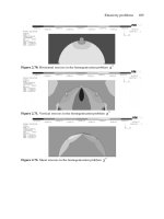
For the periodicity cell and its discretisation shown in Figure 2.128 elastic
properties of the glass fibre and the matrix are adopted as follows: the Young
moduli expected values E[e
1
] = 84 GPa, E[e
2
] = 4.0 GPa, while the deterministic
Poisson ratios are taken as equal to
ν

1
= 0.22 in fibre and
ν
2
= 0.34 – in the matrix.
Figure 2.128. Periodicity cell tested
Five different sets of Young moduli coefficients of variation are analysed
according to Table 2.21 − various values between 0.05 and 0.15 have been adopted
to verify the influence of the component data randomness on the respective
probabilistic moments of the homogenised elasticity tensor. The finite difference
numerical technique has been employed to determine the relevant derivatives with
respect to the input random variables adopted.
Table 2.21. The coefficient of variation of the input random variables
Test number
()
1
e
α
()
2
e
α
1 0.050 0.050
2 0.075 0.075
3 0.100 0.100
4 0.125 0.125
5 0.150 0.150
The cross-sectional fibre area equals to about a half of the total periodicity cell
area. The results in the form of expected values and coefficients of variation of the
homogenised tensor components obtained from four computational tests are shown

in Table 2.22 and compared against the corresponding values obtained by using the
MCS technique for the total number of random trials taken as 10
3
.
Table 2.22. Coefficients of variation for the effective elasticity tensor
Ω
1
Ω
2
Elasticity problems 145
Test
()
)(
)(
1111
ωα
eff
C
()
)(
)(
1122
ωα
eff
C
SFEM MCS SFEM MCS
1
0.0410 0.0516 0.7152 0.0517
2
0.0622 0.0777 0.1073 0.0777

3
0.0830 0.1037 0.1430 0.1037
4
0.1036 0.1297 0.1788 0.1297
5
0.1244 0.1557 0.2146 0.1557
It is seen that the results of the SFEM−based computations are slightly smaller
than those resulting from the Monte Carlo simulations in the case of
()
)(
)(
1111
ωα
eff
C
;
t
he opposite trend is observed for
()
)(
)(
1122
ωα
eff
C
. The differences between both
models are acceptable for very small input coefficients of variation and above the
value 0.1 (second order approach limitation) they enormously increase. It is also
observed that the coefficients from the MCS analysis are equal with each other,
while the SFEM returns different values for both effective tensor components. It

follows the fact that the first partial derivatives of both components with respect to
Young moduli of the fibre and matrix are different. These derivatives are included
in the SFEM equations for the second order moments and, in the same time, they
do not influence the MCS homogenisation model at all. Furthermore, a linear
dependence between the results obtained and the input coefficients of variation of
the components Young moduli is observed.
The main reason for numerical implementation of the SFEM equations for
modelling of the homogenisation problem is a decisive decrease in computation
time in comparison to that necessary by the MCS technique. It should be
mentioned that the Monte Carlo sampling time can be approximated as a product
of the following times:
(a) a single deterministic cell problem solution,
(b) the total number of homogenisation functions required (three functions
χ
(11)
, χ
(12)
and χ
(22)
in this plane strain analysis),
(c) the total number of random trials performed.
There are some time consuming procedures in the MCS programs such as
random numbers generation, post processing estimation procedure and the
subroutines for averaging the needed parameters within the RVE, which are not
included, however their times are negligible in comparison with the routines
pointed out before.
On the other hand, the time for Stochastic Finite Element Analysis can be
approximated by multiplication of the following procedure times: (a) the SFE
solution of the cell problem (with the same order of the cost considered as the
deterministic analysis) and the total number of necessary homogenisation

functions. Taking into account the remarks posed above, the difference in
computational time between MCS and SFEM approaches to the homogenisation
problem is of the order of about (n-1)τ provided that n is the total number of MCS
samples and τ stands for the time of a deterministic problem solution. Observing
this and considering negligible differences between the results of both these
146 Computational Mechanics of Composite Materials
methods for smaller random dispersion of input variables, the stochastic second
order and second moment computational analysis of composite materials should be
preferred in most engineering problems. The only disadvantage is the complexity
of the equations, which have to be implemented in the respective program as well
as the bounds dealing with randomness of input variables (the coefficients of
variation should be generally smaller than about 0.15).
2.3.4 Upper and Lower Bounds for Effective
Characteristics
Let us consider the coefficients of the following linear second order elliptic
problem [65]:
fuC =− ))((
εε
div ; Ω∈x
(2.230)
)()(
,,
2
1
εεε
ε
ijjiij
uu +=u ;
Ω∈
x

(2.231)
)()(
)(
pp
x
εεε
ψ
CC =
(2.232)
with boundary conditions
0=
ε
u ;
Ω∂∈
x
(2.233)
In the above equations )(,
εε
uu and f denote the displacement field, strain tensor
and vector of external loadings, respectively. As was presented in Sec. 2.3.3.2, the
effective (homogenised) tensor
0
C is such a tensor that replacing
ε
C and
0
C in
the above system gives
0
u as a solution, which is a weak limit of

ε
u with scale
parameter tends to 0. It should be mentioned that without any other assumptions on
Ω microgeometry the bounded set of effective properties is generated. Moreover, it
can be proved that there exist such tensors )inf(
ijkl
C and )sup(
ijkl
C that
)sup()inf(
0
ijklijklijkl
CCC ≤≤
(2.234)
It is well known that the theorem of minimum potential energy gives the upper
bounds of the effective tensor, whereas the minimum complementary energy
approximates the lower bounds. Thanks to the Eshelby formula the explicit
equations are as follows:
Elasticity problems 147
⎪
⎪
⎩
⎪
⎪
⎨
⎧
−
⎥
⎦
⎤

⎢
⎣
⎡
+=
−
⎥
⎦
⎤
⎢
⎣
⎡
+=
−
=
−
−
=
−
∑
∑
u
N
r
rur
u
N
r
rur
C
C

µµµµ
κκκκ
1
1
1
1
1
1
)(sup
)(sup
(2.235)
where
u
κ
,
u
µ
have the following form:
⎪
⎩
⎪
⎨
⎧
⎟
⎟
⎠
⎞
⎜
⎜
⎝

⎛
+
+=
=
−1
maxmaxmax
2
3
max
3
4
89
101
µκµ
µ
µκ
u
u
(2.236)
Further, lower bounds for the elasticity tensor are obtained as
⎪
⎪
⎩
⎪
⎪
⎨
⎧
−
⎥
⎦

⎤
⎢
⎣
⎡
+=
−
⎥
⎦
⎤
⎢
⎣
⎡
+=
−
=
−
−
=
−
∑
∑
l
N
r
rlr
l
N
r
rlr
C

C
µµµµ
κκκκ
1
1
1
1
1
1
)(inf
)(inf
(2.237)
where it holds that
⎪
⎩
⎪
⎨
⎧
⎟
⎟
⎠
⎞
⎜
⎜
⎝
⎛
+
+=
=
−1

minminmin
2
3
min
3
4
89
101
µκµ
µ
µκ
l
l
(2.328)
and n is a total number of composite constituents where nrc
r
≤≤1, denote their
volume fractions. It should be noted that
)21(3
υ
κ
−
=
e
(2.239)
)1(2
υ
µ
+
=

e
(2.240)
µκλ
3
2
−=
(2.241)
µδδδδλδδ
)(
jkiljlikklijijkl
C ++=
(2.242)
From the engineering point of view the most interesting is the effectiveness of
such a characterisation of
ijkl
C , which can be approximated as the difference
between upper and lower estimates and, on the other hand, sensitivity of the
148 Computational Mechanics of Composite Materials
effective tensor with respect to material characteristics of the constituents. The
Monte Carlo simulation technique has been used to compute probabilistic moments
of the effective elasticity tensor components for the periodic superconductor
analysed before. The superconducting cable consists of fibres made of a
superconductor placed around a thin walled pipe (tube) covered with a jacket and
insulating material. Experimental data describing elastic characteristics of the
composite constituents are collected in Table 2.23.
Table 2.23. Probabilistic elastic characteristics of the superconductor components
Material
E[e]
σ(e) E[
ν

] σ(
ν
)
316LN
205 GPa 8 GPa 0.265 0.010
Incoloy 908
‘annealed’
‘cold worked’
182 GPa
184 GPa
-
-
0.303
0.299
-
-
Titanium
126 GPa 12 GPa 0.311 0.012
Insulation
G10-CR
36 GPa - 0.21 -
Because of negligible differences in the elastic properties of Incoloy (between
the ‘annealed’ and ‘cold worked’ state) the ‘annealed’ state of the superconductor
is considered further. All the results obtained in the computational experiments
have been collected in Table 2.24 and Figures 2.129 2.137. Because of the fact
that the expected values appeared to be rather insensitive to the total number of
random trials in the Monte Carlo simulations, results of the relevant convergence
tests have been omitted in the tables and presented further in the figures. The
expected values considered have been collected in Table 2.24 for M=10,000
random trials.

Table 2.24. Effective elasticity tensor components and their expected values (in GPa)
Effective Analysis type
property Deterministic probabilistic
type
)(eff
JJJJ
C
)(eff
JKKJ
C
)(eff
JKJK
C
)(eff
JJJJ
C
)(eff
JKKJ
C
)(eff
JKJK
C
sup-VR
189.56 81.83 53.86 189.94 82.30 53.82
Sup
178.44 76.07 51.18 178.57 76.37 51.10
Inf
156.99 62.70 47.14 156.68 62.61 47.03
Inf-VR
137.93 51.86 43.03 137.54 51.71 42.92

Effective properties collected in this chapter (sup, inf in Table 2.24) have been
compared with the Voigt Reuss ones (sup-VR, inf-VR in Table 2.24). Considering
the results obtained, it should be noted that these first approximators are generally
more restrictive than the Voigt Reuss ones. Further, it can be observed that
deterministic values are, with acceptable accuracy, equal to the corresponding
expected values. Thus, for relatively small standard deviations of the input elastic
characteristics, the randomness in the effective characteristics can be neglected.
Elasticity problems 149
Finally, it can be noted that more restrictive bounds can be used to determine the
effective elasticity tensor in a more efficient way. Taking as a basis the arithmetic
average of the upper and lower bounds, the difference between these bounds is in
the range of 13% for
)(eff
JJJJ
C bound component, 19% for
)(eff
JKJK
C bound component
and 8% for
)(eff
JKKJ
C bound component.
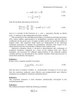
The following figures contain the results of the convergence analysis of the
coefficient of variation, asymmetry and concentration with respect to increasing
total number of Monte Carlo random trials. All these coefficients are presented for
)(eff
JJJJ
C bounds in Figures 2.129, 2.132 and 2.135, for
)(eff
JKJK

C bounds in Figures
2.130, 2.133 and 2.136 and for
)(eff
JKKJ
C in Figures 2.131, 2.134 and 2.137. On the
horizontal axes of these figures the total number of Monte Carlo random trials M is
marked, while the vertical is used for the coefficient of variation.
General observation here is that the
)(eff
JKJK
C bounds are the most sensitive with
respect to the randomness of input elastic characteristics. These coefficients for
)(eff
JKJK
C bounds appeared to be the greatest and then we obtain the coefficients for
)(eff
JJJJ
C and
)(eff
JKKJ
C , respectively. Next, it can be mentioned that the estimators of the
coefficients of variation show fast convergence to their limits. Efficient
approximation of final coefficients for various components of the tensor
)(eff
ijkl
C
bounds is obtained for M equal to about 2,500 random trials. Generally, it is
observed that the coefficients of variation of effective elasticity tensor fulfil the
inequalities detected in case of the expected values. The greatest coefficients are
obtained for Reuss bounds, next the upper and lower bounds proposed in this

chapter, and the smallest for the Voigt lower bounds.
4.70E-02
5.20E-02
5.70E-02
6.20E-02
6.70E-02
100 300 500 700 900 1500 2500 3500 4500 6000 8000 10000
sup - VR
sup
inf
inf - VR
Figure 2.129. The coefficients of variation of
)(eff
JJJJ
C
bounds
150 Computational Mechanics of Composite Materials
0.0650
0.0700
0.0750
0.0800
0.0850
0.0900
0.0950
0.1000
0.1050
100 300 500 700 900 1500 2500 3500 4500 6000 8000 10000
sup - VR
sup
inf

inf - VR
Figure 2.130. The coefficients of variation of
)(eff
JKJK
C
bounds
3.60E-02
3.70E-02
3.80E-02
3.90E-02
4.00E-02
4.10E-02
4.20E-02
4.30E-02
4.40E-02
4.50E-02
4.60E-02
100 300 500 700 900 1500 2500 3500 4500 6000 8000 1000
0
sup - VR
sup
inf
inf - VR
Figure 2.131. The coefficients of variation of
)(eff
JKKJ
C
bounds
-5.00E-07
-4.00E-07

-3.00E-07
-2.00E-07
-1.00E-07
0.00E+00
1.00E-07
2.00E-07
3.00E-07
4.00E-07
100 300 500 700 900 1500 2500 3500 4500 6000 8000 10000
sup - VR
sup
inf
inf - VR
Figure 2.132. The coefficients of asymmetry of
)(eff
JJJJ
C
bounds
Elasticity problems 151
-
4.00E-07
-
3.00E-07
-
2.00E-07
-
1.00E-07
0.00E+00
1.00E-07
2.00E-07

3.00E-07
4.00E-07
5.00E-07
6.00E-07
100 300 500 700 900 1500 2500 3500 4500 6000 8000 10000
sup - VR
sup
inf
inf - VR
Figure 2.133. The coefficients of asymmetry of bounds
-6.00E-07
-5.00E-07
-4.00E-07
-3.00E-07
-2.00E-07
-1.00E-07
0.00E+00
100 300 500 700 900 1500 2500 3500 4500 6000 8000 10000
sup - VR
sup
inf
inf - VR
Figure 2.134. The coefficients of asymmetry of
)(eff
JKKJ
C bounds
2.900
3.000
3.100
3.200

3.300
3.400
3.500
3.600
3.700
3.800
100 300 500 700 900 1500 2500 3500 4500 6000 8000 10000
sup - VR
sup
inf
inf - VR
152 Computational Mechanics of Composite Materials
Figure 2.135. The coefficients of concentration of
)(eff
JJJJ
C bounds
2.900
3.100
3.300
3.500
3.700
3.900
4.100
100 300 500 700 900 1500 2500 3500 4500 6000 8000 10000
sup - VR
sup
inf
inf - VR
Figure 2.136. The coefficients of concentration of
)(eff

JKJK
C bounds
2.800
3.000
3.200
3.400
3.600
3.800
4.000
4.200
100 300 500 700 900 1500 2500 3500 4500 6000 8000 10000
sup - VR
sup
inf
inf - VR
Figure 2.137. The coefficients of concentration of
)(eff
JKKJ
C bounds
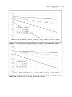
Observing the results presented in Figures 2.132 and 2.134 it can be observed
that all coefficients of asymmetry of
)(eff
ijkl
C verified tend to 0 with increasing total
number of random trials. Comparing
)(eff
JJJJ
C and
)(eff
JKJK

C against
)(eff
JKKJ
C bounds it can
be stated that the first two variables have minimum positive asymmetry, while the
last have a negative one. It should be mentioned that for such probabilistic
distributions with non zero coefficients of asymmetry, the expected value is not
equal to the most probable one.
Moreover, taking into account the convergence of coefficients of asymmetry it
is seen that they are generally more slowly convergent than coefficients of
variation estimators. M larger than 5,000 is required to compute these estimators
with satisfactory accuracy. Analogous to the coefficients of variation, the hierarchy
of the expected values of
)(eff
ijkl
C , which has been discussed above, is fulfilled.
Elasticity problems 153
Figures 2.135 2.137 present the coefficients of concentration for different
components of the effective elasticity tensor. The estimator convergence analysis
proves that M equal to almost 10,000 is needed to compute these coefficients
properly. The convergence of these estimators is more complex than the previous
ones, but generally their values are greater than 3, which is characteristic for the
Gaussian variables. Thus it can be stated that the
)(eff
ijkl
C
probabilistic distributions
obtained are more concentrated around their expected values than the Gaussian
variables, but this difference is no greater than a maximum of 15% for the
)(eff

JKJK
C
bounds.
Figures 2.138 2.140 illustrate the probability density functions of the upper
and lower bounds for
)(eff
JJJJ
C ,
)(eff
JKJK
C and
)(eff
JKKJ
C components of the effective
elasticity tensor. On the horizontal axes of these figures the values computed for
these components are marked, while on the vertical axes the relevant probability
density function (PDF) is given.
The PDFs for the tensor
)(eff
ijkl
C computed together with the additional
coefficients of asymmetry and concentration β, γ show that these functions have
distributions quite similar to the bell shaped Gaussian distribution curve. Thus, in
further analyses proposed in the conclusions, we assume that for the input random
variables being elastic characteristics (Young moduli and Poisson ratios) being
Gaussian uncorrelated random variables, the upper and lower bounds computed
having also a Gaussian distribution, which essentially simplifies further estimation
and related numerical analyses.
0
0.03

0.06
0.09
0.12
0.15
0.18
0.21
Ε−4σ Ε−3σ Ε−2σ Ε−σ Ε Ε+σ Ε+2σ Ε+3σ Ε+4σ
sup-VR
sup
inf
inf-VR
Figure 2.138. The probability densities of
)(eff
JJJJ
C bounds
154 Computational Mechanics of Composite Materials
0
0.03
0.06
0.09
0.12
0.15
0.18
0.21
Ε−4σ Ε−3σ Ε−2σ Ε−σ Ε Ε+σ Ε+2σ Ε+3σ Ε+4σ
sup-VR
sup
inf
inf-VR
Figure 2.139. The probability densities of

)(eff
JKJK
C bounds
0.00E+00
2.00E-02
4.00E-02
6.00E-02
8.00E-02
1.00E-01
1.20E-01
1.40E-01
1.60E-01
1.80E-01
2.00E-01
Ε−4σ Ε−3σ Ε−2σ Ε−σ Ε Ε+σ Ε+2σ Ε+3σ Ε+4σ
sup-VR
sup
inf
inf-VR
Figure 2.140. The probability densities of
)(eff
JKKJ
C bounds
The results of numerical tests performed lead us to the conclusion that the
probabilistic upper and lower bounds of the effective elasticity tensor may be very
efficient in the characterisation of superconducting composites with randomly
defined elastic characteristics because of negligible relative differences between
the upper and lower bounds. Considering the computational time cost they appear
to be much more useful in engineering practice than other FEM based direct
methods.

Computational experiments carried out prove that the coefficients of variation
of the bounds computed are in the range of the input random variables of the
problem. Considering further analyses of homogenised superconducting coils, this
fact confirms the need for the application of the SFEM in such computations,
which is important for essential time savings in comparison with the simulation
methods.
The probabilistic sensitivity of the effective elastic characteristics with respect
to the probabilistic material parameters should be verified computationally in
Elasticity problems 155
further analyses as an effect of regression test, for instance. Such an analysis
enables us to find out these parameters of composite constituent elastic
characteristics, which are the most influencing for global superconductor
behaviour.
The procedure for effective elastic properties approximation seems to be the
only method, which can be successfully applied to the homogenisation of
stochastic interface defects. Such an approach will make the elastic properties of
the interphases much more sensitive to the presence of structural defects than was
in case of the Probabilistic Averaging Method. Considering this, the bounds
presented should be implemented in numerical analysis of stochastic structural
defects into the artificial composite interphases.
2.3.5 Effective Constitutive Relations for the Steel
Reinforced Concrete Plates
The homogenisation method proposed for composite plates analysis is not
based on any mathematical model. However it seems to be very effective for high
contrast steel reinforced concrete plates [160]. The next main reason to apply this
model is that the composite plate need not be periodic in the applied approach,
which perfectly reflects the civil engineering needs. To get the effective
characterisation for the elasticity tensor, Eshelby theorem can be used since upper
and lower bounds for this tensor are determined. However it is proved by
comparison with collected experimental results, either lower and upper bounds are

very effective in computational modelling of a real plate. Both of them can be used
to calculate the zeroth, first and second order stiffness matrix and the resulting
probabilistic moments of displacements and stresses for the composite plate during
the SFEM analysis. It decisively simplifies the numerical analysis in comparison to
the traditional FEM modelling of such structures (where reinforcement
discretisation is complicated); more accurate results, especially in terms of thin
periodic plate vibration analysis, are shown in [155]. Finally, it should be
mentioned that the homogenised effective characteristics for composite shells can
be derived analogously, following considerations presented in [227,338].
Numerical test deals with the homogenisation of steel reinforced concrete
plates characterised by the data collected in Table 2.25; the coefficients of
variation randomized Young moduli are taken as 0.1 as in all previous
experiments. The concrete rectangular plate with horizontal dimensions 0.90 m x
0.90 m and thickness 0.045 m, supported at its corners and loaded by the vertical
concentrated force is examined and Table 2.26 contains the deterministic and
probabilistic homogenisation output. It can be observed that, as in previous
examples, the deterministic and expected values are close to each other,
respectively, and the resulting coefficients of variation are obtained as smaller or
equal to those taken for input random variables.
156 Computational Mechanics of Composite Materials
Table 2.25. Material data of the composite plate
Material properties Steel Concrete
Young modulus 200.0 GPa 28.6 GPa
Poisson ratio 0.30 0.15
Volume fraction 0.0367 0.9633
Yield stress 345.0 GPa 20.68 GPa
Table 2.26. Effective materials characteristics
Effective elasticity
tensor components
Deterministic Expected value Variation

()
[]
1111
inf CE
42.53 GPa 42.52 GPa 0.0985
()
[]
1111
sup
CE
44.84 GPa 44.84 GPa 0.0905
()
[]
1212
inf CE
13.13 GPa 13.12 GPa 0.0982
()
[]
1212
sup CE
13.88 GPa 13.88 GPa 0.0896
()
[]
1122
inf CE
16.27 GPa 16.28 GPa 0.0991
()
[]
1122
sup CE

17.09 GPa 17.09 GPa 0.0896
The most important observation is that the lower and upper bounds are almost
equal for any of the effective elasticity tensor components. Thus it does not matter
which of them are used in the approximation of the real composite structure.
Hence, the very complicated discretisation process of this particular concrete
structure type (ABAQUS) can be replaced with an analysis of the homogeneous
plate with elasticity tensor components calculated as proposed above. After
successful verification of other reinforced concrete plates with various
combinations of input parameters, such formulas for the effective elasticity tensor
could be incorporated in the finite element stiffness formation process to speed up
the FEM modelling procedures for these structures.
The variability analysis for expected values and the coefficients of variation of
the effective elasticity tensor is presented in Figures 2.141 and 2.142 as a function
of Young moduli expectations of the steel and concrete. It is seen that the Young
modulus of the concrete matrix is detected as a crucial parameter for both
probabilistic moments. It is due to the fact that the matrix is the dominating
component (in the volumetric context) while the equations for homogenised tensor
are rewritten as functions of the volume ratios of the composite components.
Considering the above, the behaviour of a real composite is compared against
the homogenised one, cf. Figure 2.143. It is seen that the central deflection
increments for both models are almost equal in the elastic range and, further, some
expressions for the nonlinear range should be proposed and verified.
Elasticity problems 157
Figure 2.141. Expected value of upper bound for the component C
1111
Figure 2.142. Coefficient of variation of upper bound for the component C
1111
A very broad discussion on theoretical and numerical modelling concepts in
reinforced concrete structures have been presented in [22] fracture analysis
contained in this study can be incorporated into the SFEM using the approach

described in [33]. Future analyses devoted to the application of homogenisation
technique in reinforced plates modelling should focus on incorporation of the
microcracks appearing in real matrices. It can be done using initial homogenisation
of the cracks into the matrix [92,266,321] to find equivalent homogeneous
medium; further homogenisation follows the above considerations.
Taking into account all the results of this test as well as the previous analyses
on the homogeneous plates with random parameters, the application of the
Stochastic Finite Element Method for the homogenised plate should approximate
the probabilistic moments of displacements [63] in linear elastic range for the real
plate very well. The expected values and variances of the effective elasticity tensor
can be obtained for this purpose by using symbolic MAPLE computations
analogous to those presented above.
158 Computational Mechanics of Composite Materials
Figure 2.143. Vertical displacements of the composite plate centre
2.4 Conclusions
The main advantage of the homogenisation approach proposed is that any
randomness in geometry or elasticity of the composite structures is replaced by a
single effective random variable of the elasticity tensor components characterising
such a structure. Hence, computational studies of engineering composites with
different random variables using a homogeneous one with deterministically
defined geometry and equivalent probability density function of the elastic
properties can be carried out. It is observed that using an analytical expression for
the homogenised elastic properties, the randomness in geometry for the periodicity
cell can be introduced and can result in random fluctuations of the effective
parameters only. Furthermore, even if the composite structure is not periodic, the
results of homogenisation method application are satisfactory, i.e. the probabilistic
response of the structure homogenised approximates very well the real composite
model; analytical solution in the correlative approach for random quasi periodic
structures can be found in [278].
The basic value of the proposed homogenisation method is that the equations

for the expected values and covariances of effective characteristics do not depend
on the PDF type of the input random fields. However, in case of greater values of
higher order probabilistic moments related to the first two as well as the lack of the
Elasticity problems 159
PDFs symmetry, a higher order version of the perturbation method is
recommended. It is important since the probability density function of the input
may not always be assumed properly, while in most experimental cases it is a
subject of the statistical approximation only. Application of a stochastic higher
order perturbation technique is relatively easy for closed form homogenisation
equations considering the symbolic differentiation approach. It should be
emphasised that, taking into account the capability of MAPLE links with
FORTRAN routines, the program can be used in further SFEM computations as an
intermediate procedure for symbolic homogenisation and sequential order
perturbation derivation.
It should be underlined that the method proposed can find its application in
stochastic reliability studies (SOSM approach) for various composite structures.
This homogenisation technique makes it possible to reduce significantly the total
number of degrees of freedom for such a structure, while the expected values and
covariances of displacements and stresses enable one to estimate the second order
second moment reliability (SORM) index or even third order reliability coefficients
(W-SOTM). In the same time, both probabilistic methodologies have
[171,175,180] and can find further applications in determination of effective heat
conductivity coefficients in various models [216,294] including fibre-reinforced
structures with some interfacial thermal resistance [303].
Due to the satisfactory accuracy of the homogenisation approach in modelling
of composite structures, the model worked out can be treated as the first step for
so called self homogenising finite elements, where the computer program
automatically homogenises the entire structure using original material composite
characteristics and finally calculates the displacements and stresses probabilistic
moments for an equivalent homogeneous medium. On the other hand, the

stochastic perturbation homogenisation procedure can be further modified for
elastoplastic composite structures using Transformation Field Analysis (TFA) or
Fast Fourier Transform (FFT) approaches. In the same time, the study of stochastic
elastodynamic effective behaviour is recommended since the still growing range of
composites has possible engineering applications.
2.5 Appendix
We prove, in the context of the composite model introduced in this chapter, that
u(x,y) being a solution of problem (2.121) is constant in the region Ω. For this
purpose, let us consider u(y) being a Ω periodic displacement function and the
solution of the following boundary value problem: