High Temperature Strain of Metals and Alloys Part 11 docx
Bạn đang xem bản rút gọn của tài liệu. Xem và tải ngay bản đầy đủ của tài liệu tại đây (455.64 KB, 15 trang )
148 8 Deformation of Some Refractory Metals
Fig. 8.5 The logarithm of strain rate versus stress in
molybdenum. The testing temperatures are B, 1973; C, 2173;
D, 2373; E, 2573; F, 2773 K (from 0.68 to 0.96 T
m
).
is presented in Fig. 8.9. The authors plot experimental data in log ˙ε − log σ
coordinates. Two segments of straight lines are observed at every test temper-
ature. At low stresses the creep rate is directly proportional to stress, so that
the factor in the power-law equation (1.1), n =1. At higher stresses factor n
increases abruptly to 8–9. The slope of the curves changes at critical stresses,
σ
cr
, 10, 20, and 70MPa at 1973, 1633 and 1033 K, respectively.
No creep strain with n =1was observed earlier. In Ref. [26] the authors
call it a high-temperature power-like creep. The primary stage covers nearly
80% of the strain to rupture. The polished surface of specimens exhibits slip
bands, thus, the slip of dislocations occurs.
The creep mechanism of molybdenum, which has a body-centered crys-
tal lattice, differs from the creep in metals that have a face-centered crystal
lattice. Unlike face-centered metals the minimum creep rate of molybde-
num depends weakly on temperature. The critical creep rates in the studied
temperature range (changes of flection coordinates) are from 2.2 × 10
−8
to
1.3×10
−8
s
−1
. The only visible effect is a shift of the function log ˙ε = f(log σ)
to higher stresses.
Molybdenum specimens have a random dislocation distribution after creep
in the range n =1. The ordered dislocation sub-boundaries cannot be formed
8.2 Alloys of Refractory Metals 149
Fig. 8.6 The logarithm of strain rate versus the inverse abso-
lute temperature for molybdenum. The applied stress,MPa,
is equal to: B, 9.81; C, 19.62; D, 29.43; E, 39.24; F, 49.05.
under n =1conditions. Only some grains close to the break stress between
segments n =1and n =8have sub-boundaries, obviously due to a local
overstress. At n =8one can observe well formed sub-boundaries. With in-
creasing stress the dislocation density in both sub-boundaries and subgrains
increases, and the structure eventually becomes cellular.
8.2
Alloys of Refractory Metals
A review of the creep behavior of refractory metal alloys has been published
[53].
A so called Larsom-Miller parameter, P , is widely used to estimate the creep
strength of alloys:
P = T [15 + log t
1%
]10
3
(8.1)
where T is temperature of the tests, t
1%
is the time of 1% deformation of a
specimen, 15 is an empirically determined value.
150 8 Deformation of Some Refractory Metals
Fig. 8.7 The measured activation energy of high-temperature strain
for molybdenum.
Fig. 8.8 The strain rate map for molybdenum with a grain
size of 100µm. Reprinted from Ref. [26].
8.2 Alloys of Refractory Metals 151
Fig. 8.9 The effect of stress on the
steady-state creep in molybdenum at
temperatures: 1, 1973; 2, 1633; 3, 1303 K.
Experimental data from Ref. [52].
One can see in Fig. 8.10 the typical creep behavior of the refractory metal
alloys. The corresponding nominal compositions of alloys are presented in
Table 8.3. Molybdenum-, niobium- and tantalum-based alloys have been de-
veloped, studied and utilized.
The creep properties of the refractory alloys are very sensitive to composi-
tion, structural features, and test environment. Small quantities of interstitial
atoms such as C, O and N may also have an important effect on the proper-
ties. Moreover, additional factors are possible, such as even the geographic
location from which the metal ore was obtained and technological features
during the production process.
Other factors affecting creep behavior include grain size, which can be
attributed to the annealing temperature (Fig. 8.11).
Many studies have been devoted to the search for potential strengtheners of
refractory metals. Incoherent or semi-coherent particles have been the most
commonly investigated. These precipitates are based on carbides. Hafnium
Tab. 8.3 Nominal composition of some refractory alloys.
Data from [53].
Curve Alloy Mo Ti Zr Nb Ta W Hf Re C
1 Mo-TZM bal. 1.0 0.75 – – – – – –
2 Nb-1Zr – – 1.0 bal. – – – – –
3 PWC-11 – – 1.0 bal – – – – 0.10
4 T-111 – – – – bal 8.0 2.0 – –
5 ASTAR-811C – – – – bal. 8.0 0.7 1.0 0.025
152 8 Deformation of Some Refractory Metals
Fig. 8.10 Applied stress to produce 1% creep strain in some
refractory alloys. Composition of alloys given in Table 8.3.
Reprinted from Ref. [53] with permission from Elsevier Science
Ltd.
carbide possesses the highest melting point. Tungsten–rhenium–hafnium
carbide alloys seem to be promising for operation at high temperatures.
Fig. 8.11 Effect of annealing temperature on applied stress
to produce 1% creep in ASTAR-81C alloy. 1, annealed at
1923 K; 2, annealed at 2273 K. Reprinted from Ref. [53].
8.2 Alloys of Refractory Metals 153
Fig. 8.12 Logarithm steady-stage creep rate versus the
logarithm stress for W–4Re–0.32HfC alloy. The testing
temperatures are B, 2200; C, 2300; D, 2400 K. Experimental
data from Ref. [54].
Park [54] compares some creep models with the experimental data on
the creep behavior of W–4Re–0.32HfC alloy. He obtained strain–time creep
curves of the tested alloy at 2200 K. Three regions of a creep curve are nor-
mally observed: primary, secondary and tertiary strain. The secondary creep
rate is assumed by the author to be expressed as ˙ε ∼ σ
n
[see Eq. (1.1)]. Three
straight parallel lines were obtained from this log ˙ε −log σ plot, Fig. 8.12, im-
plying that the secondary creep rate and the applied stress have a power-law
relationship. The value of n was obtained from the slope of each straight line,
and a least-squares analysis yielded n =5.2. Three creep models for second-
phase particle-strengthened alloys were applied to the creep behavior of the
alloy in this research. Park [54] studied the Ansell-Weertman, the Langeborg,
and the Roesler-Arzt models (the reader can find references in the quoted ar-
ticle). The conclusion was as follows: “The results showed that none of these
models predicted the creep behavior of the alloy”. Some models predicted the
secondary creep rate approximately five orders of magnitude different from
the value obtained experimentally.
However, the same experimental data satisfy another dependence, for ex-
ample, an exponential one. In Fig. 8.13 the same strain rates are plotted as
log ˙ε−σ. We also obtain straight lines which imply the dependence ˙ε ∼ exp σ.
We have noted (Chapter 1) that a functional dependence only makes it not
possible to conclude unequivocally about a physical mechanism of strain.
The orientation relationship between a matrix structure and a precipitate
structure have a dramatic effect on the creep deformation. The preferred
154 8 Deformation of Some Refractory Metals
Fig. 8.13 Logarithm steady-stage creep rate versus the stress
for W–4Re–0.32HfC alloy. The same experimental data as in
Fig. 8.12 from Ref. [54] are used.
orientation relationships between coherent and semi-coherent precipitates
and matrix may result in an improved resistance against slip of deforming
dislocations.
A niobium–titanium-based alloy has been investigated by Allamen et al.
[55]. The alloy under study contains 44Nb–35Ti–6Al–5Cr–8V–1W–0.5Mo–
0.3Hf. The microstructure of extruded and recrystallized material consists of
a solid solution and of particles of titanium carbide, TiC. The particle sizes
are between 200 and 500 nm. Creep curves were obtained at 977 K.
At relatively low stress, 103MPa, the slipping dislocations were attracted
to TiC particles. The attraction is energetically favored when the modulus
mismatch between the phases is decreased by diffusion. In contrast, a higher
density of dislocations is observed at the higher stress 172MPa, along with
bowed dislocations that are pinned by carbide particles.
The lattice periodicity in the [200]-type direction of the cubic body centered
matrix is about 0.33 nm. On the other hand, for the [220]-type direction of
the cubic face-centered precipitate, the lattice periodicity is about 0.32 nm.
The misfit is about 3%. This may explain why these two directions are nearly
parallel at the precipitate/matrix interface. A specific orientation relationship,
namely: [100](110) matrix parallel to [220](111) precipitates, was observed in
the specimens subjected to the highest stress level.
The development of superalloys for operation at temperatures up to 2073 K
continues. New classesofalloys attract investigators and engineers. Refractory
superalloys based on the platinum group metals have a cubic face centered
crystal lattice, high melting temperature, and a coherent two-phase structure.
8.3 Summary 155
A two-phase iridium-based refractory superalloy has been proposed re-
cently [56]. The alloy is strengthened by a coherent phase of L1
2
type. This
structure is similar to that of nickel-based superalloys. The authors investi-
gated the strength behavior and the structure of some binary iridium-based
alloys. The systems Ir–Nb and Ir–Zr are found to be the most promising alloys
for study at temperatures up to 1473 K.
The rupture life of Ir–Nb alloys was found to be increased dramatically
by the addition of nickel. The strengthening phase was determined to be
(Ni, Ir)
3
Nb. The steady-state creep rate at 1923 K for the Ir–15Nb–1Ni alloy
was 1.2 × 10
−8
s
−1
, about three orders of magnitude lower than that of the
binary Ir–17Nb alloy (10
−5
s
−1
).
This shows that the iridium-based alloys may possibly be regarded as ultra-
high temperature materials. However there is a lot of work ahead before new
alloys of this type can be used practically.
8.3
Summary
The physical properties of refractory metals are related to their high melting
points. They look very promising from the practical point of view. The most
refractory metals have, however, drawbacks such as poor low-temperature
fabricability and an extreme high-temperature oxidizability. When used they
need a protective atmosphere or a coating.
The minimum strain rate of niobium and molybdenum is dependent ex-
ponentially on the applied stress at high temperatures.
The mean value of the activation energy of the high-temperature strain for
niobium is found to be Q =(7.5 ± 0.6) × 10
−19
Jat.
−1
, for molybdenum
Q =(5.59 ± 0.35) ×10
−19
Jat.
−1
.
It follows from the experimental data that the rate-controlling mechanism
of strain for niobium is the slip of deforming dislocations with one-signed
jogs.
Molybdenum-, niobium- and tantalum-based alloys have been developed.
These alloys are able to operate at temperatures up to 1900 K. The creep
properties of the refractory alloys are very sensitive to composition, structural
features, and test environment. Other factors have yet to be studied in any
detail.
The alloys of the systems Ir–Nb and Ir–Zr are found to be the promising
for future study.
157
Supplements
Supplement 1: On Dislocations in the Crystal Lattice
The concept of dislocations is known to be important in the theory of strength
and plasticity [18, 20, 21]. Let us recall the main theses of the theory of dislo-
cations.
A crystal lattice is not ideal. The arrangement of atoms differs from a reg-
ular order. This is the immediate cause of the great discrepancy between
the theoretical strength of materials and the measured values. The practical
strength is about three orders less than the strength that would follow from
the concept of a regular atomic lattice. Any crystal lattice contains defects, i.e.
there are areas where the structure is irregular.
The point is that atoms on a slip plane do not displace simultaneously
under the effect of the applied stress. The atomic bonds do not break all at
the same time. The dislocation lines move along slip planes. A dislocation is
a one-dimensional defect. This means that the dislocation extent is compared
with the crystal size in only one dimension. In the two other dimensions
the dislocation has the extents of the interatomic order. The crystal lattice is
disturbed along the dislocation line. So the dislocation is the line defect in
the crystal lattice. It is like a stretched string.
There are two vectors, which determine the dislocation line at any point.
The dislocation line vector is denoted by
ξ. The Burgers vector is denoted by
b.
The unit vector
ξ is directed along the tangent to the dislocation line at every
point. It may be directed in a different way at different points of the same
dislocation line. The Burgers vector
b is related to the atomic displacements,
which the dislocation causes in the crystal lattice. The Burgers vector is the
same along a given dislocation, i.e. it does not change with the coordinates.
The magnitude of the Burgers vector is the interatomic distance b.Itisa
measure of deformation associated with the dislocation. The Burgers vector is
always directed along a close-packed crystallographic direction. This provides
High Temperature Strain of Metals and Alloys, Valim Levitin (Author)
Copyright
c
2006 WILEY-VCH Verlag GmbH & Co. KGaA, Weinheim
ISBN: 3-527-313389-9
158 Supplements
Fig. S1 Motion of the edge dislocation (⊥) in a crystal lattice
under the effect of shear stress.
the smallest value of b and, therefore, the lowest energy per unit length of
dislocation.
Dislocations move under the influence of external forces, which cause an
internal stress in a crystal slip plane. The force per unit length of dislocation,
F , exerted on the dislocation by the shear stress τ is F = bτ. The area swept
by the dislocation movement defines a slip plane, which always (by definition)
contains the vector
ξ.
In Fig. S1 the edge dislocation formation and its movement is shown.
Figure S1(a) demonstrates the generation of an edge dislocation by a shear
stress, dislocation is denoted as ⊥. In Fig.S1(b) movement of the dislocation
through the crystal occurs and an extra-plane appears above the slip plane.
The shift of the upper half of the crystal takes place after the dislocation
emerges from the crystal (Fig.S1(c)). The relative displacement of the two
crystal halves is normal to the dislocation. The Burgers vector of the edge
dislocation is perpendicular to the line vector, so the scalar product
(
b ·
ξ)=0
The edge dislocation can change its slip plane by means of a climb process.
In this connection completion of the extra-plane occurs. A diffusion flow of
vacancies or interstitial atoms is needed for the climb of the edge dislocation.
The climb is a slower process than the slip.
In Fig. S2 screw dislocation is shown, for screw dislocation vector
b is
parallel to vector
ξ:
(
b ·
ξ)=b
All dislocations have a character that is either pure edge, pure screw or a
combination of the two. In fact a dislocation is a boundary of a slip area. It
separates the area where the slip has occurred from the area where the slip
has not yet occurred. Dislocation lines may be arbitrarily curved. In Fig. S3
the arrangement of atoms in a mixed dislocation is shown. Atoms denoted
Supplement 1: On Dislocations in the Crystal Lattice 159
Fig. S2 A screw dislocation in the crystal lattice.
by large circles are situated over the diagram plane; those denoted by small
circles are situated under the diagram plane. We observe a transfer from the
pure screw to the pure edge dislocation.
In the general case one may consider the edge and screw components of
the mixed dislocation. In reality dislocation lines can have any shape, they can
form loops and networks and they can contain jogs, nodes, junctions, kinks.
The dislocation possesses an energy. The total energy per unit length is
the sum of the energy contained in the elastic field and the energy in the
dislocation core. The self-energy per unit length of dislocation, E
el
, depends
upon the magnitude of the Burgers vector and the shear modulus of the
material, µ,asE
el
≈ µb
2
.
The atoms nearest to the dislocation core are displaced most from their
equilibrium positions and therefore they have the highest energy. In order
to minimize this dislocation self-energy, the dislocation tries to be as short
as possible. That is, a dislocation prefers to minimize its length rather than
Fig. S3 A mixed dislocation
in a crystal lattice.
160 Supplements
meander through the crystal. This tendency to shorten itself, gives rise to the
concept of a dislocation line tension.
Inherent properties of dislocations are mobility and multiplication. Dislo-
cations move easily in their slip plane. The stress that a dislocation needs
to begin to move is of the order of 10
−4
µ, where µ is the shear modulus.
The velocity of dislocations is related to the applied stress and temperature.
Dislocations can multiply under the effect of external stress.
The quantity of dislocations in a crystal is measured by the dislocation
density: ρ = N/S, where N is the number of dislocations which intersect the
area S.
The strain of a crystal is given by equation ε = bρL, where L is the length
of the crystal.
A dislocation may dissociate into two so-called partial dislocations. A reason
for this dissociation is a gain in energy. Instead of a pure one dimensional
defect, the perfect dislocation, some kind of ribbon stretching through the
crystal is formed. This stacking fault ribbon may be constricted at some knots
or jogs. It is clear that a dislocation dissociated into two partials is able to slip
on the same plane as the perfect dislocation; the stacking fault just moves
along. It can also change its length.
In a face-centered crystal lattice the deformation occurs usually as the dis-
location slip in the crystal plane of type {111} in the < 110 > direction. The
Burgers vector is e.g.
b = a/2[110]. The dissociation happens according to
the reaction
a
2
[110] =
a
6
[121] +
a
6
[21
¯
1] (S.1)
Two Shockley dislocations are formed that can slip in the same plane {1
¯
11}.
The sum of Burgers vectors of two partial dislocations must be equal to the
Burgers vector of the complete dislocation:
b
1
+
b
2
=
b.
One must expect that there is an equilibrium distance d, which gives a
minimum energy for the split dislocation and the stacking fault. This equi-
librium distance depends mostly on the stacking fault energy γ. The smaller
γ the larger distance d between the partial dislocations; d is equal to four
interatomic distances in nickel and ten interatomic distances in copper. The
dissociation into partial dislocations hinders the climb of the dislocation into
parallel slip planes.
When a dislocation travels past two precipitates that are sufficiently far
apart, there is resistance set up to hinder the movement. More energy has to
be provided to move the dislocation past the barriers. Hence, the precipitates
strengthen the material via this mechanism. The evidence for the Orowan
mechanism lies in the residual dislocations that are often deposited around
the precipitates.
Supplement 2: On Screw Components in Sub-boundary Dislocation Networks 161
If a precipitate is sufficiently hard, it cannot be readily sheared by a disloca-
tion. In these cases, the dislocation will sometimes bow around the particle.
The applied stress exerts a force on the dislocation causing it to move. Points
along the dislocation are pinned by strong precipitates that are resistant to dis-
location penetration and shearing. The dislocation is able to bow out between
the precipitates, but the bowing process is resisted by the dislocation tension.
(Remember, the bowing of the dislocation creates more dislocation line and
increases the energy of the system). The dislocation is able to continue slip-
ping and a dislocation loop is left behind, circling the precipitate. This process
of circumventing a particle is called Orowan looping or dislocation bypass.
Supplement 2: On Screw Components in Sub-boundary Dislocation Networks
Prove the following theorem. Let us suppose that a low-angle dislocation sub-
boundary consists of two crossed but not perpendicular systems; within each
of the networks the dislocations are parallel and equidistant. The theorem
states that in these conditions dislocations at least of one system have a screw
component.
The notations are illustrated in Fig. S4. 1 and 2 are planes, in which are
located the systems under consideration.
ξ
1
and
ξ
2
are the unit vectors of
dislocation lines.
b
1
and
b
2
are Burgers vectors.
e
1
=(
b
1
×
ξ
1
)/|
b
1
|; e
2
=(
b
2
×
ξ
2
)/|
b
2
| are unit vectors of perpendiculars
to slip planes.
N
1
and
N
1
are inverse vectors, they lie in the boundary plane
and are perpendicular to dislocation lines. By definition
N
i
= N
i
(n ×
ξ
i
) (S.2)
where i =1, 2; N
i
=1/ηλ
i
. n =(
ξ
1
×
ξ
2
) is the unit vector of the perpendic-
ular to the sub-boundary plane.
It is known in the theory of low-angle sub-boundaries [18] that
N
1
=
b
2
−n(n ·
b
2
)
|
b
1
×
b
2
|
(S.3)
and
N
2
=
−
b
1
−n(n ·
b
1
)
|
b
1
×
b
2
|
(S.4)
Multiplying vectors
N
1
and
ξ
2
as scalars and taking into account Eq. (S.2)
we obtain
N
1
· [(n ×
ξ
1
) ·
ξ
2
]=
(
b
2
·
ξ
2
) − (n ·
ξ
2
)(n ·
b
2
)
|
b
1
×
b
2
|
(S.5)
162 Supplements
Fig. S4 The dislocation sub-boundary that
consists of two crossed systems of parallel
equidistant dislocations.
Similarly multiplying vectors
N
2
and
ξ
1
as scalars we obtain
N
2
· [(n ×
ξ
2
) ·
ξ
1
]=
(−
b
1
·
ξ
1
)+(n ·
ξ
1
)(n ·
b
1
)
|
b
1
×
b
2
|
(S.6)
However
(n ×
ξ
1
) ·
ξ
2
=(
ξ
1
×
ξ
2
) · n = n ·n =1; n ·
ξ
2
=0
and
(n ×
ξ
2
) ·
ξ
1
=(
ξ
2
×
ξ
1
) · n = −n ·n = −1; n ·
ξ
1
=0
Consequently we have
N
1
=
(
b
2
·
ξ
2
)
|
b
1
×
b
2
|
; N
2
=
(
b
1
·
ξ
1
)
|
b
1
×
b
2
|
(S.7)
The values of (
b ·
ξ) vary from 0 (for an edge dislocation) to ±b (for a screw
dislocation). According to the theorem condition it is impossible for N
1
=0
and N
2
=0at the same time. One can see from Eq. (S.7) that at least one
scalar multiplication is not equal to zero. This means that at least one system
contains a screw component.
Supplement 3: Composition of Superalloys 163
Supplement 3: Composition of Superalloys
In Table S1 the nominal contents of the main alloying elements are presented.
Typical third generation alloys include CMSX-4, EI867, ZhS26VI, TMS-75,
Rene N6, and the fourth generation include CMSX-10M, TMS-138.
Tab. S1 Nominal chemical composition (wt.%) of some nickel base superalloys.
Alloy Cr Al Ti Mo W Co Ta Nb Re Others Ref.
AM1 8.0 5.2 1.2 2.0 6.0 6.0 9.0 – – – 57
AM3 8.0 6.0 2.0 2.0 5.0 6.0 4.0 – – –
RWA 1480 10.0 5.0 1.5 4.0 – 5.0 12.0 – – –
Rene N4 9.0 3.7 4.2 2.0 6.0 8.0 4.0 0.5 – –
SRR99 8.0 5.5 2.2 – 10.0 5.0 3.0 – – –
AF56 12.0 3.4 4.2 2.0 4.0 8.0 5.0 – – –
RR2000 10.0 5.5 4.0 3.0 – – – – – 1.0V
C263 20.0 0.5 2.2 5.8 – 20.0 – – – 0.7Fe 58
CMSX-2 8.0 5.6 1.0 0.6 8.0 5.0 6.0 – – – 57
CMSX-3 7.9 5.6 1.0 0.5 8.0 4.6 6.0 – – 0.1Hf 43
CMSX-4 6.2 5.6 1.0 0.6 6.5 9.4 6.4 – 2.8 0.1Hf 46
CMSX-6 9.8 4.8 4.7 3.0 – 5.0 2.1 – – 0.1Hf 44
CMSX-10 2.0 4.8 0.2 0.4 5.0 3.0 8.0 – 6.0 0.03Hf 57
IN-X750 14.9 0.7 2.5 – – – 0.9 – 6,5Fe 39
EI437B 20.1 0.7 2.5 – – – – – – – Auth.
EI698 14.0 1.7 2.7 3.0 – – – 2.0 – –
EI867 9.5 4.5 – 9.8 5.3 5.1 – – – –
EP199 19.8 2.1 1.4 4.5 9.1 – – – – –
ZhS6UVI 9.4 5.6 2.5 1.5 10.1 9.6 – 1.1 – 0.5Hf
ZhS26VI 5.0 5.8 0.9 1.1 11.5 8.9 – 1.4 – 0.9V
Rene N5 7.0 6.2 – 2.0 5.0 8.0 7.0 – 3.0 0.2Hf 57
Rene N6 4.2 5.8 – 4.0 6.0 12.5 7.2 0.1 5.4 0.2Hf
CMSX-10M 2.0 5.8 0.2 0.4 5.4 1.8 8.2 0.1 6.5 – 34
MC544 4.0 6.0 0.5 1.0 5.0 – 5.0 – 4.0 0.1Hf
MC534 4.0 5.8 – 4.0 5.0 – 6.0 – 3.0 0.1Hf
Rene 80 14.5 3.8 3.8 – – 10.0 – – – 0.20C 59
MC2 8.0 5.0 1.5 2.0 8.0 5.0 6.0 – – – 57
SC180 5.0 5.2 1.0 2.0 5.0 10.0 9.0 – 3.0 0.1Hf
IN-100 12.4 5.0 4.3 3.2 – 18.5 – – – –
CM247LC 9.2 13.3 0.8 0.3 2.6 10.1 0.9 – – 0.5Hf 48
TMS-75 3.0 6.0 – 2.0 6.0 12.0 6.0 – 5.0 0.1Hf 49
TMS-138 3.0 6.0 – 3.0 6.0 6.0 6.0 – 5.0 0.1Hf 50
2.0Ru
LCAstroloy 15.1 4.0 3.5 5.2 – 17.0 – – – – 59
MAR-M200 9.0 5.0 2.0 – 12.5 10.0 – 1.0 – 0.05Zr
NASAIIB-7 8.9 3.4 0.7 2.0 7.6 9.1 10.1 – – 1.0Hf
Waspaloy 13.3 1.3 3.6 4.2 – 13.6 – – – –