Mechanics of Materials 1 Part 2 docx

53.8
Shearing Force and Bending Moment Diagrams
20
kN
60
kN
-2m
-
A
SF
(concentrated loads)
-56
7
1
Final
B
M.,
Fig.
3.14
1
I
I
I
H2=T
t
T2
53
Fig.
3.15.
S.F.,
B.M.

and
thrust
diagrams
for
system
of
inclined
loads.
54
Mechanics
of
Materials
$3.9
yield the values of the vertical reactions at the supports and hence the S.F. and
B.M.
diagrams
are obtained as described in the preceding sections. In addition, however, there must be a
horizontal constraint applied to the beam at one or both reactions to bring the horizontal
components of the applied loads into equilibrium. Thus there will be a horizontal force or
thrust diagram
for the beam which indicates the axial load carried by the beam at any point. If
the constraint
is
assumed to be applied at the right-hand end the thrust diagram
will
be
as
indicated.
3.9.
Graphical construction

of
S.F.
and
B.M.
diagrams
Consider the simply supported beam shown in Fig.
3.16
carrying three concentrated loads
of different values. The procedure to be followed for graphical construction of the
S.F.
and
B.M.
diagrams is as follows.
Y
X
Fig.
3.16.
Graphical construction
of
S.F.
and
B.M.
diagrams.
(a) Letter the spaces between the loads and reactions
A,
B,
C,
D
and
E.

Each force can then be
denoted by the letters of the spaces on either side of it.
(b) To one side of the beam diagram construct a force vector diagram for the applied loads,
i.e. set off a vertical distance
ab
to represent, in magnitude and direction, the force
W,
dividing spaces
A
and
B
to some scale,
bc
to represent
W,
and
cd
to represent
W,.
(c) Select any point
0,
known as
a
pole point,
and join
Oa,
Ob,
Oc
and
Od.

(d) Drop verticals from
all
loads and reactions.
(e) Select any point
X
on the vertical through reaction
R,
and from this point draw a line in
space
A
parallel to
Oa
to cut the vertical through
W,
in
a,.
In space
B
draw a line from
a,
parallel to
ob,
continue in space
C
parallel to
Oc,
and finally in space
D
parallel to
Od

to cut
the vertical through
Rz
in
Y:
$3.10
Shearing Force and Bending Moment Diagrams
55
(f) Join XY and through the pole point
0
draw a line parallel to XY to cut the force vector
diagram in
e.
The distance
ea
then represents the value of the reaction
R1
in magnitude
and direction and
de
represents
R2.
(g) Draw a horizontal line through
e
to cut the vertical projections from the loading points
and to act as the base line for the S.F. diagram. Horizontal lines from
a
in gap
A,
b

in gap
B,
c
in gap C, etc., produce the required S.F. diagram to the same scale as the original force
vector diagram.
(h) The diagram
Xa,b,c,Y
is the B.M. diagram for the beam, vertical distances from the
inclined base line XY giving the bending moment at any required point to a certain scale.
If the original beam diagram is drawn to a scale
1
cm
=
L
metres (say), the force vector
diagram scale is
1
cm
=
Wnewton, and, if the horizontal distance from the pole point
0
to the
vector diagram is
k
cm, then the scale of the B.M. diagram is
1
cm
=
kL
Wnewton metre

The above procedure applies for
beams carrying concentrated loads only, but an
approximate solution is obtained in
a
similar way for u.d.1.s. by considering the load divided
into a convenient number of concentrated loads acting at the centres
of
gravity of the
divisions chosen.
3.10.
S.F. and
B.M.
diagrams
for
beams carrying distributed loads
of
increasing value
For beams which carry distributed loads of varying intensity as in Fig.
3.18
a solution can
be obtained from eqn.
(3.3)
provided that the loading variation can be expressed in terms
of
the distance
x
along the beam span, i.e. as a function of
x.
Integrating once yields the shear force
Q

in terms of a constant of integration
A
since
dM
-=Q
dx
Integration again yields an expression for the B.M.
M
in terms of
A
and a second constant
of
integration B. Known conditions of B.M. or S.F., usually at the supports
or
ends of the beam,
yield the values of the constants and hence the required distributions of S.F. and
B.M.
A
typical example of this type
has
been evaluated on page
57.
3.11.
S.F. at points
of
application of concentrated loads
In the preceding sections it has been assumed that concentrated loads can
be
applied
precisely at a point

so
that S.F. diagrams are shown to change value suddenly from one value
to another, and sometimes one sign to another, at the loading points. It would appear from
the S.F. diagrams drawn previously, therefore, that two possible values of S.F. exist at any one
loading point and this is obviously not the case. In practice, loads can only be applied over
56
Mechanics
of
Materials
43.1
1
finite areas and the
S.F.
must change gradually from one value to another across these areas.
The vertical line portions of the
S.F.
diagrams are thus highly idealised versions of what
actually occurs in practice and should be replaced more accurately by lines slightly inclined to
the vertical. All sharp corners of the diagrams should also be rounded. Despite these minor
inaccuracies,
B.M.
and
S.F.
diagrams remain a highly convenient, powerful and useful
representation of beam loading conditions for design purposes.
Examples
Example
3.1
Draw the
S.F.

and
B.M.
diagrams for the beam loaded as shown in Fig.
3.17,
and determine
(a)
the position and magnitude of the maximum
B.M.,
and (b) the position of any point of
contraflexure.
L
I
S.F.
Diagram
/
+
\
Fig.
3.17.
Solution
Taking the moments about
A,
5RB=
(5
x
1)+(7
x
4)+(2
x
6)+(4

x
5)
x
2.5

5+28+12+50
=
19kN
5
R,
=
Shearing Force and Bending Moment
Diagrams
57
and since
R,+R,=
5+7+2+(4~5)= 34
RA=34-19=15kN
The
S.F.
diagram may now be constructed as described in
43.4
and is shown in Fig.
3.17.
Calculation
of
bending moments
B.M.
at
A

and
C
=
0
B.M.
at
B
B.M.
at
D
B.M.
at
E
=
-2x
1
=
-2kNm
=
-(2~2)+(19~1)-(4xlxi)= +13kNm
=
+(15~1)-(4xlx~)=
+13kNm
The maximum
B.M.
will be given by the point (or points) at which
dM/dx
(Le. the shear
force) is zero.
By

inspection
of
the S.F. diagram this occurs midway between
D
and
E,
i.e. at
1.5
m from
E.
B.M.
at this point
=
(2.5 x 15)
-
(5 x 1.5)
-
4
x 2.5 x
-
(
25)
=
+
17.5
kNm
There will also be local maxima at the other points where the
S.F.
diagram crosses its zero
axis, i.e. at point

B.
Owing to the presence of the concentrated loads (reactions) at these positions, however,
these will appear as discontinuities in the diagram; there will not
be
a smooth contour change.
The value
of
the
B.M.s
at these points should be checked since the position of maximum
stress in the beam depends upon the numerical maximum value of the
B.M.;
this does not
necessarily occur at the mathematical maximum obtained above.
The
B.M.
diagram
is
therefore as shown in Fig.
3.17.
Alternatively, the
B.M.
at any point
between
D
and
E
at
a
distance of

x
from
A
will be given by
42
2
M,,=
15~-5(~-1) = 1Ox+5-2x2
dM
dx
The maximum
B.M.
position
is
then given where
-
=
0.
x
=
2.5m
i.e.
1.5m from
E,
as found previously.
(b) Since the
B.M.
diagram only crosses the zero axis once there is only one point of
contraflexure, i.e. between
B

and
D.
Then,
B.M.
at distance
y
from
C
will be given by
My,
=
-
2y
+
19(y
-
1)
-
4(y
-
1)i
(y
-
1)
=
-2~~+19y-19-2~~+4~-2
=O
The point
of
contraflexure occurs where

B.M.
=
0,
i.e. where
My,
=
0,

0
=
-2yz+21y-21
58
Mechanics
of
Materials
i.e.
2y2-21y+21
=
0
Then
21
&
J(212
-
4
x
2
x
21)
=

1.12m
4
Y=
i.e. point of contraflexure occurs
0.12
m
to the left of
B.
Example
3.2
A
beam
ABC
is
9
m long and supported at B and
C,
6
m apart as shown in Fig.
3.18.
The
beam carries a triangular distribution of load over the portion
BC
together with an applied
counterclockwise couple of moment
80
kN m at Band a u.d.1. of
10
kN/m over
AB,

as shown.
Draw the S.F. and
B.M.
diagrams for the beam.
48
kN/m
I
I
-125
Fig.
3.18.
Solution
Taking moments about
B,
(R,
x
6)
+
(10
x
3
x
1.5)
+
80
=
(4
x
6
x

48)
x
4
x
6
6R,+45+80
=
288
R,
=
27.2
kN
and
R,+ R,
=
(10
x
3)+(4
x
6
x
48)
=
30+
144
=
174

R,
=

146.8
kN
Shearing Force and Bending Moment Diagrams
59
At any distance
x
from
C
between
C
and
B
the shear force is given by
S.F.,,
=
-
$WX
+
R,
w
48
x6
and by proportions
-
=-=a
i.e.

w
=
8x kN/m

S.F.,,
=
-
(R,-*
x
8~
x
X)
=
-R,+4x2
=
-27.2+4x2
The S.F. diagram
is
then as shown in Fig.
3.18.
Also
X
B.M.,,
=
-
(4
WX)-
+
R,x
3
4x3
=
27.2~
-_

3
For a maximum value,
i.e.,where
or
d
(B.M.)
-
S.F.
=
0
dX
4x2
=
27.2
x
=
2.61
m from
C
4
3
B.M.,,,
=
27.2(2.61)
-
-(2.61y
=
47.3kNm
B.M. at
A

and
C
=
0
B.M. immediately to left of
B
=
-
(10
x
3
x
1.5)
=
-45 kNm
At the point of application
of
the applied moment there will be a sudden change in B.M. of
80 kN
m.
(There will be no such discontinuity in the
S.F.
diagram; the effect of the moment
will merely be reflected in the values calculated for the reactions.)
The B.M. diagram is therefore as shown in Fig.
3.18.
Problems
3.1
(A). A
beam

AB, 1.2m long, is simply-supported at its ends
A
and Band carries two concentrated loads, one
of
10
kN at
C,
the other 15 kN at
D.
Point
C
is 0.4m from A, point
D
is 1 m from
A.
Draw the
S.F.
and
B.M.
diagrams
for the
beam
inserting principal values.
C9.17, -0.83, -15.83kN 3.67, 3.17kNm.l
3.2
(A).
The
beam
of question 3.1 carries an additional load
of

5
kN
upwards
at point
E,
0.6m from A. Draw the
S.F.
and
B.M.
diagrams for the modified loading. What is the maximum
B.M.?
C6.67, -3.33, 1.67, -13.33kN,2.67, 2,2.67kNm.]
3.3
(A). A
cantilever beam AB, 2.5 m long is rigidly built in at
A
and carries vertical concentrated loads of 8 kN at
[-8, -20kN; -11.2, -31.2kNm.l
B and 12 kN at
C,
1
m from A. Draw
S.F.
and
B.M.
diagrams for the beam inserting principal values.
60
Mechanics
of
Materials

3.4
(A).
A
beam
AB,
5
m
long, is simply-supported at the end
B
and at a point
C,
1
m
from A. It carries vertical
loads of
5
kN at
A
and 20kN at
D,
the centre of the span
BC.
Draw
S.F.
and
B.M.
diagrams for the beam inserting
principal values.
[-5,
11.25, -8.75kN;

-5,
17.5kNm.l
3.5
(A).
A
beam
AB,
3
m
long, is simply-supported at
A
and
E.
It carries a 16 kN concentrated load at
C,
1.2
m
from A, and a u.d.1. of
5
kN/m over the remainder of the beam. Draw the
S.F.
and
B.M.
diagrams and determine the
value of the maximum
B.M.
[12.3, -3.7, -12.7kN; 14.8kNm.]
3.6
(A). A
simply supported beam has a span of 4m and carries a uniformly distributed load of

60
kN/m together
with a central concentrated load of 40kN. Draw the
S.F.
and
B.M.
diagrams for the
beam
and hence determine the
maximum
B.M.
acting on the beam.
[S.F.
140, k20, -140kN;
B.M.0,
160,OkNm.l
3.7
(A).
A
2
m
long cantilever is built-in at the right-hand end and carries a load of
40
kN at the free end. In order
to restrict the deflection of the cantilever within reasonable limits an upward load of 10 kN is applied at mid-span.
Construct the
S.F.
and
B.M.
diagrams for the cantilever and hence determine the values of the reaction force and

moment at the support.
[30 kN, 70 kN m.]
3.8
(A).
A
beam 4.2m long overhangs each of two simple supports by 0.6m. The
beam
carries a uniformly
distributed load of 30 kN/m between supports together with concentrated loads of 20 kN and 30 kN at the two ends.
Sketch the
S.F.
and
B.M.
diagrams for the beam and hence determine the position of any points of contraflexure.
[S.F.
-20, +43, -47, +30kN
B.M.
-
12, 18.75,
-
18kNm; 0.313 and 2.553111 from 1.h. support.]
3.9
(A/B).
A
beam
ABCDE,
with
A
on the left, is 7
m

long and is simply supported at Band
E.
The lengths of the
various portions are AB
=
1.5
m,
BC
=
1.5
m,
CD
=
1
m
and
DE
=
3
m.
There is a uniformly distributed load of
15 kN/m between Band a point 2m to the right of
B
and concentrated loads
of
20 kN act at
A
and
D
with one of

50
kN at
C.
(a) Draw the
S.F.
diagrams and hence determine the position from
A
at which the
S.F.
is zero.
(b) Determine the value of the
B.M.
at this point.
(c) Sketch the
B.M.
diagram approximately to scale, quoting the principal values.
[3.32m;69.8kNm;O, -30,69.1, 68.1,OkNm.l
3.10
(A/B).
A
beam
ABCDE
is simply supported at
A
and
D.
It carries the following loading: a distributed load of
30 kN/m between
A
and

B
a concentrated load of 20 kN at
B;
a concentrated load of 20 kN at
C;
aconcentrated load
of 10 kN at
E;
a distributed load of
60
kN/m between
D
and
E.
Span
AB
=
1.5
m,
BC
=
CD
=
DE
=
1 m. Calculate
the value of the reactions at
A
and
D

and hence draw the
S.F.
and
B.M.
diagrams. What are the magnitude and
position of the maximum
B.M.
on the beam?
C41.1, 113.9kN; 28.15kNm; 1.37m from
A.]
3.11
(B).
A
beam, 12m long, is to be simply supported at 2m from each end and to carry a u.d.1. of 30kN/m
together with a 30 kN point load at the right-hand end.
For
ease
of
transportation the
beam
is to be jointed in two
places, one joint being situated
5
m
from the left-hand end. What load (to the nearest kN) must be applied to the left-
hand end to ensure that there is no
B.M.
at the joint (Le. the joint is to be
a
point ofcontraflexure)? What will then be

the best position on the beam for the other joint? Determine the position and magnitude of the maximum
B.M.
present on the beam.
[
114 kN, 1.6
m
from r.h. reaction; 4.7
m
from 1.h. reaction; 43.35 kN m.]
3.12
(B).
A
horizontal beam AB is 4
m
long and of constant flexural rigidity. It is rigidly built-in at the left-hand
end
A
and simply supported on a non-yielding support at the right-hand end
E.
The beam carries uniformly
distributed vertical loading of 18 kN/m over its whole length, together with a vertical downward load of lOkN at
2.5
m
from the end A. Sketch the
S.F.
and
B.M.
diagrams for the
beam,
indicating all main values.

[I. Struct. E.]
[S.F.
45, -10, -37.6kN;
B.M.
-18.6, +36.15kNm.]
3.13
(B).
A
beam ABC, 6
m
long, is simply-supported at the left-hand end
A
and at
B
1
m
from the right-hand end
C.
The beam is of weight 100N/metre run.
(a)
Determine the reactions at
A
and
8.
(b)
Construct
to
scales of 20
mm
=

1
m
and 20
mm
=
100 N, the shearing-force diagram for the beam, indicating
(c)
Determine the magnitude and position of the maximum bending moment.
(You
may, if you
so
wish, deduce
[C.G.] [240N, 360N, 288Nm, 2.4m from A.]
3.14
(B).
A
beam ABCD, 6
m
long, is simply-supported at the right-hand end
D
and at
a
point
B
lm from the left-
hand end
A.
It carries a vertical load of 10 kN at
A,
a second concentrated load of 20 kN at

C,
3
m
from
D,
and a
uniformly distributed load of 10 kN/m between
C
and
D.
Determine:
thereon the principal values.
the answers from the shearing force diagram without constructing a full
or
partial bending-moment diagram.)
(a)
the values of the reactions at
B
and
D,
(b)
the position and magnitude
of
the maximum bending moment.
[33 kN, 27 kN, 2.7
m
from
D,
36.45 k Nm.]
3.15

(B).
Abeam ABCDissimplysupportedat BandCwith
AB
=
CD
=
2m;BC
=
4m.Itcarriesapointloadof
60
kN at the free end A, a uniformly distributed load of
60
kN/m between Band C and an anticlockwise moment of
Shearing Force and Bending Moment Diagrams
61
80 kN
m
in the plane of the
beam
applied at the free end
D.
Sketch and dimension the
S.F.
and B.M. diagrams, and
determine the position and magnitude of the maximum bending moment.
[E.I.E.]
[S.F.
-60,
+170, -7OkN;B.M. -120, +120.1, +80kNm; 120.1kNmat 2.83m torightofB.1
3.16

(B). A
beam
ABCDE is 4.6m in length and loaded as shown in Fig. 3.19. Draw the S.F. and B.M. diagrams
for the
beam,
indicating all major values.
[I.E.I.] [S.F. 28.27, 7.06,
-
12.94, -30.94,
+
18,
0
B.M. 28.27, 7.06, 15.53,
-
10.8.1
E
Fig. 3.19
3.17
(B). A simply supported
beam
has a span
of
6m and carries a distributed load which varies in
a
linear
manner from 30 kN/m at one support to
90 kN/m at the other support. Locate the point
of
maximum bending
moment and calculate the value

of
this maximum. Sketch the
S.F.
and B.M. diagrams.
[U.L.] C3.25
m
from 1.h. end; 272 kN
m.]
3.18
(B). Obtain the relationship between the bending moment, shearing force, and intensity of loading
of
a
laterally loaded
beam.
A simply supported
beam
of span L carries a distributed load of intensity kx2/L2, where
x
is
measured from one support towards the other. Determine: (a) the location and magnitude of the greatest bending
moment, (b) the support reactions.
[U.
Birm.] C0.0394 kL2 at 0.63 of span; kL/12 and kL/4.]
3.19
(B). A
beam
ABC is continuous over two spans. It is built-in at
A,
supported on rollers at
B

and
C
and
contains a hinge at the centre
of
the span
AB.
The loading consists
of
a uniformly distributed load of total weight
20 kN
on
the 7
m
span
AB
and a concentrated load
of
30 kN at the centre of the 3 m span
BC.
Sketch the S.F. and
B.M. diagrams, indicating the magnitudes of all important values.
[I.E.I.]
[S.F.
5,
-15, 26.67, -3.33kN; B.M.4.38, -35, +5kNm.]
3.20
(B). A
log
of

wood 225
mm
square cross-section and
5
m
in
length is rendered impervious to water and floats
in a horizontal position in fresh water. It is loaded at the centre with a load just sufficient to sink it completely. Draw
S.F. and B.M. diagrams for thecondition when this load isapplied, stating their maximum values. Take thedensity
of
wood as 770 kg/m3 and of water as loo0 kg/m3. [S.F.
0,
+0.285,OkN; B.M. 0,0.356, OkNm.]
3.21
(B). A simply supported
beam
is 3
m
long and carries a vertical load of
5
kN at a point 1
m
from the left-hand
end. At a section
2
m
from
the left-hand end a clockwise couple of 3 kN m is exerted, the axis
of
the couple being

horizontal and perpendicular to the longtudinal axis of the
beam.
Draw to scale the B.M. and S.F. diagrams and
mark on them the principal dimensions. CI.Mech.E.1
[S.F.
2.33, -2.67 kN; B.M. 2.33, -0.34, +2.67 kNm.]
CHAPTER
4
BENDING
Summary
The simple theory
of
elastic bending states that
MaE
_-
_-
-
_-
IYR
where
M
is the applied bending moment
(B.M.)
at a transverse section,
I
is the second
moment of area of the beam cross-section about the neutral axis (N.A.),
0
is the stress at
distance

y
from the N.A. of the beam cross-section,
E
is the Young’s modulus of elasticity for
the beam material, and
R
is the radius of curvature of the N.A. at the section.
Certain assumptions and conditions must obtain before this theory can strictly be applied:
see page
64.
In some applications the following relationship is useful:
M
=
Zomax
where
Z
=
Z/y,,,and is termed the section modulus; amaxis then the stress at the maximum
distance from the N.A.
The most useful standard values of the second moment of area
I
for certain sections are as
follows (Fig.
4.1):
bd3
12
rectangle about axis through centroid
=
~
=

ZN,A,
bd3
3
nD4
64
rectangle about axis through side
=
__
=
I,,
circle about axis through centroid
=
-
=
ZN,A,
Fig.
4.1.
62
Bending
63
The
centroid
is the centre of area of the section through which the
N.A.,
or axis of zero stress,
is always found to pass.
In some cases it is convenient to determine the second moment of area about an axis other
than the
N.A.
and then to use the

parallel axis theorem.
IN,*.
=
I,+AhZ
For
composite beams
one material is replaced by an equivalent width of the other material
given by
where
EIE
is termed the
modular ratio.
The relationship between the stress in the material
and its equivalent area is then given by
E
E
0
=yo‘
For
skew loading
of
symmetrical sections
the stress at any point
(x,
y)
is given by
o=Iy+lX
Mxx
Myy
xx

YY
the angle of the
N.A.
being given by
Myy
Ixx
Mxx
I,,
tan6
=
f-
-
For
eccentric loading on one axis,
P Pey
(J=-+-
A-
I
the
N.A.
being positioned at a distance
I
Ae
y,=
f-
from the axis about which the eccentricity is measured.
For
eccentric loading on two axes,
P
Ph

Pk
a=-+-Xf-y
A
-I,,
Ixx
For
concrete or masonry rectangular or circular section columns,
the load must be retained
within the middle third or middle quarter areas respectively.
Introduction
If a piece of rubber, most conveniently of rectangular cross-section, is bent between one’s
fingers it is readily apparent that one surface of the rubber is stretched, i.e. put into tension,
and the opposite surface is compressed. The effect is clarified if, before bending, a regular set
of lines is drawn or scribed on each surface at a uniform spacing and perpendicular to the axis
64
Mechanics
of
Materials
$4.
I
of the rubber which is held between the fingers. After bending, the spacing between the set of
lines on one surface is clearly seen to increase and on the other surface to reduce. The thinner
the rubber, i.e. the closer the two marked faces, the smaller is the effect for the same applied
moment. The change in spacing of the lines on each surface is a measure of the strain and
hence the stress to which the surface is subjected and it is convenient to obtain a formula
relating the stress in the surface
to
the value of the
B.M.
applied and the amount

of
curvature
produced. In order for this to be achieved
it
is necessary to make certain simplifying
assumptions, and for this reason the theory introduced below is often termed the simple
theory
of
bending. The assumptions are as follows:
(1)
The beam is initially straight and unstressed.
(2)
The material of the beam is perfectly homogeneous and isotropic, i.e.
of
the same
density and elastic properties throughout.
(3)
The elastic limit is nowhere exceeded.
(4)
Young's modulus for the material is the same in tension and compression.
(5)
Plane cross-sections remain plane before and after bending.
(6)
Every cross-section of the beam is symmetrical about the plane of bending, i.e. about an
(7)
There is no resultant force perpendicular to any cross-section.
axis perpendicular to the N.A.
4.1.
Simple
bending

theory
If we now consider
a
beam initially unstressed and subjected
to
a constant
B.M.
along its
length, i.e. pure bending, as would be obtained by applying equal couples at each end, it will
bend
to
a radius
R
as shown in Fig.
4.2b.
As
a result of this bending the top fibres of the beam
will
be subjected to tension and the bottom to compression. It is reasonable to suppose,
therefore, that somewhere between the two there are points at which the stress
is
zero. The
locus of all such points is termed the
neutral axis.
The radius of curvature
R
is then measured
to this axis. For symmetrical sections the N.A. is the axis of symmetry, but whatever the section
the N.A. will always pass through the centre of area or centroid.
Fig.

4.2.
Beam
subjected to pure bending (a) before, and
(b)
after, the moment
M
has
been
applied.
Consider now two cross-sections
of
a beam,
HE
and
GF,
originally parallel (Fig. 423).
When the beam is bent (Fig. 4.2b) it is assumed that these sections remain plane; i.e.
HE
and
GF',
the final positions of the sections, are still straight lines. They will then subtend some
angle
0.
54.1
Bending
65
Consider now some fibre
AB
in the material, distance
y

from the
N.A.
When the beam is
bent this will stretch
to
A’B’.
A’B’
-
AB
-
-
extension
.
original length
AB
Strain in fibre
AB
=
But
AB
=
CD,
and, since the
N.A.
is unstressed,
CD
=
C‘D’.
A‘B‘
-

C‘D‘
(R
+
y)8
-
RB y
C’D‘
RB R

-
- -
strain
=
But
stress
strain
-
Young’s modulus
E
0
strain
=
-
E

Equating the two equations for strain,
or
Consider now a cross-section
of
the beam (Fig.

4.3).
From eqn.
(4.1)
the stress on a fibre at
E
R
distance
y
from the
N.A.
is
0=-y
Fig.
4.3.
Beam
cross-section.
If the strip is of area
6A
the force on the strip is
E
R
F
=
06A
=
-y6A
This has a moment about the
N.A.
of
66

Mechanics
of
Materials
$4.2
The total moment for the whole cross-section is therefore
E
R
=
-
Z
y26A
since
E
and
R
are assumed constant.
symbol
I.
The term
Cy26A
is called the
second moment
of
area
of the cross-section and given the
(4.2)
Combining eqns. (4.1) and (4.2) we have the bending theory equation
MaE
IYR
=-

-
(4.3)
From eqn. (4.2) it will be seen that if the beam is of uniform section, the material
of
the beam is
homogeneous and the applied moment is constant, the values of
I,
E
and
M
remain constant
and hence the radius of curvature of the bent beam will also be constant. Thus for pure
bending of uniform sections, beams will deflect into circular arcs and for this reason the term
circular bending
is often used. From eqn. (4.2) the radius of curvature to which any beam is
bent by an applied moment
M
is given by:
and is thus directly related to the value of the quantity
El.
Since the radius of curvature is a
direct indication of the degree of flexibility of the beam (the larger the value of
R,
the smaller
the deflection and the greater the rigidity) the quantity
El
is often termed the
jexural rigidity
or
flexural stiflness

of the beam. The relative stiffnesses of beam sections can then easily be
compared by their
El
values.
It should be observed here that the above proof has involved the assumption of pure
bending without any shear being present. From the work of the previous chapter it is clear
that in most practical beam loading cases shear and bending occur together at most points.
Inspection of the S.F. and
B.M. diagrams, however, shows that when the B.M. is a maximum
the
S.F.
is, in fact, always zero. It will be shown later that bending produces by far the greatest
magnitude of stress in all but a small minority of special loading cases
so
that beams designed
on the basis of the maximum
B.M.
using the simple bending theory are generally more than
adequate in strength at other points.
4.2.
Neutral
axis
As
stated above, it is clear that if, in bending, one surface of the beam is subjected to tension
and the opposite surface to compression there must be a region within the beamcross-section
at
which the stress changes sign, i.e. where the stress is zero, and this
is
termed the
neutral axis.

94.2
Bending
67
Further, eqn.
(4.3)
may be re-written in the form
M
I
a=-y
(4.4)
which shows that at any section the stress is directly proportional to
y,
the distance from the
N.A., i.e.
a
varies linearly with
y,
the maximum stress values occurring in the outside surface
of the beam where
y
is a maximum.
Consider again, therefore, the general beam cross-section
of
Fig.
4.3
in which the N.A. is
located at some arbitrary position. The force on the small element of area is
adA
acting
perpendicular to the cross-section, i.e. parallel to the beam axis. The total force parallel to the

beam axis is therefore
SadA.
Now one of the basic assumptions listed earlier states that when the beam is in equilibrium
there can be no resultant force across the section, i.e. the tensile force on one side of the N.A.
must exactly balance the compressive force on the other side.
adA
=
0
s

Substituting from eqn.
(4.1)
=
0
and hence
E
R
IydA
=
0
This integral is thefirst
moment
of
area
of the beam cross-section about the N.A. since
y
is
always measured from the N.A. Now the only first moment of area for the cross-section
which is zero is that about an axis through the centroid of the section since this is the basic
condition required of the centroid. It follows therefore that

rhe neutral axis must always pass
through the centroid.
It should be noted that this condition only applies with stresses maintained within the
elastic range and different conditions must be applied when stresses enter the plastic range
of
the materials concerned.
Typical stress distributions in bending are shown in Fig.
4.4.
It is evident that the material
near the N.A. is always subjected to relatively low stresses compared with the areas most
removed from the axis. In order to obtain the maximum resistance to bending it is advisable
therefore to use sections which have large areas as far away from the N.A. as possible.
For this
reason beams with
I-
or
T-sections find considerable favour in present engineering
applications, such as girders, where bending plays a large part. Such beams have large
moments of area about one axis and, provided that
it
is
ensured that bending takes place
about this axis, they will have a high resistance to bending stresses.
ut
IT.
Fig.
4.4.
Typical bending
stress
distributions.

68
Mechanics
of
Materials
$4.3
4.3.
Section
modulus
From eqn.
(4.4)
the maximum stress obtained in any cross-section is given by
M
I
omax=
-Ymax
(4.5)
For any given allowable stress the maximum moment which can be accepted by a particular
shape of cross-section is therefore
I
M=-
Ymax
For ready comparison of the strength of various beam cross-sections this is sometimes
written in the form
OmaX
M
=
Za,
(4.6)
where
Z(

=
I/ymax) is termed the
section
modulus.
The higher the value of
Z
for a particular
cross-section the higher the
B.M.
which it can withstand for a given maximum stress.
In applications such as cast-iron
or
reinforced concrete where the properties
of
the material
are vastly different in tension and compression two values of maximum allowable stress
apply. This is particularly important in the case of unsymmetrical sections such as T-sections
where the values of ymaxwi1l also
be
different on each side of the
N.A.
(Fig.
4.4)
and here two
values
of
section modulus are often quoted,
Z,
=
I/y, and

Z,
=Ily,
(4.7)
each being then used with the appropriate value of allowable stress.
Standard handbooks
t
are available which list section modulus values for a range of
girders, etc; to enable appropriate beams to be selected for known section modulus
requirements.
4.4.
Second moment
of
area
Consider the rectangular beam cross-section shown in Fig.
4.5
and an element of area
dA,
thickness
dy,
breadth
B
and distance
y
from the
N.A.
which by symmetry passes through the
Fig.
4.5.
t
Handbook

on
Structural Steelwork.
BCSA/CONSTRADO. London,
1971,
Supplement
1971,
2nd Supplement
1976
(in
accordance
with
BS449, ‘The
use
of
structural steel in building’).
Structural Steelwork Handbook for
Standard Metric Sections.
CONSTRADO. London,
1976
(in accordance with
BS4848,
‘Structural hollow sections’).
84.4
Bending
69
centre of the section. The
second moment
of
area
I

has been defined earlier as
I=
yZdA
Thus for the rectangular section the second moment of area about the
N.A.,
i.e. an axis
through the centre, is given by
I
012
Di2
-
DJ2
-D/2
=
B[$]yl,,
=
rz
BD3
Similarly, the second moment of area
of
the rectangular section about an axis through the
lower edge of the section would be found using the same procedure but with integral limits of
0
to
D.
These standard forms prove very convenient in the determination of
I
N.A.
values for built-up
sections which can

be
conveniently divided into rectangles. For
symmetrical sections
as, for
instance, the I-section shown in Fig.
4.6,
Fig.
4.6.
1N.A.
=
I
of dotted rectangle
-
I
of shaded portions
BD3
12
(4.10)
It will
be
found that any symmetrical section can
be
divided into convenient rectangles with
the
N.A.
running through each of their centroids and the above procedure can then be
employed to effect a rapid solution.
For
unsymmetrical sections
such as the T-section

of
Fig.
4.7
it
is
more convenient to divide
the section into rectangles with their
edges
in the
N.A.,
when the second type of standard form
may
be
applied.
IN.A
=
IABCD-
Ishaded
areas+
IEFGH
(abut
DC)
(abut
K)
(about
HC)
(each of these quantities may be written in the form
BD3/3).
70
Mechanics

of
Materials
$4.5
EF
U
Fig.
4.1.
As
an alternative procedure it is possible to determine the second moment of area of each
rectangle about an axis through its own centroid
(I,
=
8D3/12)
and to “shift” this value to
the equivalent value about the
N.A.
by
means of the
parallel
axis
theorem.
IN.A.
=
IG+
Ah2
where
A
is the area of the rectangle and
h
the distance

of
its centroid
G
from the
N.A.
Whilst
this is perhaps not
so
quick or convenient for sections built-up from rectangles, it is often the
only procedure available for sections of other shapes, e.g. rectangles containing circular holes.
(4.1
1)
4.5.
Bending
of
composite
or
flitcbed beams
(a)
A
composite beam is one which is constructed from a combination of materials. If such
a beam is hrmed by rigidly bolting together two timber joists and a reinforcing steel plate,
then it is termed a
Pitched beam.
Since the bending theory only holds good when a constant value of Young’s modulus
applies across a section it cannot be used directly to solve composite-beam problems where
two different materials, and therefore different values
of
E,
are present. The method of

solution in such a case is to replace one of the materials
by
an
equivalent section
of the other.
Steel
Wood
Equivalent
ore0
of
wood
repiocing
steel
Composite
section
Equivuient section
Fig.
4.8.
Bending
of
composite or flitched
beams:
original
beam
cross-section and
equivalent
of
uniform material
(wood)
properties.

Consider, therefore, the beam shown in Fig.
4.8
in which a steel plate is held centrally in an
appropriate recess between two blocks of wood. Here it is convenient to replace the steel by
an equivalent area of wood, retaining the same bending strength, i.e. the moment at any
section must
be
the same in the equivalent section as in the original
so
that the force at any
given
dy
in the equivalent beam must
be
equal to that at the strip it replaces.
54.6
Bending

since
atdy
=
a’t’dy
at
=
a’t’
&Et
=
&‘Et’
a
-=E

&
Again, for true similarity the strains must be equal,

E
=
E’
i.e.
E
E
t‘=-t
71
(4.12)
(4.13)
(4.14)
Thus
to replace the steel strip by an equivalent wooden strip the thickness must be multiplied
by the modular ratio
EIE.
The equivalent section is then one of the same material throughout and the simple bending
theory applies. The stress in the wooden part of the original beam is found directly and that in
the steel found from the value at the same point in the equivalent material as follows:
a
t’
a’
t
-

from eqn. (4.12)
-
and from eqn. (4.13)

aE
E
a‘
E
E
or
a= 6‘

-
(4.15)
i.e.
stress in steel
=
modular ratio
x
stress
in
equivalent
wood
The above procedure,
of
course, is not limited to the two materials treated above but
applies equally well for any material combination. The wood and steel flitched beam was
merely chosen as a convenient example.
4.6.
Reinforced concrete beams
-
simple tension reinforcement
Concrete has a high compressive strength but is very weak in tension. Therefore in
applications where tension is likely to result, e.g. bending, it is necessary to reinforce the

concrete by the insertion of steel rods. The section of Fig.’4.9a is thus a compound
beam
and
can
be
treated by reducing
it
to the equivalent concrete section, shown in Fig. 4.9b.
In calculations, the concrete is assumed to carry no tensile load; hence the gap below the
N.A. in Fig. 4.9b. The N.A. is then fixed since it must pass through the centroid of the area
assumed in this figure: i.e. moments of area about the N.A. must be zero.
Let
t
=
tensile stress in the steel,
c
=
compressive stress in the concrete,
A
=
total area of steel reinforcement,
rn
=
modular ratio,
Esteel/Econcrete,
other symbols representing the dimensions shown in Fig. 4.9.
72
Mechanics
of
Materiais

54.6
c
t/m
Total
A mA
Compressive force
in
concrete
Tensile force
in steel
(
d)
Fig.
4.9.
Bending of reinforced concrete
beams
with simple tension reinforcement.
(4.16)
h
2
bh
-
=
mA(d
-
h)
Then
which can
be
solved for

h.
The moment of resistance is then the moment of the couple in Fig. 4.9~ and
d.
Therefore
moment
of
resistance (based on compressive forces)
M=(bh)x
-
x
d
=-
d
area
2
(
:>
,,,(
:)
-~
.
-
average lever
stress arm
Similarly,
moment of resistance (based on tensile forces)
(4.17)
(4.18)
stress lever
arm

Both
t
and
c
are usually given as the maximum allowable values, which may or may not be
reached at the same time. Equations (4.17) and (4.18) must both
be
worked out, therefore, and
the lowest value taken, since the larger moment would give a stress greater than the allowed
maximum stress in the other material.
In design applications where the dimensions of reinforced concrete beams are required
which will carry a known
B.M.
the above equations generally contain too many unknowns,
$4.7
Bending
73
and certain simplifications are necessary. It is usual in these circumstances
to
assume a
balanced
section, i.e. one in which the maximum allowable stresses in the steel and concrete
occur simultaneously. There is then no wastage of materials, and for this reason the section is
also known as an
economic
or
critical
section.
For this type of section the N.A. is positioned by proportion of the stress distribution
(Fig. 4.9~).

Thus by similar triangles
c
tlm
h
(d-h)
=-
mc(d
-
h)
=
th
(4.19)
Thus
d
can be found in terms of
h,
and since the moment of resistance is known this
Also, with a balanced section,
relationship can be substituted in eqn. (4.17) to solve for the unknown depth
d.
moment of resistance (compressive)
=
moment of resistance (tensile)
bhc
2
__
=
At
(4.20)
By means of eqn. (4.20) the required total area of reinforcing steel

A
can thus be determined.
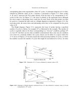
4.7. Skew loading (bending
of
symmetrical sections about axes
other than the axes
of
symmetry)
Consider the simple rectangular-section beam shown in Fig. 4.10 which is subjected to a
load inclined to the axes of symmetry. In such cases bending will take place about an inclined
axis, i.e. the N.A. will
be
inclined at some angle
6
to the
XX
axis and deflections will take place
perpendicular to the N.A.
Y
P
cos
a
I
‘\P
Y
Fig.
4.10.
Skew
loading
of

symmetrical section.
In such cases it is convenient to resolve the load
P,
and hence the applied moment, into its
components parallel with the axes of symmetry and to apply the simple bending theory to the
resulting bending about both axes. It is thus assumed that simple bending takes place
74
Mechanics
of
Materials
$4.8
simultaneously about both axes of symmetry, the total stress
at
any point
(x,
y)
being given
by
combining the results
of
the separate bending actions algebraically using the normal
conventions for the signs
of
the stress, i.e. tension-positive, compression-negative.
Thus
'
YY
The equation of the
N.A.
is obtained

by
setting eqn.
(4.21)
to
zero,
i.e.
(4.21)
(4.22)
4.8.
Combined bending and direct stress- eccentric loading
(a)
Eccentric loading on one
axis
There are numerous examples in engineering practice where tensile or compressive loads
on sections are not applied through the centroid of the section and which thus will introduce
not only tension or compression as the case may
be
but also considerable bending effects. In
concrete applications, for example, where the material is considerably weaker in tension than
in compression, any bending and hence tensile stresses which are introduced can often cause
severe problems. Consider, therefore, the beam shown in Fig.
4.1
1
where the load has been
applied at an eccentricity
e
from one axis of symmetry. The stress at any point is determined
by calculating the bending stress at the point on the basis of the simple bending theory and
combining this with the direct stress (load/area), taking due account of sign,
i.e.

where
M
=
applied moment
=
Pe
P
Pey

@E-+-
A-
Z
(4.23)
(4.24)
The positive sign between the two terms of the expression is used when both parts have the
same effect and the negative sign when one produces tension and the other compression.
Fig,
4.1
I.
Combined bending and direct stress -eccentric loading on one axis.
It should now be clear that any eccentric load can
be
treated as precisely equivalent to a
direct load acting through the centroid plus an applied moment about an axis through the
centroid equal to load
x
eccentricity. The distribution of stress across the section is then
given by Fig.
4.12.
54.8

Bending
75
Load
system
Jt=

+
M=pet-
e-

=
-
&

B$
N.A
-_
&
P
_________________
I
I
1-
Stress distribution/
Cornpressono-p Tension
Fig.
4.12.
Stress distributions under eccentric loading.
The
equation

of
the
N.A.
can
be
obtained by setting
t~
equal to zero in eqn. (4.24),
I
y=+-=
(4.25)
-Ae
yN
i.e.
Thus with the load eccentric to one axis the N.A. will be parallel to that axis and a distance
y,
from it. The larger the eccentricity
of
the load the nearer the N.A. will be to the axis
of
symmetry through the centroid for gwen values of
A
and
I.
(b)
Eccentric loading on two axes
It some cases the applied load will not be applied on either
of
the axes of symmetry
so

that
there will now be a direct stress effect plus simultaneous bending about both axes. Thus, for
the section shown in Fig. 4.13, with the load applied at
P
with eccentricities of
h
and
k,
the
total stress at any point
(x, y)
is given by
(4.26)
Fig.
4.13.
Eccentric loading on two axes showing possible position
of
neutral axis
SS
Again the
equation
of
the
N.A.
is obtained by equating eqn. (4.26) to zero, when
P Phx
Pky
-+ =o
A
-

I,,
I,,
76
Mechanics
of
Materials
$4.9
or
(4.27)
This equation is a linear equation in
x
and
y
so
that the N.A. is a straight line such as
SS
which
may or may not cut the section.
4.9.
“Middle-quarter” and “middle-third”
rules
It has been stated earlier that considerable problems may arise in the use of cast-iron or
concrete sections in applications in which eccentric loads are likely to occur since both
materials are notably weaker in tension than in compression. It is convenient, therefore, that
for rectangular and circular cross-sections, provided that the load is applied within certain
defined areas, no tension will be produced whatever the magnitude
of
the applied
compressive load. (Here we are solely interested in applications such as column and girder
design which are principally subjected to compression.)

Consider, therefore, the rectangular cross-section of Fig. 4.13. The stress at any point
(x,
y)
is given
by
eqn. (4.26) as
P Phx Pky
o=-+-+
-
A
-
I,,
I,,
Thus, with a compressive load applied, the most severe tension stresses are introduced when
the last two terms have their maximum value and are tensile in effect,
i.e.
For no tension to result in the section,
0
must be equated to zero,
1
6h 6k
o=
bd db2 bd2
or
bd
6
-=dh+bk
This is a linear expression in
h
and

k
producing the line
SS
in Fig. 4.13. If the load is now
applied in each of the other three quadrants the total limiting area within which
P
must
be
applied to produce zero tension in the section is obtained. This is the diamond area shown
shaded in Fig. 4.14 with diagonals of
b/3
and
d/3
and hence termed the
middle third.
For circular sections of diameter
d,
whatever the position of application of
P,
an axis of
symmetry will pass through this position
so
that the problem reduces to one of eccentricity
about a single axis of symmetry.
Now from eqn. (4.23)
P Pe
fJ-+-
A-I
§4.10
Bending

77
Fig. 4.14. Eccentric loading of rectangular sections-"middle third".
Therefore for zero tensile stress in the presence of an eccentric compressive load
~=~
A
4 d
=ex-x
2
64
nd4
1td2
d
e=8
Thus the limiting region for application of the load is the shaded circular area of diameter d/4
(shown in Fig. 4.15) which is termed the middle quarter.
Fig. 4.15. Eccentric loading of circular sections-"middle quarter".
4.10. Shear stresses owing to bending
It can be shown that any cross-section of a beam subjected to bending by transverse loads
experiences not only direct stresses as given by the bending theory but also shear stresses. The
magnitudes of these shear stresses at a particular section is always such that they sum up to
the total shear force Q at that section. A full treatment of the procedures used to determine the
distribution of the shear stresses is given. in Chapter 7.