Strength Analysis in Geomechanics Part 9 ppsx
Bạn đang xem bản rút gọn của tài liệu. Xem và tải ngay bản đầy đủ của tài liệu tại đây (480.27 KB, 20 trang )
5.3 Axisymmetric Problem 149
For the crack and punch we have two other border demands as f
(π)=0,
f
(0) = 1 and f
(π)=1,f
(0) = 0 respectively. It is interesting to notice that
once again the approximate solution gives at m = 1 the rigorous results.
Now we find f
,f
(see calculations in Appendix J) and according to (5.92) –
stresses σ
θ
, σ
r
, τ
rθ
, τ
e
., strain ε
θ
, displacement u
r
, integral J and factor K as
K
m+1
=(κ +1)πτ
2
l/2I(m)/f
(π)/
m
where I(m) is the same as in Sect. 5.2.1. Condition τ
e
= constant gives equation
forrinform
2r(2τ
e
)
m+1
GΩ(t)/τ
2
(κ +1)πl=F
m+1
/I(m)/f
(π)/
m
. (5.100)
Diagrams σ
θ
/σ
yi
, σ
r
/σ
yi
, τ
rθ
/σ
yi
are given in Fig. 3.11 by the same lines as
for m = 1 but with index 0. From the figure we can see that with the growth
of m the distribution of stresses changes very strongly. In the same manner
the problem of the punch horizontal movement can be considered. The curves
for the stresses can be received by reflection of the previous ones relatively to
axis θ = π/2.
5.3 Axisymmetric Problem
5.3.1 Generalization of Boussinesq’s Solution
As in Sect. 3.3.2 we suppose for incompressible material (ν =0.5) σ
χ
= σ
θ
=
τ
ρχ
= 0, and from the first static equation (2.77) as well as from rheological
law (1.29) at α = 0 we have for stress and strain following relations
σ
ρ
=f(χ)/ρ
2
, ε
ρ
=g(χ)Ω(t)ρ
−2m
(5.101)
whereg=f
m
. Since for this case in (2.79) ε
χ
= ε
θ
we find easily
u
χ
=U(ρ)sinχ, u
ρ
= ϕ(χ)+g(χ)Ω(t)ρ
1−2m
/(1 − 2m). (5.102)
Using condition ε
ρ
= −2ε
χ
we derive
0.5Ω(t)(3 − 2m)g(χ)ρ
1−2m
/(1 − 2m) + ϕ(χ)+U(ρ)cosχ =0. (5.103)
Putting u
ρ
,u
χ
from (5.102) into condition γ
ρχ
= 0 we determine
ϕ
(χ)+g
(χ)Ω(t)ρ
1−2m
/(1 − 2m) + ρ
2
(sin χ)∂(U(ρ)/ρ)/∂ρ. (5.104)
Excluding ϕ
(χ) from (5.103), (5.104) we obtain the expression in which
both parts must be equal to the same constant, say n, since each of them
depends only on one variable (neglecting t as a parameter) in form
Ω(t)g
(χ)/2sinχ = ρ
2m
dU(ρ)/dρ = −n
150 5 Ultimate State of Structures at Small Non-Linear Strains
P
Z
Fig. 5.17. Computation of constant n
with obvious solutions
f(χ)=Ω
−µ
(C + 2n cos χ)
µ
, U(ρ)=D− nρ
1−2m
/(1 − 2m). (5.105)
Since at χ = π/2 we have σ
ρ
= 0 we must put in the first (5.105) C = 0 and
constant n should be found from condition (Fig. 5.17)
P=−2
λ
0
σ
ρ
ρ
2
sin χ cos χdχ. (5.106)
Putting here σ
ρ
from (5.101) we find after calculations
σ
ρ
= −P(µ +2)cos
µ
χ/2π(1 − cos
µ+2
λ)ρ
2
. (5.107)
Taking in the second relation (5.105) D = 0 we get the displacement as
u
χ
= −Ω(t)(P(µ +2)/2π(1 − cos
2+µ
λ))
m
ρ
1−2m
(sin χ)/(1 − 2m). (5.108)
The most interesting case takes place at λ = π/2 when we receive from
expressions (5.107), (5.108)
σ
ρ
= −P(2 + µ)(cos
µ
χ)/2πρ
2
,
u
χ
= −Ω(t)(P(2 + µ)/2π)
m
ρ
1−2m
(sin χ)/(1 − 2m).
(5.109)
It is easy to notice that the highest value of σ
ρ
at ρ = constant is on the line
χ = 0. It is not difficult to find that there stress σ
ρ
at m = 1 is 1.5 times more
than at µ = 0. The biggest value of u
χ
is at χ = π/2 but its dependence on
m is more complex. However the second relation (5.109) allows to calculate
the displacements in some distance from the structure loaded by forces with
a resultant P.
5.3 Axisymmetric Problem 151
0 0.2 0.4
2
4
z/a
Fig. 5.18. Comparison of stress distribution
To appreciate a practical meaning of the results we compare for m = 1
the distribution of stress σ
z
on axis z for the concentrated force P = qa
2
and for the circular punch of radius a when we have from (5.109) and (3.122)
respectively
/σ
z
//q = 3(a/z)
2
/2π, σ
z
/q=1−(1 + (a/z)
2
)
−3/2
. (5.110)
From Fig. 5.18 where by solid and broken lines diagrams /σ
z
/(z) are shown
we can see that at z/a > 3 the simplest solution for concentrated force can be
used. Since at µ < 1 a distribution of stresses becomes more even we can
expect better coincidence of similar curves with the growth of a non-linearity.
It is interesting to notice that according to Figs. 5.18, 5.4 vertical stress in
axisymmetric problem is approximately twice less than in the plane one. This
explains higher load-bearing capacity of compact foundations.
5.3.2 Flow of Material within Cone
Common Equations
We solve this problem at the same suppositions as that in Sect. 4.3.3 From
(2.79) at u
χ
= 0 we compute
ε
ρ
= −2U/ρ
3
, ε
θ
= ε
χ
=U/ρ
3
,
γ
ρχ
≡ γ =dU/ρ
3
dχ, γ
m
=g/ρ
3
(5.111)
where U = U(χ)and
g(χ)=
9U
2
+U
2
.
Similar to (5.18) and (5.68) we use representations
ε
χ
= −g(cos 2ψ)/3ρ
3
, γ
ρχ
= g(sin 2ψ)/ρ
3
(5.112)
152 5 Ultimate State of Structures at Small Non-Linear Strains
putting which into the first law (2.82) we have equations
(g cos 2ψ)
+3gsin2ψ =0,
dg/gdχ = 2(dψ/dχ −3/2) tan 2ψ.
(5.113)
The latter gives boundary condition dψ/dχ = 3/2 at ψ = π/4. From expres-
sions for strains above we can also find
dln/U//dχ = −3 tan 2ψ, g(χ)=−3U/ cos 2ψ, (5.114)
From (5.17) and (5.112) we derive representations
τ
ρχ
= τ = ω(t)ρ
−3µ
g
µ
sin 2ψ,
σ
ρ
σ
χ
= ω(t)(C + ρ
−3µ
(K
+2
−1
x2g
µ
(cos 2ψ)/3))
(5.115)
where C is a constant and function K(θ) can be found from the first static
equation (2.77) as follows
3µK=(g
µ
sin 2ψ)
+cotχ(g
µ
sin 2ψ) + 4(1 − µ)g
µ
cos 2ψ. (5.116)
Putting (3.115) into (2.78) we derive
(g
µ
sin 2ψ)
+(g
µ
sin 2ψ)
cot χ +(9µ(1 − µ) − 1/ sin
2
χ)g
µ
sin 2ψ
+ 2(2 − 3µ)(g
µ
cos 2ψ)
=0.
(5.117)
Combining (5.113), (5.117) we have at Ψ according to (5.49) two differential
equations
Θ=dχ/dψ, (5.118)
(cot 2ψ)dΘ/dχ − 2(µ − 1+2µ/Ψ) + Θ((6µ
2
+3µ +4(1− µ)cos
2
2ψ)/Ψ
− cot χ cot 2ψ) − 3Θ
2
(3µ
2
− (µ + µ tan 2ψ cot χ +1/3sin
2
χ)cos
2
2ψ)/2Ψ = 0
(5.119)
the second of which should be solved at different Θ
o
= Θ. Then we integrate
(3.118) at border demand χ(0) = 0. The searched function must also satisfy
condition χ = λ at ψ = π/4. Now we receive from (5.113), (5.114), (2.65)
U(χ), g(χ)andτ
e
.
Putting stress σ
ρ
from (5.115) into integral static equation (4.105) we find
at −q
∗
= σ
ρ
(a, λ)=σ
χ
(a, λ) expression for max τ
e
as
max τ
e
=3µq
∗
maxg
µ
(χ)/((g
µ
(θ)sin2ψ)
χ=λ
− g
µ
(λ)cotλ −2J
3
/ sin
2
λ)
where
J
3
=
λ
0
g
µ
(θ)(sin 2ψ sin
2
χ +2cos2ψ sin 2χ)dχ.
Then the criteria max τ
e
= τ
u
and dγ
m
/dt →∞must be used as before. For
the latter we have
ε
∗
=1/α, Ω(t
∗
)=(αe2 max τ
e
)
−m
.
5.3 Axisymmetric Problem 153
Some Particular Cases
At µ = 0 we have the solution of Sect. 4.3.3.
If µ = 1 we compute from (5.113), (5.117) equation
(g sin 2ψ)
+(gsin2ψ)
cot χ +(6− 1/ sin
2
χ)g sin 2ψ =0
with obvious solution
gsin2ψ =2Dsin2χ (5.120)
where D is a constant. Then from (5.112)
gcos2ψ =3D(cos2χ −cos 2λ). (5.121)
From (5.120), (5.121) we receive
tan 2ψ = 2(sin 2χ)/3(cos 2χ −cos 2λ)
Diagrams ψ(χ) at different λ according to this relation are drawn in Fig. 5.19.
Similar to the general case we have ultimate condition as
max τ
e
=q
∗
x
1
2/3tanλ
(λ
>
<
33.7
◦
) (5.122)
At µ =2/3 we calculate from (5.117) equation
(g
2/3
sin 2ψ)
+(g
2/3
sin 2ψ)
cot χ +(2− 1/ sin
2
χ)g
2/3
sin 2ψ =0
with obvious solution solution
g
2/3
sin 2ψ =Hsinχ (5.123)
where H is a constant. Putting (5.123) into (5.113) we derive differential
equation of the first order
0
15
30
30 60
Fig. 5.19. Dependence ψ(χ)atµ =1
154 5 Ultimate State of Structures at Small Non-Linear Strains
0 60 120
2.3 3.051.280.58
1
15
30
4810
χ
o
ψ
o
Fig. 5.20. Diagrams ψ(χ)atµ =2/3 and different Θ
o
dχ/dψ = 2(2 + 3 cot
2
2ψ)/3(2 + cot χ cot 2ψ) (5.124)
that should be integrated at different Θ(0) = Θ
o
. Diagrams χ(ψ)atΘ
o
-values
in the curve’s middles and λ at their tops are given in Fig. 5.20.
Putting σ
ρ
from (5.113) into (4.105)we find C and from condition
dτ
e
/dχ = 0 with consideration of (5.124) – equality tan 2ψ = 3 tan χ which
gives to max τ
e
(it increases with a growth of χ) value
max τ
e
=q
∗
sin
2
λ
cos
2
λ +9sin
2
λ/(3 cos λ −cos
3
λ − 2 − 12J
4
).
Here as before −q
∗
= σ
ρ
(a, λ)=σ
χ
(a, λ)and
J
4
=
λ
0
(sin
2
χ cos χ)(tan 2ψ)
−1
dχ.
Diagrams J
4
(λ) and max τ
e
(λ) are shown in Figs. 5.21, 5.22 respectively. The
broken line in the latter picture refers to the case µ = 1 (computations for
µ =1/3 see in Appendix K-interrupted by points curve in the figure) and
pointed line refers to solution (4.106).
5.3.3 Cone Penetration and Load-Bearing Capacity
of Circular Pile
Here common relations (5.111). . . (5.119) are valid. We put stresses according
to (5.115) into integral static equations (4.107). to detail the constants and
according to (2.65) we compute max τ
e
at a = ρ as
5.3 Axisymmetric Problem 155
0
0.4
0.8
1.2
J
4
45 90 135
Fig. 5.21. Diagram J
4
(λ)forµ =2/3
0
1
2
30 60
Fig. 5.22. Diagram max τ
e
(λ)
max τ
e
=3µ(P/π − p
∗
(a + 1)
2
sin
2
λ)(maxg
µ
(χ))/a(a(2(g
µ
(χ)sin2ψ)
χ=λ
sin
2
λ
+g
µ
(λ)(1 + 3µ)sin2λ((1 + l/a)
2−3µ
− 1)/(2 − 3µ)
− l(g
µ
(λ)sin2λ +2J
5
)(2 + l/a)) (5.125)
where p
∗
is the strength of soil in a massif at compression and
J
5
=
λ
0
g
µ
(χ)((1 + 3µ)sin2ψ sin
2
χ +2cos2ψ sin 2χ)dχ.
At λ → π,a→∞we find for a circular pile
max τ
e
=(P/π − p
∗
b
2
)maxg
µ
(χ)/l(bg
µ
(λ)+J
5
(λ))(2 + l/a). (5.126)
In the same manner we consider the particular cases and consequently for
µ = 0 we receive from (5.117), equation (4.103) and hence the solution of
Sect. 4.3.4.
156 5 Ultimate State of Structures at Small Non-Linear Strains
At µ =1wehave
max τ
e
=4.5(P/π − p∗(a + 1)
2
sin
2
λ)x
1
2/3tanλ
/la(2(5 − 6sin
2
λ)/(1 + l/a)
− (2 + 3 sin
2
λ)(2 + l/a))
λ<146
◦
λ<146
◦
and for the pile the yielding (the first ultimate) load is
P
yi
= πb(2τ
yi
l+p
∗
b). (5.127)
We can see that this result has obvious structure and coincides with approxi-
mate relation (4.110) for ideal plasticity.
Similarly we compute for µ =2/3
max τ
e
=(P/π − p
∗
(a + 1)
2
sin
2
λ)
cos
2
λ +9sin
2
λ/6a(2a cos λ sin
2
λ ln(1 + l/a)
− l(2 + l/a)(1 − cos λ +2J
4
)).
Here J
4
is given in Sect. 5.3.2. For the circular pile this relation predicts big
values of ultimate load and so we can take in the safety side
P
u
= πb(p ∗ b+2τ
u
l). (5.128)
5.3.4 Fracture of Thick-Walled Elements Due to Damage
Stretched Plate with Hole
We consider plate of thickness h with axes r, θ, z (Fig. 5.23) and use the
Tresca-Saint-Venant hypotheses. Since here σ
θ
> σ
r
> σ
z
=0wehaveε
r
=0
and from (2.32) at α =0,σ
eq
=2τ
e
= σ
θ
ε ≡ ε
θ
= 3Ω(t)σ
θ
m
/4
σ
θ
=(4/3Ω)
µ
ε
µ
(5.129)
where ε =u/r and radial displacement u depends only on t.
Putting (5.129) into the static equation of this task
hσ
θ
=d(hrσ
r
)/dr, (5.130)
integrating it at h = constant as well as at boundary conditions σ
r
(a) = 0,
σ
r
(b) = p and excluding factor (4u/3Ω)
µ
we receive with the help of (5.129)
σ
θ
=p(1−µ)(b/r)
µ
/(1 − β
µ−1
) (5.131)
where β = b/a. Putting σ
θ
into (2.66) we find for the dangerous (internal)
surface
e
−αε
ε =3β(1 − µ)
m
Ω(t)p
m
(1 − β
µ−1
)
m
/4. (5.132)
Applying to (5.132) criterion dε/dt→∞we have
5.3 Axisymmetric Problem 157
a
b
r
u
p
Fig. 5.23. Stretched plate
ε
∗
=1/α, p
m
Ω(t
∗
) = 4(1 −β
µ−1
)
m
/3β(1 − µ)
m
αe. (5.133)
When the influence of time is negligible we compute from (5.133) at
Ω = constant critical load
p
∗
=(4/3)
µ
(1 − β
µ−1
)/(1 − µ)(αβΩe)
µ
. (5.134)
At small µ that value must be compared to ultimate load p
u
which follows
from (5.131) at µ → 0as
p
u
= σ
yi
(1 − 1/β)
where σ
yi
is a yielding point at an axial tension or compression and the small-
est value should be taken. At m near to unity we must compare p
∗
with
yielding load which follows from (5.131) at m = 1 in form:
p
yi
=(σ
yi
/β)lnβ
and the consequent choice should be made.
Sphere
For a sphere under internal q and external p pressures (Fig. 3.23) we denote
the radial displacement also as u and according to relations (2.80) we compute
ε
θ
=u/ρ, ε
ρ
= du/dρ and from the constant volume demand (2.81) we find
u=C/ρ
2
, ε
ρ
= −2C/ρ
3
, ε
θ
=C/ρ
3
=u/ρ (5.135)
where constant C is to be established from boundary conditions. Now from
(2.32) at α =0andσ
eq
= σ
θ
− σ
ρ
we deduce
158 5 Ultimate State of Structures at Small Non-Linear Strains
ε
θ
= Ω(t)(σ
θ
− σ
ρ
)
m
/2
or with consideration of (5.135)
σ
θ
− σ
ρ
= (2C/Ωρ
3
)
µ
. (5.136)
Putting (5.136) into static equation (2.80) we get after integration at border
demands σ
ρ
(b) = −p, σ
ρ
(a) = −q and exclusion of constants
σ
θ
− σ
ρ
= 3(q − p)µ(b/ρ)
3µ
/2(β
3µ
− 1). (5.137)
Now we use constitutive law (2.32) which for our structure is
e
−αε
ε =0.5Ω(t)(σ
θ
− σ
ρ
)
m
(5.138)
where ε = ε
θ
. Using here σ
θ
− σ
ρ
from (5.136) and criterion dε/dt→∞we
deduce
ε
∗
=1/α, (q −p)
m
Ω(t) = 2(2m/3)
m
(1 − β
−3µ
)
m
/αe. (5.139)
When the influence of time is not high critical difference of the pressures at
Ω = constant can be got
(q − p)
∗
=2
1+µ
m(1 − β
−3µ
)/3(αΩe)
µ
. (5.140)
At small µ this value should be compared with (q − p)
u
according to (4.97)
and the smaller one must be taken. Similar choice have to be fulfilled between
(q − p)
∗
and (q − p)
yi
given by (4.94) at µ near unity.
Cylinder
In an analogous way the fracture of a thick-walled tube can be studied. From
(2.32) at α =0,ε
x
=0,ε
θ
≡ ε and σ
eq
= σ
θ
− σ
r
we have
ε =(3/4)Ω(t)(σ
θ
− σ
r
)
m
(5.141)
and providing the procedure above for the disk and the sphere we find
/17, 27/
σ
θ
− σ
r
=2µ(q − p)(b/r)
2µ
/(β
2µ
− 1). (5.142)
Equation (2.32) for this structure is
e
−αε
ε = 3Ω(t)(σ
θ
− σ
r
)
m
/4. (5.143)
5.3 Axisymmetric Problem 159
Using here expression (5.142) at r = a and the criterion dε/dt →∞we derive
ε
∗
=1/α, (q − p)
m
Ω(t
∗
) = 4(m/2)
m
(1 − β
−2µ
)
m
/3αe. (5.144)
When influence of time is negligible we can find as before critical difference
of pressures as
(q − p)
∗
=(4/3)
µ
m(1 − β
−2µ
)/2(αΩe)
µ
and again for µ near to zero this value must be compared with (q − p)
u
according to (4.99) and smaller one have to be taken. The similar choice
should be made between (q − p)∗ and (q − p)
yi
from relation (4.98) at m
near unity.
From Fig. 5.24 where at α = 1, m = 1 and m = 2 by solid and broken lines
1, 2, 3 for plate, sphere and cylinder curves t
∗
(β) are represented respectively
we can see that the critical time for a tube is less than the consequent one for
the sphere and higher that of the plate.
Cone
We consider this task at the same suppositions as in Sect. 3.3.1 and Sect. 4.3.1.
Using the scheme above, relations for strains (3.117) and stresses (3.116) as
well as law (5.141) at σ
r
→ σ
χ
we find
σ
θ
− σ
χ
=(q−p) sin
µ
χ/J
6
sin
2µ
χ (5.145)
where
J
6
=
λ
ψ
(cos
1+µ
χ/ sin
2µ+1
χ)dχ. (5.146)
1
0
0.5
Ω
*
(q−p)
m
4
3
1
2
2
β
Fig. 5.24. Dependence of t
∗
on β and m
160 5 Ultimate State of Structures at Small Non-Linear Strains
The computations for m = 1 when J
6
=A/2 from Sect. 3.3.1 at λ = π/3,
ψ = π/6 show that integral J
6
can be easily calculated. For example at m = 2
and the shown meanings of λ, ψ its value is 0.9.
In order to appreciate the moment of fracture we put (5.145) into (5.143)
and use criterion dε/dt →∞when we have for a dangerous (internal) surface
ε
∗
=1/α, Ω(t
∗
)(q − p)
m
= 4(J
6
)
m
(sin
2
ψ)/3eα cos ψ. (5.147)
If the influence of time is negligible we derive from (5.147) at Ω = constant
(q − p)
∗
=(4/3)
µ
J
6
(sin
2
ψ/αeΩ cos ψ)
µ
. (5.148)
Once more for small µ this value must be compared with (q − p)
u
accord-
ing to (4.100) and smaller one should be taken. At µ near to unity (q −p)
∗
must be compared to (q − p)
yi
from Sect. 4.3.1 and similar choice should
be made.
Conclusion
The results of the solutions of this paragraph can be used for a prediction of
a failure not only of similar structures but also of the voids of different form
and dimension in soil massifs.
6
Ultimate State of Structures at Finite Strains
6.1 Use of Hoff’s Method
6.1.1 Tension of Elements Under Hydrostatic Pressure
This approach takes as the moment of a fracture time t
∞
when the structures’
dimensions become infinite. We consider as the first example a plate in tension
by stresses p under hydrostatic pressure q (Fig. 6.1). Since here σ
1
= σ
2
=p,
σ
3
= −q we have from (2.31)
dε/dt = 0.5B(p
o
)
m
(e
ε
+ κ
o
)
m
(6.1)
where ε = ε
1
, κ
o
=q/p
o
. and according to (1.42) p = p
o
e
ε
The integration of
(6.1) in limits 0 ≤ ε ≤∞,0≤ t ≤ t
∞
gives
B(p
o
)
m
t
∞
=2(ln(1+κ
o
)+(m−1)!
m−1
i=1
(−1)
i
(1 −i/(1 +κ
o
)
i
)/i!i(m −1 −i)!)/(κ
o
)
m
.
From Fig. 6.2 where for some κ
o
curves t
u
(µ) according to the latter expression
are given by broken lines we can see that t
u
≡ t
∞
diminishes with an increase
of hydrostatic component.
In a similar way the fracture time can be found for a bar in ten-
sion by stresses q under hydrostatic pressure p (Fig. 6.3). In this case /17/
σ
1
=q, σ
2
= σ
3
= −p and hence in (2.31)
S
1
= 2(p + q)/3, σ
eq
=p+q.
Comparing this data to the previous ones we can see that rate dε/dt in the
latter problem is twice of that for the plate. Hence t
∞
for the bar is one half
of that in the plate case.
162 6 Ultimate State of Structures at Finite Strains
q
qp
Fig. 6.1. Stretched plate under hydrostatic pressure
1.5
Bp
o
m
t
cr
1
0.5
0 0.25 0.5 0.75
2
1
0
2
1
0
µ
Fig. 6.2. Dependence of ultimate time t
cr
on κ
o
and µ
q
q
p
Fig. 6.3. Bar in tension under hydrostatic pressure
6.1.2 Fracture Time of Axisymmetrically Stretched Plate
In order to integrate differential equation (5.130) in the range of finite strains
we take according to the condition of Tresca-Saint-Venant in Sect. 5.3.4
r=r
o
+ u(t). We replace strains and displacements by their rates and rewrite
6.1 Use of Hoff’s Method 163
(5.130) with consideration of (5.129) at B instead of Ω (see (2.31)) and
dε/dt = dr/rdt as
d(r
o
h
o
σ
r
)/dr
o
=(4/3B)
µ
r
o
h
o
(r
o
+u)
−1−µ
(du/dt)
µ
. (6.2)
Integration of (6.2) at boundary conditions σ
r
(a
o
)=0, σ
r
(b
o
) = p gives
h
b
b
o
p=(4/3B)
µ
(du/dt)
µ
b
o
a
o
r
o
h
o
(r
o
)(r
o
+u)
−1−µ
dr
o
. (6.3)
Here h
b
=h
o
(b
o
). From (6.3) the fracture time can be found. Particularly at
h
o
= constant and h
o
=h
b
b
o
/r
o
we derive after transformations
B(b
o
p)
m
t
∞
=(4/3)
∞
0
(((b
o
+u)
1−µ
− (a
o
+u)
1−µ
)/(1 − µ)
+ u((b
o
+u)
−µ
− (a
o
+u)
−µ
)/µ)
m
du,
Bp
m
t
∞
=(4/3)m
m
∞
0
((a
o
+u)
−µ
− (b
o
+u)
−µ
)
m
du.
(6.4)
For any m integrals in (6.4) can be computed If e.g. m = 1 we have
respectively at β =b
o
/a
o
Bpt
∞
= 4(1 − 1/β)/3, Bpt
∞
=(4/3) ln β (6.5)
and from Fig. 6.4 where broken lines 0, 1 are drawn according to (6.5) we can
see that the curved profile has higher critical time. Broken 2 and interrupted
by points 1 lines refer to the cases m = 2, h
o
=h
b
b
o
/r
o
and h
o
= constant
when we derive from (6.4)
1
1
2
4
Bp
m
t
cr
2
2
2
1
0
1
1
β
Fig. 6.4. Dependence of ultimate time t
cr
on β and m for stretched plate
164 6 Ultimate State of Structures at Finite Strains
Bp
2
t
∞
= (16/3) ln((1 +
β)
4
/16β),
Bp
2
t
∞
= 16((3(1 + β
2
)/2+2β) − 2(1 + β)
β + 2(ln((1 +
β)/2)
+ β
2
ln((1 + 1/
β)/2))/3β
2
.
6.1.3 Thick-Walled Elements Under Internal
and External Pressures
We begin with a sphere and replace ε
θ
, u in (5.135) by their rates dε
θ
/dt,
V. Then we suppose in (5.136) Ω(t) = Bt. According to definition β =b/a
we have
dβ/dt = (db/dt −βda/dt)/a (6.6)
where
db/dt = V(b) = bdε
θ
(b)/dt, da/dt=V(a)=adε
θ
(a)/dt.
Using (5.136), (5.137) and (6.6) we derive after integration
B(q − p)
m
t
∞
= 2(2m/3)
m
β
0
1
((β
3µ
− 1)
m
/β(β
3
− 1))dβ. (6.7)
Here β
o
=b
o
/a
o
and critical time is equal to t
∞
. Diagram t
cr
(β
o
) according to
(6.7) at m = 1 is given in Fig. 6.5 by broken line 0. The curves for m = 2, m=3
go higher. For them
B(q − p)
2
t
∞
= 128(ln((β
o
3/2
+2)/2β
o
3/4
))/27,
B(q − p)
3
t
∞
= 16(ln β
o
+2
√
3 tan
−1
((1 − 1/β
o
)/
√
3)).
0
1
2
0
4
47
β
0
1
0
1.5
B(q−p)
m
t
cr
Fig. 6.5. Dependence of ultimate time t
cr
on β
o
and m for thick-walled elements
6.1 Use of Hoff’s Method 165
In a similar way the fracture of a cylinder can be considered. Using the
procedure above for the disk and the sphere we find
σ
θ
− σ
r
=2µ(q − p)(b/r)
2µ
/(β
2µ
− 1), (6.8)
B(q − p)
m
t
∞
=(4/3)(m/2)
m
β
o
1
((β
2
− 1)
m
/β(β
2
− 1))dβ. (6.9)
For m = 1 and m = 2 we compute respectively
B(q − p)t
∞
=(2/3) ln β
o
, B(q −p)
2
t
∞
=(4/3) ln((β
o
+1)
2
/4β
o
).
The consequent curves are drawn in Fig. 6.5 by broken lines 1, 2 and we can
see that for the tube t
∞
is less than that for the sphere.
For a cone we use the condition of its constant volume (4.101) and intro-
duce ratio
β =cosψ/ cos λ.
Then λ is function of β as
cos λ =((β
o
− 1)/(β − 1)) cos λ
o
and integral J
6
in (5.146) is also a function of β. Now we find
dβ/dt = (β −1)(tan λ)dλ/dt (6.10)
and since
ε(λ) = ln(sin λ/ sin λ
o
)
(Fig. 3.24) then
dλ/dt = tan λdε(λ)/dt
and from (5.141) with dε/dt, B instead of ε, Ω and (5.145) we derive
dε(λ)/dt = (3B/4)(q −p)
m
(cos λ)/(J
6
)
m
sin
2
λ. (6.11)
Putting dλ/dt together with (6.11) into (6.10), separating the variables and
integrating as before we have finally
B(q − p)
m
t
∞
=(4/3)(β
o
− 1) cos λ
o
1
β
o
(J
6
)
m
(β − 1)
−2
dβ. (6.12)
The integrals in (6.12) should be calculated as a rule approximately.
166 6 Ultimate State of Structures at Finite Strains
6.1.4 Final Notes
Although the method in this sub-chapter uses somewhat unrealistic supposi-
tion of an infinite elongation at the rupture, sometimes the fracture time is
near to test data. An analysis shows that the reason of it lays in the non-
linearity of equations linking the rate of strains with stresses. Because of that
the approach is widely used for the prediction of the failure moment of struc-
tures. For example in /17/ a row of elements are considered. Among them a
grating of two bars, thin-walled sphere and tube under internal pressure, a
long membrane loaded by hydrostatic pressure. Sometimes an initial plastic
deformation is also taken into account. The task of axisymmetric thin-walled
shells under the internal pressure is formulated. An attempt of consideration
of stress change on the base of creep hypotheses is also made. But the method
is mainly applied to a steady creep (see also Appendix L).
6.2 Mixed Fracture at Unsteady Creep
6.2.1 Tension Under Hydrostatic Pressure
For the bar in tension we use the notation of Fig. 6.3. According to relations
(1.42), (1.45) we can link conditional q
o
and true q stresses by expression
q=q
o
e
(1+α)ε
and from (2.32) we have
ε =0.5Ω(t)(q
o
)
m
(e
(1+α)ε
+k
o
)
m
. (6.13)
By criterion dε/dt →∞we find from (6.13)
ε
∗
= µ(κ
o
exp(−(1 + α)ε
∗
)+1)/(1 + α).
We can get critical time t
∗
by putting ε
∗
into (6.13). As we can see from
Fig. 6.6 the critical strains (at α = 0) increase with a growth of the hydrostatic
component.
In the same manner the failure of the plate in the axisymmetric tension
under hydrostatic pressure (Fig. 6.1) can be studied. As a result we have in
notation of Sect. 6.1.1
(p
o
)
m
Ω(t
∗
)=ε
∗
(exp(1 + α)ε
∗
+ κ
o
)
−m
and as we can see from Fig. 6.2 where for a steady creep (Ω = Bt) by solid
lines at the same κ
o
as the Hoff’s method diagrams t
∗
(µ) are constructed
critical time increases (similar to fracture time) with a fall of the hydrosta-
tic component. We can also notice that t
∗
< t
∞
and it can be shown (see
Appendix L) that with a growth of creep curves non-linearity the difference
between critical and fracture times increases. It can be explained first of all by
the circumstance that the method of infinite strain rate takes more realistic
condition of failure at finite strains than the Hoff’s approach.
6.2 Mixed Fracture at Unsteady Creep 167
0.5
1
ε
*
0.5
0
1
2
µ
0
Fig. 6.6. Dependence of ε
∗
on µ at different κ
o
for bar in tension under hydrostatic
pressure
6.2.2 Axisymmetric Tension of Variable Thickness Plate with Hole
General Case and that of Constant Thickness
Here /29/ we use the same suppositions as in Sect. 6.1.2 which bring equation
(2.33) to form
εe
−αε
=(3/4)Ω(t)(σ
θ
)
m
(6.14)
where ε = ε
θ
= ln(r/r
o
). Using the condition of a constant volume as
(r
o
+u)h=r
o
h
o
with u = u(t) we integrate differential equation (5.130) in initial variables as
follows
(3Ω/4)
µ
h
o
b
o
p=
b
0
a
0
h
o
(r
o
)(1 + u/r
o
)
−1−αµ
ln
µ
(1 + u/r
o
)dr
o
. (6.15)
If we seek the critical state with the help of a computer we can apply
criterion dε/dt →∞directly to expression (6.15). Calculated in this way
diagrams ε
b∗
(β) (here β =b
o
/a
o
), h
o
= constant, α =0andα =1are
represented in Fig. 6.7 by solid and broken lines 1. Critical time t
∗
for these
cases at Ω = Bt is given from (6.15) in Fig. 6.4 by solid curves 2 and 1.
Curved Profile
For the case h
o
=h
b
b
o
/r
o
, α = 0 we derive from (6.15) at du/dt →∞equality
b
0
a
0
(1 + u/r
o
)
−2
(µ ln
µ−1
(1 + u/r
o
) − ln
µ
(1 + u/r
o
))(r
o
)
−2
dr
o
=0
168 6 Ultimate State of Structures at Finite Strains
0.8
ε
*
0.4
0
14 7
3
2
4
2
1
0
β
Fig. 6.7. Dependence of ε
∗
on β for thick-walled structures
or after computing the integral
(1 + ξ
∗
/β)ln
µ
(1 + ξ
∗
)=(1+ξ
∗
)ln
µ
(1 + ξ
∗
/β)
where ξ =u/a
o
. This equation can be solved parametrically if we suppose
1+ξ
∗
/β =(1+ξ
∗
)
η
.
Here η is a parameter. We have from this equation
ξ
∗
= η
µ/(η−1)
− 1
and we can find other variables in form
β = ξ
∗
/((1 + ξ
∗
)
η
− 1), ε
b∗
= η ln(1 + ξ
∗
).
Curves ε
b∗
(β) are given by dotted lines 1 and 2 in Fig. 6.7 for m = 1 and
m = 2 respectively. When ξ
∗
isknownwecanfindt
∗
from (6.15) as
p
m
Ω(t
∗
)=(4/3)
β
1
(ξ
∗
+ ρ)
−1
ln
µ
(1 + ξ
∗
/ρ)dρ
m
where ρ =u/a
o
. Diagrams t
∗
(β) are drawn by dotted lines 1 and 2 in Fig. 6.4
for m = 1 and m = 2 respectively. We can see that in this case the curved
profile also gives higher critical time than that with h
o
= constant. This
indicates that an optimal profile can be searched.
Optimal Profile
We shall seek such a disk among ones with radial cross-sections as following
h
o
=a
o
(β − 1)
−1
((h
a
− βh
b
)b
o
/(r
o
)
2
+(β
2
h
b
− h
a
)/r
o
).