Power Quality Monitoring Analysis and Enhancement Part 9 docx
Bạn đang xem bản rút gọn của tài liệu. Xem và tải ngay bản đầy đủ của tài liệu tại đây (2.11 MB, 25 trang )
Single-Point Methods for Location of Distortion, Unbalance,
Voltage Fluctuation and Dips Sources in a Power System
187
to the substation A busbars. This results from significant differences in the lines lengths and
may occur in real systems.
Impedance under normal
operating conditions
Impedance under
disturbance conditions
No. of the
distance
protection
module
[Ω]
argument
[deg]
module
[Ω]
argument
[deg]
Z1 262.1 298.0 12.7 210.2
Z2 57.5 27.8 2.9 22.1
Z3 53.4 194.5 3.8 200.4
Table 2. Fault in the middle of line (F2)
Impedance under normal
operating conditions
Impedance under
disturbance conditions
No. of the
distance
protection
module
[Ω]
argument
[deg]
module
[Ω]
argument
[deg]
Z1 183.7 347.1 48.2 192.6
Z2 ∞
- ∞ -
Z3 183.5 167.4 48.2 12.9
Table 3. Fault at the origin of line 3 (F3) – line 2 disconnected
Impedance under normal
operating conditions
Impedance under
disturbance conditions
No. of the
distance
protection
module
[Ω]
argument
[deg]
module
[Ω]
argument
[deg]
Z1 262.1 298.0 13.8 48.5
Z2 57.5 27.8 37.0 246.9
Z3 53.4 194.5 22.0 214.7
Table 4. Fault at the origin of line 1 (F1)
Impedance under normal
operating conditions
Impedance under
disturbance conditions
No. of the
distance
protection
module
[Ω]
argument
[deg]
module
[Ω]
argument
[deg]
Z1 262.1 298.0 87 209.7
Z2 57.5 27.8 25.3 184.1
Z3 53.4 194.5 19.9 9.8
Table 5. Fault at the origin of line 3 (F3)
The method correctness depends to a large extent on the system configuration and this
dependence results from the method of operation of the distance protection.
3.8 Vector-space approach [28]
The testing of all these methods show that in cases of asymmetrical voltage dips, they are
rather ineffective. Furthermore, al the discussed methods, except the energy based one, require
computation of voltage and current phasors for the fundamental-frequency component.
Power Quality – Monitoring, Analysis and Enhancement
188
Because voltage dips are transient disturbance events, all phasor-based methods might produce
questionable results due to inherent averaging in the harmonic analysis of the input signals [28].
Type of
methods
Criterion Notes
>0 →
upstream
αβ,e
G−
αβ
u
αβαβ ,u
S i
Slope
()
u
tS t
,
(), ()
αβ αβ αβ
ui
<0 →
downstream
αβ,e
G+
αβ
u
αβαβ ,u
S i
Voltage-current method
where:
u
αβ
and i
αβ
-volta
g
e and current vectors defined in the ortho
g
onal coordinate
system αβ
ut()
αβ
- norm of the voltage vector u
αβ
()
uuii,,
α
β
α
β
- components of vector u
αβ
(i
αβ
) in the ortho
g
onal coordinate
system αβ
p
tuiui()
α
β
αα
ββ
=+ - instantaneous real power [1]
i
αβ
(t)=G
e,αβ
u
αβ
(t)
e
2
p
t
Gt
ut
,
()
()
()
αβ
αβ
αβ
=
()
e
SsignGt
,
()
αβ αβ
=
u
p
t
Si t
ut
,
()
()
()
αβ
αβ αβ
αβ
=
<0 →
upstream
Active
current
based
methods
If first peak of
()
e
SsignGt
,
()
αβ αβ
=
>0 →
downstream
Time response of
()
e
SsignGt
,
()
αβ αβ
= is
calculated for a few cycles before and
during voltage dips
>0 →
upstream
Impedance
based
methods
If
()
(
)
()
(
)
(
)
sign first peak t
sign first peak S i t
()
()
αβ
αβ αβ
Δ
Δ
u
<0 →
downstream
di
p
be
f
or di
p
ut ut ut() () ()
αβ αβ αβ
Δ= −
()
()
,,
,
() ()
()
uu
dip
u
be
f
ore di
p
Si t Si t
S i t
αβ αβ αβ αβ
αβ αβ
Δ= −
−
<0 →
upstream
Energy
based
method
If
t
0
wt p d() ( )
αβ αβ
ττ
Δ=Δ
>0 →
downstream
di
p
be
f
ore di
p
pt pt pt() () ()
αβ αβ αβ
Δ= −
Table 6. Voltage dip source detecting using vector space approach [28]
Single-Point Methods for Location of Distortion, Unbalance,
Voltage Fluctuation and Dips Sources in a Power System
189
In order to overcome these difficulties vector-space approach is proposed for voltage dip
detection. These methods are based on instantaneous voltage and current vectors and their
transformation into α,β,0 Clarke’s components. In this way other methods used for voltage
dip source detection like the system operating conditions trajectory during the dip (chapter
3.2), the active current based method (chapter 3.7.2), impedance based methods (chapter
3.7.1) and energy based method (chapter 3.4) can be presented in general form.
In Table 6 are presented the generalized methods using a vector space approach.
4. Voltage flictuations
Voltage fluctuations are a series of rms voltage changes or a variation of the voltage
envelope. Where only one dominant source of disturbance occurs its identification is usually
a simple task. In extensive networks or in the case of several loads interaction, the location
of a dominant disturbance source is a more complex process. Where large voltage
fluctuations occur in several branch lines it may happen that measurements of flicker
severity indices carried out at a power system node, do not indicate disturbing loads
downstream the measurement point. The reason is a mutual compensation of voltage
fluctuations from various sources.
(a)
(b)
Fig. 25. An example of changes in the flicker severity and the active and reactive power ―
phase L1 (diagram in (a))
Power Quality – Monitoring, Analysis and Enhancement
190
4.1 Criterion of voltage fluctuations during a fluctuating load operation and after
turning it off
The recorded quantities are: the flicker severity P
st
and changes in the reactive power Q (also
the active power P, if needed) at PCC. The measurements are carried out during the load
operation and, where technically possible, after it is turned off. An example records from a
steelwork during the arc furnace operation is shown in Fig. 25. Figure shows the results of
one week's measurement of the flicker severity P
st
, active power P and reactive power Q
(phase L1). The dependence of flicker severity values on changes in power, caused by the
arc furnace operation, is evident. During the periods the furnace is turned off the reactive
power at the measurement point is capacitive due to the presence of fixed capacitor banks.
In case several loads are analyzed the measurements have to be carried out during the
operation of each load separately.
4.2 Correlation of changes in the flicker severity P
st
and/or changes in the active and
reactive power
The method consists in the analysis of mutual correlation between changes in the reactive
power Q (and also the active power P, particularly for low-voltage networks) and the flicker
severity value P
st
. It allows define the dominant source of disturbance and assess the
influence of a change in the load power on the voltage fluctuation in the measurement point.
This method can also be applied for assessing the influence of disturbances in individual
branches of the network on the total P
st
at PCC.
(a) (b)
Fig. 26. An example of correlation characteristics of flicker severity P
st
and reactive power
changes
Fig. 26 shows correlation characteristics of flicker severity P
st
and reactive power changes.
Characteristic (a) exhibits a strong correlation; it means that a load supplied from the
monitored line is the dominant source of voltage fluctuation. In the case (b) the examined
load cannot be regarded to be the dominant source.
4.3 Examination of the U-I characteristic slope [23]
Consider two sources of flicker which cause voltage fluctuation at the measurement location
PCC: case 1 involves a flicker generating branch at point A and case 2 a similar at point B
(Fig. 1). As a result of this flicker caused in the system, the voltage measured at PCC will
fluctuate – the current at PCC will show different behaviour for these two cases, similar to
criterion used for voltage dip localization.
Single-Point Methods for Location of Distortion, Unbalance,
Voltage Fluctuation and Dips Sources in a Power System
191
For case 1, the measured current will be the load current at the lower voltage – the current
measured at PCC will decrease as the voltage decreases during the flicker occurrence, and
increase as the voltage increases (Fig. 27a).
For case 2, the measured current will be the sum of the load current and the flicker-caused
load current at the lower voltage – therefore, the current measured at PCC will increase as
the voltage decreases during the flicker occurrence, and decrease as the voltage increases
(Fig. 27b).
These observations are presented graphically in Fig. 27. Each event is characterized by
straight line, which represents the correlation between measured rms voltage and current. It
can be seen that the slopes of the lines are different for the two cases. A positive slope shows
that the flicker is from upstream and a negative slope shows that it is from downstream.
Although the idea was conceived for a one-source system, it has been found that it is also
valid for two-source system as in Fig. 15 [23].
0
0,05
0,1
0,15
0,2
0,25
0,3
0,35
0,4
0,45
0,5
0 0,05 0,1 0,15 0,2 0,25 0,3 0,35 0,4 0,45 0,5
Pst_L2_Brylewo
Pst_L2_GPZ15_sekcjaI
Volta
g
e U
PCC
(
rms
)
Current I
PCC
(rms)
Voltage U
PCC
(rms)
Current I
PCC
(rms)
a) b)
Fig. 27. Slope characteristics for the U-I correlations
4.4 Identification of interharmonic power direction [24]
The method utilises two common observations:
•
interharmonics cause flicker – the fundamental and an interharmonic component of a
voltage waveform are not in synchronous, therefore the voltage can be represented as
the one of with modulated magnitude, which causes flicker.
•
flicker cause interharmonics – voltage variations can be treated as amplitude
modulation of the voltage, therefore by means of Fourier analysis the voltage can be
decomposed on harmonic and interharmonic components.
Thus, the problem of locating flicker source can be solved by locating interharmonic source.
If the customer appears as a source of interharmonics i.e. the active interharmonic power is
negative, the customer is also a flicker source. If the customer appears as an interharmonic
load i.e. the active interharmonic power is positive, the customer is not a flicker source.
The method is applied as follows:
•
a power quality monitor is installed at the branch related to the suspected consumer,
and records voltage and current waveforms as flicker occurs.
•
Fourier based algorithm is used to investigate main interharmonics i.e. the components
that have the maximum magnitude.
•
for each of the interharmonic active power is calculated.
•
if the consumer produces interharmonic power, he can be identified as interharmonic
source and consequently the flicker source.
Power Quality – Monitoring, Analysis and Enhancement
192
The frequency of an interharmonic signal depends on operation of the customer's
equipment, so it is almost impossible that two devices produce the same interharmonics at
the same time. Consequently it is relatively easy to locate the source of interharmonics. This
method is fund not to be effective for random flicker source detection.
4.5 Examination of the "voltage fluctuation power"
A conception similar to the method of examining the direction of dominant interharmonics
active power flow is presented in [1,3,4]. Similarly to the definition of active power in the
time domain there could be introduced so called “flicker power”. Lets define supply voltage
and line current in PCC as sinusoidal waveforms with modulated amplitudes as follows
()()
11
() ()cos
PCC U
utUmt t
ω
=+
()()
11
() ()cos
PCC I I
it Imt t
ωϕ
=+ +
(43)
where u
PCC
(t), i
PCC
(t) are voltage and current waveforms respectively, U
1
, I
1
are magnitudes
of the fundamental components, m
I
(t), m
U
(t) are amplitude modulation function of current
and voltage respectively, ϕ
I
is phase shift of the current with respect to the voltage, ω
1
is the
angular frequency of the fundamental component.
The human sensitivity to flicker is a function of both modulating frequency and degree of
modulation. That means the frequency signals
()
U
mt and ()
I
mt must be filtered according
to how the human responds to flicker. This is achieved by using the sensitivity filter
described in the IEC 61000-4-15. The out signals
()
UF
mt and ()
IF
mt indicate how an average
human responds to flicker. By multiplying and integrating
()
UF
mt and ()
IF
mt a new
quantity “flicker power” FP is achieved:
0
1
() ()
T
UF IF
FP m t m t dt
T
=
(44)
where T is integration time. The flicker power provides two important pieces of information:
•
the sign of FP provides information whether flicker source is placed upstream or
downstream with respect to the monitoring point.
•
when several consumers are investigated, magnitude of FP provides information which
outgoing line contributes most to the actual flicker level.
Positive sign of flicker power means the same flow direction as the fundamental power
flow. It means that voltage modulation
()
U
mt is correlated with current modulation ()
I
mt
i.e. decreasing in supply voltage amplitude results in decreasing the load current.
Consequently the flicker source is placed upstream with respect to the measuring point.
Negative sign of flicker power means the opposite flow direction to the fundamental power
flow, and consequently the voltage modulation is negative correlated with current
modulation i.e. increasing the current load results in voltage drop. Therefore the flicker
source is placed downstream with respect to the measuring point meaning that the load is
responsible for voltage variation.
There could be noted, that the method is valid in a specific area of the load reactive power
variation.
The method gives correct results under inductive load (the current lags the voltage), and
limited capacitive power load (the current waveform leads the voltage waveform). There is
also possibility of misinterpretation when a load of constant power demand is considered.
Single-Point Methods for Location of Distortion, Unbalance,
Voltage Fluctuation and Dips Sources in a Power System
193
In such a case a voltage drop results in increased current flow. When the reaction is
considerable it could be misinterpreted as having the flicker source downstream. The
described situations, however, seldom arises in most practical situations.
5. Voltage asymmetry
A three-phase power system is called balanced or symmetrical if the three-phase voltages
and currents have the same amplitudes and their phases are shifted by 120° with respect to
each other. If either or both of these conditions are not fulfilled, the system is called
unbalanced or asymmetrical.
The generator terminal voltages provided to the power system are almost perfectly sinusoidal
in shape with equal magnitudes in the three phases and shifted by 120°. If the impedances of
the system components are linear and equal for three phases, and if all loads are three-phase
balanced, the voltages at any system bus will remain balanced. However, many loads are
single-phase and some large unbalanced loads may be connected at higher voltage levels (e.g.
traction systems, furnaces). The combined influence of such diverse loads, drawing different
currents in each phase, may give rise to the 3-phase supply voltage unbalance. The supply
voltage unbalance will then affect other customers connected to the same power network.
To quantify an unbalance in voltage or current of a three-phase system the symmetrical
components (Fortescue components) can be used. The three-phase system is thus
decomposed into a system of three symmetrical components: direct or positive-sequence,
inverse or negative-sequence and homopolar or zero-sequence, indicated by subscripts 1, 2,
0. These transformations are energy-invariant, so for any power quantity computed from
either the original or transformed values the same result is obtained. Thus, for active power
of a three-phase system we obtain the equation:
s
PP= (45)
where:
ABC AA A BB B BB C
cos cos cosPP P P UI UI UI
ϕϕϕ
=++= + +
and
s012 000111222
3( ) 3( cos cos cos )PPPP UI UI UI
ϕϕϕ
=++= + +
The subscripts A, B, C denote the different phases. It should be, however, noted that phase
active powers have positive direction (from a source to load). Active powers of the
symmetrical components
012
,,PPP have no physical meaning and their values depend on
the character of the system asymmetry. It can be demonstrated that active power of the direct
component has the same direction as the total system active power, but direction of active
power of the inverse component depends on the system asymmetry nature. Direction of the
inverse component may be used for identifying location of asymmetry source in the system.
~
~
~
A
B
C
U
U
1
RX
s
s
RX
n
n
I
measurement
Fig. 28. Circuit diagram for asymmetry source location identification
Power Quality – Monitoring, Analysis and Enhancement
194
Fig. 28 shows the circuit diagram for illustration the method, where equivalent parameters
U, R
s
, X
s
represent a power system side and R
n
, X
n
– load side.
Measured current
105
I
105
1
I
s
105
I
105
1
2
I
s
Measured voltage
100
50
U
1
50
25
1
U
1s
100
50
U
1
1
2
5025
U
1s
Source voltage
100
A
B
C
100
U
Active powers of
symmetrical
components
P
1
= 353.5
P
2
= 0
P
s
= 3(P
1s
+P
2s
) =
1060.5
P
1
= 352.2
P
2
= -29.0
P
s
= 3(P
1s
+P
2s
) = 969.6
Active power components
Load active
power
P
ABC
= 1060.5
P
ABC
= 969.6
Circuit
conditions
Symmetrical
Unbalanced load
side parameters
(balanced
system side
parameters
and phase
voltages)
Single-Point Methods for Location of Distortion, Unbalance,
Voltage Fluctuation and Dips Sources in a Power System
195
105
I
105
1
2
I
s
105
I
105
1
2
I
s
100
50
U
1
1
2
5025
0
U
1s
100
50
U
1
1
2
5025
0
U
1s
100
U
100
50
U
P
1
= 397.8
P
2
= 29.0
P
s
= 3(P
1s
+P
2s
) =1280.4
P
1
= 245.5
P
2
= 9.8
P
s
= 3(P
1s
+P
2s
) =765.9
P
ABC
= 1280.4
P
ABC
= 765.9
Unbalanced
system side
parameters
(balanced load
side
parameters and
phase voltages)
Unbalanced
system phase
voltages
(balanced
system side
parameters and
load side
parameters)
Table 7. Comparative asymmetry analysis in the point of measurement
Power Quality – Monitoring, Analysis and Enhancement
196
In order to examine the method of asymmetry source locating in the analysed diagram the
following parameters are taken (in per unit values): U = 100; R
s
= R
n
= R = 3.536 and X
s
=
X
n
= X = 3.536. Thus, for symmetrical conditions we obtain: I = 10 and U
1
= 50.
The following sources of asymmetry in the circuit in Fig. 25 are considered:
-
unbalanced load side parameters: R
nA
= 0.1R, R
nB
= R, R
nC
= 2R,
X
nA
= 0.1X, X
nB
= X, X
nC
= 2X
-
unbalanced system side parameters: R
sA
= 0.1R, R
sB
= R, R
sC
= 2R,
X
sA
= 0.1X, X
sB
= X, X
sC
= 2X
-
unbalanced system phase voltages:
0
0
j
A
UUe= ,
0
120
0,5
j
B
UUe
−
= ,
0
120j
C
UUe=
Results of the calculation are shown in Table 7. As can be seen, the positive sign of the
inverse component active power indicates the system side as the source of asymmetry at the
point of measurement (irrespective to voltage or impedance asymmetry), the negative sign
of the inverse component active power indicates the load side as the source of asymmetry.
6. Conclusion
In many cases, the quantitative determination of the supplier's and customer's share in the
total disturbance level at the point of common coupling (PCC) is also required. Seeking non-
expensive, reliable and unambiguous methods for locating disturbances and assessing their
emission levels in power system, not employing complex instrumentation, is one of the
main research areas which require the prompt solution. As a result, such research has
become an important topic recently.
7. References
[1] Akagi H., Kanazawa Y., Nabae A.: Generalized theory of instantaneous reactive power in
three-phase circuit, Proceedings of the International Power Electronics Conference,
Tokyo, Japan, 1983, 1375-1386.
[2] Axelberg P.G.V., Bolen M., Gu L.: A measurement method for determining the direction
of propagation of flicker and for tracing a flicker source, International Conference
CIRED’2005, Turin (Italy), June 2005.
[3] Axelberg P.G.V., Bollen M.,: An algorithm for determining the direction to a flicker
source, IEEE Trans. on Power Delivery, 21, 2, 755-760, 2006.
[4] Axelberg P.G.V., Bollen M., Gu L.: Trace of flicker sources using the quantity of flicker
power, IEEE Tran. On Power Delivery, 23, 1, 465-471, 2008.
[5] D’Antona G., Muscas C., Sulis S.: Harmonic source estimation: a new approach for the
localization of nonlinear loads, 978- 1-4244- 1 770-4/08, 2008 IEEE.
[6] Bollen M.H.J.: Understanding power quality problems – voltage sags and interruptions.
IEEE Press Series on Power Engineering 2000.
[7] Chang G. W., Chen C. I, Teng Y. F.: An application of radial basis function neural
network for harmonics detection, 978-1-4244-1770-4/08,2008 IEEE.
[8] Chen C., Liu X, Koval D.,, Xu W., Tayjasanant T.: Critical impedance method - a new
detecting harmonic sources method in distribution systems, IEEE Transactions on
Power Delivery, 19, 1, January 2004.
[9] Cristaldi L., Ferrero A.: Harmonic power flow analysis for the measurement of the
electric power quality, IEEE Tran. Instrum. Meas, 44, 6,1995, pp. 683-685.
Single-Point Methods for Location of Distortion, Unbalance,
Voltage Fluctuation and Dips Sources in a Power System
197
[10] Dán A.M.: Identification of flicker sources, 8
th
ICHQP ’98, Athens, Greece, Oct. 14-16,
1998.
[11] De Jaeger E.: Measurement of flicker transfer coefficient from HV to MV and LV
systems. UIEPQ-9630.
[12] De Jaeger E.: Measurement and evaluation of the flicker emission level from a particular
fluctuating load, CIGRE/CIRED Joint Task Force C4.109, Oct. 2007.
[13] De Jaeger E.: Disturbances emission levels assessment techniques (CIGRE/CIRED Joint
Working Group C4-109).
[14] Emanuel A. E.: On the assessment of harmonic pollution, IEEE Trans. on Power Delivery,
10, 3, 1995.
[15] Guide to quality of electrical supply for industrial installations. Part 5: Flicker, UIEPQ 1999.
[16] Hamzah N., Mohamed A., Hussain A.: A new approach to locate the voltage sag source
using real current component, Electric Power Systems Research, 2004, vol. 72, pp. 113-23.
[17] IEEE guide for protective relay applications to transmission lines, IEEE Std. C37.113,
1999.
[18] IEEE Power Engineering Society, Distribution System Analysis Subcommitee, IEEE 37
Node Test Feeder
[19] Khosrayi A., Melendez J., Colomer J.: A hybrid method for sag source location in power
network, 9
th
International Conference, Electrical Power Quality and Utilization,
Barcelona, 9-lI, October 2007.
[20] Leborgne R.C., Olguin G., Bollen M.: The Influence of PQ-Monitor Connection on
Voltage Dip Measurements, In Proc. 4th Mediterranean IEEE Conference on Power
Generation, Transmission, Distribution and Energy Conversion, Cyprus, 2004.
[21] Li C., Xu W., Tayjasanant T.: A critical impedance based method for identifying
harmonic sources, IEEE Transaction on Power Delivery, 19, 1, April 2004.
[22] Li, C., Tayjasanant, T., Xu W., Liu X.: A method for voltage sag source detection by
investigating slope of the system trajectory, IEEE Proceedings on Generation,
Transmission & Distribution, 150, 3, 2003 pp.367-372.
[23] Nassif A., Nino E., Xu W.: A V-I slope based method for flicker source detection, Annual
North American Power Symposium, Edmonton (Canada), October 2005, 0-7803-9255-
8/2005 IEEE.
[24] Nasif A., Zhang D., Xu W.: Flicker source identification by interharmonic power
direction, IEEE CCECE/CCGEI’2005 International Conference, Saskatoon (Canada),
May 2005, 0-7803-8886-0/2005 IEEE.
[25] Nunez V.B., Moliner X.B., Frigola J.M., Jaramillo S.H., Sanchez J., Castro M.: Two
methods for voltage sag source location. 13
th
ICHQP 2008, Australia.
[26] Parsons A. C., Grady W.M., Powers E.J., Soward J.C.: A direction finder for power
quality disturbances based upon disturbance power and energy, IEEE Trans. Power
Delivery, 2000, 15, 3, pp. 1081-1086.
[27] Pfajfar T., Blaźić B., Papić I.: Methods for estimating customer voltage harmonic
emission levels, 978-1-4244-1 770-4/08 IEEE.
[28] Polajzer B., Stumberger G., Seme S., Dolinar D.: Generalization of methods for voltage
sag-sag source detection using vector-space approach, IEEE Trans. on IA, 6,45,2009.
[29] Prakash K. S., Malik O. P., Hope G. S. Amplitude comparator based algorithm for
directional comparison protection of transmission lines, IEEE Trans. on Power
Delivery, 4, 4, 1989, pp. 2032-2041.
Power Quality – Monitoring, Analysis and Enhancement
198
[30] Pradhan A.K. , Routray A.: Applying distance relay for voltage sag source detection,
IEEE Trans. on Power Delivery, 20, 2005, pp. 529-31.
[31] Pradhan A.K, Routray A., Madhan S.: Fault direction estimation in radial distribution
system using phase change in sequence current, IEEE Tran. on Power Delivery, 22,
2007, pp. 2065-2071.
[32] Pyzalski T., Wilkosz K.: Critical analysis of approaches to localization of harmonic
generation, Electrical Power Quality and Utilisation, Cracow, Sep. 17-19, 2003.
[33] Pyzalski T., Wilkosz K.: New approach to localization of harmonic sources in a power
system, Electrical Power Quality and Utilisation, Cracow, Sep. 17-19, 2003.
[34] Pyzalski T.: Localization of harmonic sources in a power system, Ph.D. dissertation,
Wroclaw University of Technology, 2006.
[35] Review of methods for measurement and evaluation of the harmonic emission level
from an individual distorting load, CIGRE 36.05/CIRED 2 Joint WG CCO2, 1998.
[36] Stade D. etc.: Simultaneous measurements for analysing the flicker dissipation in
meshed HV power systems, 8
th
ICHQP, Athens, Greece, Oct. 14-16, 1998.
[37] Tayjasanant, T., Li C., Xu W.: A resistance sign-based method for voltage sag source
detection. IEEE Tran. on Power Delivery 20, 4, 2005, pp. 2554-2551.
[38] Technical specification, 1133A Power Sentinel
TM
, Arbiter Systems.
[39] The 12th ICHQP Tutorial, Portugal, October 1, 2006.
[40] Tsukamoto M., Kouda I., Natsuda Y., Minowa Y., Nishimura S.: Advanced method to
identify harmonics characteristic between utility grid and harmonic current
sources, 8
th
ICHQP, Athens, Greece, Oct. 14-16, 1998.
[41] Wilkosz K.: A generalized approach to localization of sources of harmonics in a power
system, 13th ICHQP, Australia, 2008.
[42] Xu W., Liu Y.: A method for determining customer and utility harmonic contributions
at the point of common coupling, IEEE Trans. on Power Delivery, 15, 2, 2000.
[43] Xu W., Liu X., Liu Y.: An investigation on the validity of power direction method for
harmonic source determination, IEEE Trans. Power Delivery, 18, 1, 2003, pp. 214-219
10
S-Transform Based Novel Indices
for Power Quality Disturbances
Zhengyou He and Yong Jia
Southwest Jiaotong University
China
1. Introduction
Power quality (PQ) has recently become an increasing concern for electric utilities and their
customers due to the ever-growing proliferation of power electronic devices and nonlinear
loads in electrical power networks. The opening of power markets, and the deregulation
and restructuring throughout the world are further changing the framework in which
power quality is addressed (Beaulieu et al., 2002). Therefore, the techniques for power
quality study and power disturbance mitigation are capturing increasing attention, and
consequently, manufacturers are integrating power quality monitoring functions in their
products such as power meters, digital relays and event recorders (Ward, 2001). One of the
most important aspects in power quality analysis is to evaluate the extent of power
disturbances and their negative impacts on power systems. Power quality indices, as a
powerful tool for quantifying power quality disturbances, are the concise numerical
representations characterizing the nature based on the time and frequency information of
the disturbance waveform (Lin & Domijan, 2005). They also serve as the basis for illustrating
the negative impacts of electrical disturbances and for assessing compliance with the
required standards or recommendations within a given regulatory framework.
A power quality disturbance usually involves a variation in the electric voltage or current
and can be classified based on the waveform time-statistical characteristics into two groups:
steady disturbances (harmonic distortion, unbalance, flicker etc.) and transient disturbances
(voltage sags, voltage swells, impulses, oscillatory transient etc.). Several power quality
indices identified and utilized in the past were accepted and worked well for single and
three-phase balanced systems and with periodic stationary waveforms, however, pitfalls of
these indices in common use are discussed in (Heydt, 1998, 2000). With the severe changes
in the waveforms of the current and voltage signals in the power network, the traditional
definitions of the previous indices are no longer valid. As transient disturbances are
characterized by spectral components that are significantly time varying in amplitude
and/or in frequency; it is important to accommodate the time information in the indices
calculation so that they can provide more sensitive interpretation of the disturbances.
Recently, one of the most interesting applications is the assessment of power quality by
redefining new indices for transient disturbances using signal processing techniques. New
power quality indices have been suggested based on the short time Fourier transform
(STFT) (Jaramillo et al., 2000), time frequency distribution(TFD)(Shin et al., 2006) and
stationary wavelet transform(SWT)(Morsi & Hawary, 2008). The integrating of the time
Power Quality – Monitoring, Analysis and Enhancement
200
information into the calculation of several power quality indices using STFT is addressed in
(Jaramillo et al., 2000); however, although the STFT technique offered a partial solution for
the time information, it has limitations due to its fixed window length, which has to be
chosen prior to the analysis. This drawback is reflected in the achievable frequency
resolution when analyzing non-stationary signals with both low and high-frequency
components (Gargoom et al., 2005). Wavelet transform (WT) presents a signal in the time-
frequency plane using adaptive windows and Mallat fast algorithm. However, WT is not
suitable for analyzing low frequency disturbance, in addition, some importance frequency
components of the disturbance are not extracted precisely due to the non-adjustable central
frequency and frequency bands once the sampling frequency is determined (Lin & Domijan,
2005). The various types of time frequency distributions namely “Cohen’ class”
synthetically, are a bilinear transformation providing simultaneous time and frequency
information on the energy content of the signal. As the disturbances in power systems are
characterized by the presence of multiple frequency components over a short duration,
interference is also problematic.
Recently, to overcome the limitations of the previous techniques, the previous works
(Stockwell et al., 1996, Mishra et a., 2008, Zhan et al. 2005, Chilukuri & Dash, 2004) introduce
the S-transform (ST) as a new power quality analysis technique. This chapter is concerned
with investigating the power quality indices obtained in the S-transform domain for
transient disturbances assessment. The chapter is organized as follows. Section X.2 discusses
the theoretical background of STFT, WT and S-transform. The indices that are most
frequently used in international standards and recommendations are introduced in section
X.3. Section X.3 will also define four new power quality indices for transient disturbances
based on S-transform. Then, section IV discusses the performance of these indices on
simulated power quality signals. Finally, conclusions are given in Section V.
2. Theoretical background
Signal processing techniques have been widely used for automatic power quality (PQ)
disturbance detection and recognition (Bollen & Gu, 2006). As for power quality assessment,
these high-performance signal-analysis techniques are potential to calculate PQ indices
based on the knowledge of what spectral components are present in the signal and where
they are located in time (time frequency representations). In this section, the background
theories of the STFT, WT and S-transform are presented.
2.1 Short-time Fourier Transform
As is well-known, the Fourier Transform is the main tool for signal spectral decomposition.
The Fourier transform (FT) of a s signal x(t) with
(,)t ∈−∞+∞ is defined by Equation(1)
below:
2
FT( ) ( )e
jft
f
xt dt
π
+∞
−∞
=
(1)
In the discrete time domain, the Fourier transform of a discrete sampled waveform x(n) is
defined as follows:
2
FT( ) ( )e
jf
nT
n
fxn
π
∞
=−∞
=
(2)
S-Transform Based Novel Indices for Power Quality Disturbances
201
In practical applications, time domain waveforms are finite sequences of samples. If a finite
sequence of L samples of the waveform x(n), n = 0, 1,…, L-1, is considered, its L-point DFT is
given by:
1
2/
0
DFT( ) ( )e
L
j
kn L
n
kxn
π
−
=
=
0,1, , 1kL=− (3)
To improve the analysis of signals whose spectrum changes with time we introduce the
widely used and well-defined short-time Fourier transform. The STFT is a simple extension
of the FT of a general signal x(t), where the FT is evaluated repeatedly for a windowed
version of the time domain signal. In practice, each FT gives a frequency domain ‘slice’
associated with the time value at the centre of the window. With such an approach, the
waveform can be represented in a three-dimensional plot so it is possible to know what
spectral components are present in the signal and where they are located in time (time
frequency representation). In the continuous time domain, STFT is defined by:
2
STFT( , ) ( ) ( )e
jft
f
xtwt dt
π
ττ
+∞
−∞
=−
(4)
where w is the sliding time window of length T
w
, and
τ
is the time to which the spectrum
refers. In the discrete time domain, Equation (4) becomes:
1
2/
0
STDFT( ) ( ) ( )e
L
j
kn L
n
kxnwnm
π
−
=
=−
0,1, , 1kL=− (5)
where x(n) and w(n) are the sampled versions of the signal and of the sliding time window,
respectively, L is the number of samples and m is related to the discrete time to which the
spectrum refers.
The shape of the sliding time window can influence the spectral component values. The
choice of the window (e.g. rectangular, Gaussian, Hanning) is therefore an important issue,
and this topic has been discussed extensively in the literature when power quality
disturbances are dealt with (Gallo, et al., 2002, 2004). In practice, the rectangular window is
used frequently when the issue of power quality indices is considered. The STFT has been
used as a basis for the development of a short term harmonic distortion (STHD) index in
(Jaramillo et al., 2000). Similar extensions for other waveform distortion indices, such as the
K-factor and the crest factor, have been considered.
2.2 Wavelet transform
The wavelet transform (WT) has been proposed more and more for processing power
quality disturbances. It, like the STFT, is a form of time frequency technique since it allows
the simultaneous analysis of waveforms in both time and frequency domains. The main
advantage of WT over the STFT is the possibility of conducting multi-resolution time
frequency analyses, which allows different resolutions of an analyzed spectrum to be
obtained at different frequencies.
The continuous wavelet transform (CWT) of a given signal x(t) with respect to the mother
wavelet
,
()
ab
t
ψ
is the following dot product:
*
,
1
CWT( , ) , ( ) ( )
ab
tb
ab x xt dt
a
a
ψψ
+∞
−∞
−
==
(6)
Power Quality – Monitoring, Analysis and Enhancement
202
,
1
() ( )
ab
tb
t
a
a
ψψ
−
=
(7)
where * means the complex conjugate.
,
()
ab
t
ψ
is called the mother wavelet with a∈ R+ and b
∈ R. The wavelet
,
()
ab
t
ψ
can be dilated (stretched) and translated (shifted in time) by
adjusting the two parameters that characterize it.
For an assigned pair of parameters a and b, the coefficient obtained by Equation (6)
represents how well the signal x(t) and the scaled and translated mother wavelet match. By
varying the values of a and b, we can obtain the wavelet representation of the waveform x(t)
in time (corresponding to the b coefficient) and frequency (corresponding to the a
coefficient) domains with respect to the chosen mother wavelet.
In order to obtain discrete scale and time parameters, the wavelet function can choose
discrete scaling and translation parameters such as a=
0
j
a and b=
0
0
j
kb a where k and j are
integers and a
0
> 1, b
0
> 0 are fixed. The result is:
0
0
,
0
0
1
() ( )
j
jk
j
j
tkba
t
a
a
ψψ
−
= (8)
The wavelet transform of a continuous signal x(t) using discrete scale and time parameters
of wavelets leads to the following wavelet coefficients:
0
*
0
,
0
0
1
CWT( , ) , ( ) ( )
j
jk
j
j
tkba
j
kx xt dt
a
a
ψψ
+∞
−∞
−
==
(9)
The most delicate steps in WT analysis are the choice of the mother wavelet and the choice
of the number of expansion levels. With reference to the choice of the mother wavelet, only
knowledge of the phenomena to be analyzed and experience can help to make the best
choice and often several trials are necessary to obtain the best choice. Just as when making
the choice of an appropriate mother wavelet, knowledge of the phenomena to be analyzed
and experience are necessary in order to make the best choice of the number of
decomposition levels.
2.3 S-transform
S-transform is an extension of the ideas of the continuous wavelet transform (CWT) based
on a moving and scalable localizing Gaussian window, so it can be considered as generation
of the combination of CWT and STFT. The S-Transform
(, )Sf
τ
of a function is x(t) defined as
follows.
2
(, ) () ( )
ift
f
Sf xtw te dt
π
ττ
∞
−
−∞
=−
(10)
()
2
2
2
()
2
ft
f
f
wt e
τ
τ
π
−
−
−= (11)
Where,
()
f
wt
τ
− is the Gaussian window function.
τ
is the shift parameter which can adjust
the position of the Gaussian window in the time axis.
f
is the scale parameter.
S-Transform Based Novel Indices for Power Quality Disturbances
203
Define ()Xf as the Fourier transient result of ()xt .Then the relationship between S-transform
and Fourier transient can be described as follows.
() (,)Xf S fd
ττ
∞
−∞
=
(12)
The equation above shows that the time average of the local spectral representation should
result identically in the complex-valued global Fourier Spectrum. S-transform can also be
written as function of
()Xf as
22 2
2/
(, ) ( )
vf jv
Sf Xvfe edv
ππτ
τ
∞
−
−∞
=+
(13)
The discrete version of the S-transform is calculated by taking the advantage of the
efficiency of the fast Fourier transform (FFT) and the convolution theorem. The discrete S-
Transform of x[kT] is obtained by making f equal to n/NT and
τ
equal to kT:
22
2
2
2
1
0
[, ] [ ]
m
n
N
j
k
nN
m
nmn
SkT X e e
NT NT
π
π
−
−
=
+
=
(14)
where N is the length of the analyzed signal, the index k, m and n are equal to 0,1…N –1. T
is the time interval between two consecutive samples. The above equation represents a two
dimensional matrix called the S-matrix in which the row is corresponding with frequency
and the column is corresponding with time. Each column, thus, represents the local
spectrum at one point of time and each element of the S-matrix is complex valued
corresponding with the amplitude.
The S-transform produces a time-frequency representation of a time series. It uniquely
combines a frequency-dependent resolution that simultaneously localizes the real and
imaginary spectra. Compared with STFT, the advantage of S-transform is that the width and
the height of the time-frequency window vary with the frequency. Like wavelet transform, S-
transform is suitable for analyzing non-stationary signals because of its excellent performance
of local time-frequency analysis, which means that it has higher frequency resolution in low
frequency bands and lower time resolution in high frequency bands. Because of the
combination of absolutely referenced phase information and frequency invariant amplitude of
the S-transform, one can directly extract the fundamental and harmonic components of the
signal from the S-matrix. In the next section, several novel power quality indices will be
introduced based on the good time-frequency localization properties of S-transform.
3. Power quality indices
Power quality indices are a few representative numbers that are the result of characterizing,
reducing, or extracting from a large volume of power quality measurement data. As much
as feasible, the number of quality indices should be kept at their minimum, they should also
be easy to assess and be representative of the actual impact of the disturbances they
characterize. From the above considerations, it can see that there is a need for common
power quality indices in order, for different system operators, to measure and report power
quality disturbances quality in a consistent and harmonized manner, either to their clients or
to the regulators. In this section, an overview of several traditional indices is provided firstly
and shortcomings of these indices are discussed, then four new indices are defined for
transient disturbance assessment.
Power Quality – Monitoring, Analysis and Enhancement
204
3.1 Traditional power quality indices
The most frequently encountered power disturbances, which are low frequency and high
frequency phenomena, are classified into several categories in (IEEE Std. 1159). The existing
indices for each disturbance are as follows.
A. Waveform distortions
Waveform distortions (voltage or current) are mainly characterized by the total harmonic
distortion factor (THD), which is defined as the RMS of the harmonic content divided by the
RMS value of the fundamental component, usually multiplied by 100. Harmonic index is
based on the spectrum of voltage or current over a given window of time. Various methods
for obtaining the spectrum are being discussed in the technical literature, but the method
almost exclusively used in power quality monitoring is the Fourier transform. A number of
international standard documents define the measurement process, including (EN 50160,
IEC 61000-3-6, IEC 61000-4-7, IEC 61000-4-30).
B. Slow voltage variations
Slow voltage variations are usually quantified by calculation of the RMS value of the supply
voltage. In assessing RMS supply voltage, measurement has to take place over a relatively
long period of time to avoid the instantaneous effect on the measurement caused by
individual load switching (e.g. motor starting, inrush current) and faults. (IEC 61000-4-30)
defines the procedure for the RMS voltage measurements and, as in (EN 50160, 2000),
assigns the 10-min RMS value of the supply voltage (short interval value) to quantify slow
voltage variations and considers a week as the minimum measurement period.
C. Unbalances
The severity of voltage unbalances is often quantified by means of the voltage unbalance
factor, which is defined as the ratio between the negative-sequence voltage component and
the positive-sequence voltage component, usually expressed as a percentage. All the
standards and guidelines usually consider a week to be the minimum measurement period.
The whole measurement and evaluation procedure for the short and long interval values of
the negative-sequence voltage unbalance factor is defined in detail in (IEC 61000-4-30).
D. Voltage fluctuations
Voltage fluctuations can cause light intensity fluctuations that can be perceived by our
brains. This effect, popularly known as flicker, can cause significant physiological
discomfort. More precisely, flicker is the impression of unsteadiness of visual sensation
induced by a light stimulus whose luminance or spectral distribution properly fluctuates
with time. The most common reference for flicker measurement is (IEC 61000-4-15), and the
minimum measurement period is one week.
E. Voltage sags
A single voltage dip can be characterized according to (IEC 61000-4-30) by a pair of data
(residual voltage or depth and duration) or by a single index obtained by properly handling
the aforementioned pair of data (the voltage sag aggressiveness index, voltage tolerance curve-
based indices, the voltage dip energy index or the voltage sag severity index) (IEEE Std. 1564).
F. Transient overvoltage
A transient overvoltage can be classified as oscillatory or impulsive. An oscillatory transient
event is described by its voltage peak, predominant frequency and decay time (duration).
S-Transform Based Novel Indices for Power Quality Disturbances
205
An impulsive transient event is described by rise time, decay time and peak value. The
characterization of transient events is, in most cases, only based on peak value and duration.
The peak value of transient overvoltage is the highest absolute value of the voltage
waveform; the duration is the amount of time during which the voltage is above a threshold.
The choice of the threshold level will affect the value of the duration. The higher the
threshold level, the lower the resulting value for the duration. A suitable choice for the
threshold used to calculate the duration would be the same as that used to detect the transient.
Obviously, the conventional PQ indices such as the total harmonic distortion (THD), flicker
factor, imbalance factor, etc., characterize specific types of power disturbances rather than
their overall effects, and these indices are based on measurements made within an
observation window, therefore they are not able to reveal the time varying characteristic of
even a specific type of power disturbance. In additional, under practical circumstances, a PQ
event usually consists of a combination of the power disturbances and most power
disturbances are non-stationary. In consequence, the conventional PQ indices cannot
completely satisfy practical applications. Therefore, desirable PQ indices need to
characterize the overall effects of these power disturbances rather than a specific type and
address the overall negative impact of the distorted waveform. At the same time, desirable
PQ indices should be able to reflect the time varying characteristics of power disturbances as
well as the distorted waveform caused by these disturbances.
3.2 Novel power quality indices
The transient disturbances occurring in power system can be considered as non-stationary
and containing multiple frequency components. Therefore, new power quality indices
should be able to reflect the time varying characteristics of transient disturbances as well as
the distorted waveform caused by these disturbances. By not translating the oscillatory
exponential kernel, S-transform localizes the real and the imaginary components of the
spectrum independently, localizing the phase spectrum as well as the amplitude spectrum.
Thus based on the good time-frequency localization properties of S-transform, four new
power quality indices are introduced in this section to evaluate the transient disturbances.
A. Instantaneous RMS (IRMS)
The IRMS is defined as
()
2
11
IRMS 0.5 ,
n
AkTnf
=×
(15)
where A
1
is the amplitude spectrum calculated from the S-matrix of the disturbance signal.
IRMS can be considered as a transient version of RMS accommodating the time information
and contain all fundamental and harmonic components in the disturbance signal. As an
instantaneous value, IRMS represents the RMS varying over time.
B. Instantaneous Harmonic Distortion Ratio (IHDR)
The IHDR is defined as
()
2
1
1
01
,
IHDR 100%
,
d
n
AkTnf
AkTf
≠
=×
(16)
Power Quality – Monitoring, Analysis and Enhancement
206
where A
d
=A
1
-A
0
and A
1
, A
0
are the amplitude spectrum of the disturbance signal and pure
sinusoid signal respectively. Both the signals are normalized in unit before the S-transform
processing. THD is a very common power quality index which estimates the overall
deviation of distorted signal for its fundamental. The definition of the IHDR in the S domain
is interpreted as the harmonic component in the disturbance signal divided by the
fundamental component of the pure sinusoid signal. Thus IHDR represents the time-
varying nature of the harmonic component relative to the sinusoid fundamental and
correspondingly, does not subject to the impact of fundamental frequency RMS of the low
frequency disturbances.
C. Instantaneous Waveform Distortion Ratio (IWDR)
The IWDR is defined as
()
()
2
1
2
01
,
IWDR 100%
,
d
n
n
AkTnf
AkTnf
=×
(17)
where A
d
, A
0
denote the same definition in (16). IWDR is a global index which represents
the degree of disturbance waveform distortion from the pure sinusoid with unit amplitude.
Different form the IHDR defined in equation (16), the molecule contains the fundamental
component distortion of the transient disturbances. So IHDR can represent the waveform
distortion caused by a low frequency disturbance such as interruption, sag or swell.
D. Instantaneous Average Frequency (IAF)
The IAF is defined as
()
()
2
11 1
2
11
,
IAF
,
n
n
nf A kT nf
AkTnf
×
=
(18)
where A
1
denote the same definition in equation (16). Frequency is a very common physical
quantity to describe the signal, but for the non-stationary signal with time-varying
frequency, another frequency concept, instantaneous frequency should be introduced.
Taking into account the disturbance signal containing the multiple frequency components,
the IAF is calculated from the S-matrix using a first-order moment (Shin et al., 2006).
Consequently, typical power system waveforms are characterized by a fundamental
component that is the main component at a rated frequency and in the presence of a
disturbance, larger frequency content will result in higher value of IAF than lower
frequency content. In practice, IAF provides the deviation of the frequency from the
fundamental frequency due to the presence of harmonic components.
4. Application examples
The performance of the four new power quality indices is evaluated using mathematical and
PSCAD/EMTDC simulated disturbance signals. Firstly, in order to investigate the accuracy
of S-transform based indices in power quality evaluation, transient disturbance signal
S-Transform Based Novel Indices for Power Quality Disturbances
207
represented mathematically with known parameters are tested. Then two PSCAD/EMTDC
simulated disturbance signals due to ground fault and capacitor switching are analyzed
using four power quality indices. The sampling frequency for all the transient disturbances
is 5 kHz.
4.1 Mathematical transient disturbances
Case1 is low frequency disturbance as voltage sag, swell and interruption that can be
expressed mathematically as
()
21 0
() 1 ( ( ) ( ))sin(2 )st ut ut
f
t
απ
=+ − (19)
where f
0
is 50Hz, t
1
and t
2
are the disturbance starting and ending time respectively, α is
amplitude change factor: α=-0.1~-0.9 corresponding to voltage sag, α=0.1~0.8 corresponding
to swell and -1≤α≤-0.9 corresponding to interruption.
There 30% voltage sag, 50% swell and interruption are constructed using (10) by set α=-0.3,
0.5, -0.9 respectively. The disturbances start at t
1
=0.1s and end at t
2
=0.28s. The low frequency
disturbance waveforms and S-transform based time frequency distributions are shown is
Fig.1. It is can seen that not only fundamental component vary during disturbances occur,
but also high frequency component exist at disturbance start and end time.
Fig. 2 shows the four power quality indices of three low frequency disturbances. The IRMS
of voltage sag, swell, and interruption in Fig.2(a) is 0.495, 1.061, and 0.0707 respectively
during the disturbance occurred, but 0.707 at other time. In Fig.2(b), the IHDR shows two
local maximum values corresponding to the start and end time of the three disturbances.
The peak values of IHDR for voltage sag, swell, and interruption are 4.63%, 7.93%, 14.6%
located exactly at 0.1s and 3.77%, 6.6%, 12.2% at 0.28s. The IWDR of sag, swell and
interruption in Fig.2(c) represents the distortion with the value 30%, 50%and 90% from the
pure sinusoid, which are consistent with the initial amplitude parameters respectively. With
the same local maximum values similar to IHDR, the IAF in Fig.2(d) represents the time-
varying instantaneous average frequency for the three disturbances and respective peak
values are 51.8Hz, 52.3Hz, 85Hz and 50.5Hz, 50.7Hz, 60Hz.
It can be concluded that these indices effectively represent the transient characteristics of
low frequency disturbances. The value of sag amplitude is 0.7 and the corresponding RMS is
0.7 divided by 1.414, which is equal to 0.495. The right results are also represented for
voltage swell and interruption; therefore, IRMS accurately represents the RMS varying over
time. Compared Fig.2(c) with Fig.2(b), the greater IWDR corresponds with a larger IHDR,
this is because there is a larger amplitude change at the start/end time. The IAF shows the
similar quantitative relationship corresponding to IWDR and IAF is less deviation from 50
Hz as few high frequency components contained in low frequency disturbances, especially
when the disturbances start or end at the zero-crossing point.
In Case2, transient oscillation signal which is a simulation of a capacitor switching event is
expressed as
1
()/
0121
( ) sin(2 ) sin(2 )( ( ) ( ))
tt
st
f
te
f
tut ut
τ
πβ π
−−
=+ − (20)
where, f
0
and f
1
is the fundamental and transient frequency respectively, t
1
and t
2
are the
oscillation starting and ending time, β is the amplitude of exponential function, τ is the
decay time coefficient.
Power Quality – Monitoring, Analysis and Enhancement
208
0 0.1 0.2 0.3 0.4
-1
-0.5
0
0.5
1
time(s)
magnitude
a) b)
0 0.1 0.2 0.3 0.4
-1.5
-1
-0.5
0
0.5
1
1.5
time(s)
magnitude
c) d)
0 0.1 0.2 0.3 0.4
-1
-0.5
0
0.5
1
time(s)
magnitude
e) f)
Fig. 1. Low frequency disturbances and S-transient based time-frequency distributions: (a)
Voltage sag waveform. (b) Time frequency distribution of voltage sag. (c) Voltage swell
waveform. (d) Time frequency distribution of voltage swell. (e) Voltage interruption
waveform. (d) Time frequency distribution of voltage interruption
S-Transform Based Novel Indices for Power Quality Disturbances
209
0 0.1 0.2 0.3 0.4
0
0.5
1
1.5
IRMS(pu)
time(s)
sag swell Interruption
a)
0 0.1 0.2 0.3 0.4
0
0.05
0.1
0.15
0.2
IHDR(%)
time(s)
sag swell Interruption
b)
0 0.1 0.2 0.3 0.4
0
0.2
0.4
0.6
0.8
1
IWDR(%)
time(s)
sag swell Interruption
c)
0 0.1 0.2 0.3 0.4
50
60
70
80
90
IAF(Hz)
time(s)
sag swell Interruption
d)
Fig. 2. S-transform based power quality indices of voltage sag, swell and interruption: (a)
Instantaneous RMS (IRMS). (b) Instantaneous Harmonic Distortion Ratio (IHDR) (c)
Instantaneous Waveform Distortion Ratio (IWDR). (d) Instantaneous Average Frequency
(IAF)
0.095 0.1 0.105
50
52
54
Power Quality – Monitoring, Analysis and Enhancement
210
0.1 0.12 0.14 0.16 0.18 0.2 0.22
-1
-0.5
0
0.5
1
1.5
time(s)
magnitude
a)
b)
Fig. 3. Transient oscillations and S-transient based time-frequency distribution: (a) Transient
oscillation waveform. (b) Time frequency distribution of Transient oscillations
In Fig. 3(a), transient oscillation signal contains two oscillations superposed on the pure
sinusoid. The first disturbance is fast oscillation started at t=0.124s (f
1
is 1500Hz, β is0.2 and
τ is 2.5) and the second disturbance is slow oscillation started at t=0.204s (f
1
is 600Hz, β is0.4
and τ is 5). The time-frequency distribution based on S-transform is shown in Fig. 3(b). The
IRMS in Fig.4(a) shows two local maximum values 0.754 at 0.124s and 0.795 at 0.204s
corresponding to the fast and slow oscillation respectively, which corresponds to the initial
amplitude parameter β=0.2 and β=0.4. Moreover, the IRMS of the signal in steady-state
time is 0.707 exactly. As there is almost no distortion in fundamental component of the
transient oscillation compared with pure sinusoid, that is different from the low frequency
disturbance in case 1, the IHDR in Fig.4(b) and the IWDR in Fig.4(c) represent a very
similar result with peak value 37.1% and 50.8% at the time oscillations occurred. The IAF
represents the deviation of average frequency from f0 and shows peak values 235Hz and
339Hz in Fig.4(d) for the fast and slow oscillation. Though the fast oscillation has a higher
frequency component, the slow oscillation induces a greater IAF value than the fast
oscillation due to its larger oscillation amplitude and accordingly greater spectral content
of high frequency.
S-Transform Based Novel Indices for Power Quality Disturbances
211
0.05 0.1 0.15 0.2 0.25
0.7
0.75
0.8
IRMS(pu)
time(s)
a)
0.05 0.1 0.15 0.2 0.25
0
0.2
0.4
IHDR(%)
time(s)
b)
0.05 0.1 0.15 0.2 0.25
0
0.2
0.4
IWDR(%)
time(s)
c)
0.05 0.1 0.15 0.2 0.25
0
200
400
IAF(Hz)
time(s)
d)
Fig. 4. S-transform based power quality indices of transient oscillations: (a) Instantaneous
RMS (IRMS). (b) Instantaneous Harmonic Distortion Ratio (IHDR) (c) Instantaneous
Waveform Distortion Ratio (IWDR). (d) Instantaneous Average Frequency (IAF)
Concluded from the low frequency disturbances and transient oscillations with known
parameters analyzed in the case1 and case2, the results show that the four power quality