The Behavior of Structures Composed of Composite Materials Part 7 pot

170
BEAM CLAMPED AT x = 0, FREE AT x = L
BEAM SIMPLY SUPPORTED AT EACH END
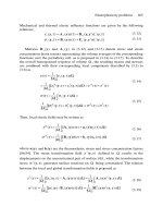
These equations are quite general for a beam of uniform
flexural stiffness
subjected to any concentrated load P acting at For instance, Equation (4.60) can
be used for a clamped-free beam with a load P acting at the tip of x = L by letting
Also because the equations evolve from linear theory, superposition can be used if
there are two concentrated loads at two different locations, but care must be used to
accurately depict regions to the left and right of each load to insure correct solutions.
After the solutions are found, Equations (4.14) and (4.17) are used to
obtain bending moments and shear resultants, and Equation (4.26) is used to determine
stresses everywhere.
4.4 Solutions by Green’s Functions
171
From Section 4.3, consider a composite beam subjected to a unit concentrated
load, i.e., P = 1. By way of example, consider the beam simply supported at each end
given by Equations (4.62) and (4.63). In this case,
Note that is the deflection to the left of the load, to the right of the load.
Green’s function and can be defined as the deflection at x due to a unit load at
It can be reasoned that any distributed load q(x
)
is in fact an
infinity
of
concentrated loads, which can be summed to obtain the solution of the response to a
distributed load. Because of the
infinity
of concentrated loads, the
infinite
summation

can be replaced by an integration such that the following is correct.
For a beam simply supported at each end Equations (4.66) and (4.67) would be
inserted for and and other analogous expressions from Section 4.3 would be used
for beams with other boundary conditions.
As an example, solving Equations (4.68), (4.66) and (4.67) with
uniform load over the entire length, results in
which is the solution obtained through solving the governing differential equation (4.20)
and satisfying the appropriate boundary conditions, with the explicit solution shown in
172
Equation (4.49). Likewise, using the Green’s function approach discussed above for a
uniform load results in Equation (4.29) for the clamped-clamped beam, and Equation
(4.37) for the cantilevered beam.
Thus, with the use of Green’s
functions
one uses an integral equation where the
Green’s functions satisfy the boundary conditions, rather than solving the governing
differential equation and matching boundary conditions. This alternative approach
1.
2.
is general for any governing differential equation such as a beam, plate or shell.
can save great computational difficulty for complicated problems.
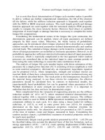
As an example of the latter, consider the following problem (Figure 4.7):
To solve the problem above, developing a solution requires solving the governing
differential equations and matching boundary conditions involves dividing the beam into
six sections, wherein twenty-four boundary value constants must be solved for, and
particular solutions obtained for each of the distributed loads. As a result, w
(
x
)
is

determined everywhere after all constants are solved for simultaneously.
Using the Green’s function approach, suppose that one hypothesizes that the
maximum deflection and bending moment occurs in the region One obtains
and for the clamped-simply supported beam from Equations (4.58)
and (4.59). Then for is given by
w
(
x
)
173
To check that the maxima occur in this region, one could easily investigate
adjoining regions, i.e., and Having obtained Equation (4.78),
maximum deflections and stresses are determined straightforwardly as shown before.
4.
5
Composite Beams of Continuously Varying Cross-Section
There are many applications in which beams can be better designed and utilized
through having a variable cross-section rather than a constant cross-section discussed in
Sections 4.1 through 4.4. In that case, the and are functions of x,
the length dimension, i.e., and
In that case, it is straightforward to derive the governing equation of beam
bending, analogous to the derivation leading to Equation (4.20). The result is
where here I
(
x
)
is a continuously varying function of x, and the mid-surface of the beam
is z = 0. Depending on what that function of x is, the solution could be rather
complicated and/or tedious.
For these types of problems, Galerkin’s method is well suited. No attempt is

made here to provide a detailed comprehensive introduction of Galerkin’s method, which
is well treated in numerous other texts. However, consider an ordinary differential
equation (although the method is equally useful for partial differential equations as well
as nonlinear equations).
where
L
is any differential operator, and q(x
)
is a forcing function. Boundary conditions
must be homogeneous; if not, a transformation of variables must be made first to attain
homogeneous boundary conditions.
In Galerkin’s method one assumes a complete set of coordinate functions
n = 1, 2, 3, , N, which satisfies the prescribed homogeneous boundary conditions.
Although these functions need not be an orthogonal set, if they are, the procedure is much
simpler. Therefore, assume
174
where the are constants.
By using only the first N terms, an error can be defined from Equations
(4.73) and (4.72), as
If is sufficiently small, then of Equation (4.73) is considered to be
a satisfactory approximation to w
(
x
)
. So can be viewed as an error function, and
the task is to select proper values of to minimize In the Galerkin method, this
is done by the following orthogonality condition:
This is equivalent to minimizing the mean square error and insures that
will converge to w
(

x
)
in the mean.
From above, this is equivalent to stating:
Therefore, Equation (4.76) is a set of N algebraic equations through which one
can determine the to minimize This is a powerful technique.
As an example, consider a tapered beam subjected to a lateral distributed load
q
(
x
)
, as developed by R.L. Daugherty when he taught a course using the first edition of
this text. Assume the variable stiffness can be written as:
Equation (4.71) can then be written as
where primes denote differentiation with respect to x. Hence,
175
If the beam is s
i
mply supported, i.e. ,
at x=0, L, coordinate functions
can be chosen as follows:
These are a complete set of functions, which satisfy the boundary conditions.
Thus,
and from Equation (4.74)
From Equations (4.75) and (4.76), Galerkin’s procedure requires
To continue the example, let f
(
x
)
= 1 +

(
x/ L
)
,
then Equation (4.83) becomes:
176
So Equation (4.82) is, for
For n = m
Thus, Equation (4.82) becomes for n = m
If N is taken as 3 for example, the final set of three non-homogeneous algebraic equations
are written as follows to obtain and The first, second and third equations are
for m = 1, 2, 3, respectively.
For
177
To complete the problem for any distributed load, q(x
)
, is straightforward.
To know what value of N to take can only be determined by solving the problem
with one higher integer and determining that the previous approximation is sufficient.
One thing to remember is that the result of this method is the determination of an
approximate deflection w(x). To determine stresses requires solving for since the
bending stresses are proportional to Taking derivatives of an approximative function
causes an increase in the error through differentiation. Hence, for stress critical structural
members, N must be determined by suitably approximate the maximum stress. This may
require a higher value of N than that required to achieve a certain accuracy in maximum
deflection.
4.6 Rods
Consider the rod shown in Figure 4.1 and 4.8 subjected to a uniform tensile axial
load in the
x

-direction.
One wishes to determine the in-plane mid-plane displacement and the axial
stresses in each lamina
The assumptions are:
a
.
Individual plies (laminae) are perfectly bonded (no slip).
178
b.
c.
d.
e.
f.
g.
h.
The thickness dimensions of the rod are small compared to the length of the rod.
Displacements and strains are small compared to all beam/rod dimensions.
A balanced, mid-plane symmetric laminate is used, i.e.,
The loading is static.
For simplicity of example hygrothermal effects are ignored.
The loading is in the x-z plane.
Since b << L, strains in the
y
-direction are ignored.
The governing equation for axial equilibrium is easily shown to be as follows,
where here an axial component has been added to (4.5)
where from Figure 4.8, p
(
x
)

is the axial distributed force per unit area, which can be a
function of x.
The mid-plane strain-axial displacement equation is again seen to be
The constitutive equation can be given by the following for each ply,
where is the ply stiffness in the x -direction of the kth lamina, and is equivalent to
if Poisson’s ratio effects are ignored.
It has been shown in many texts that can be written as follows:
where all quantities have been defined previously. *Note that as alternative to using
Equations (4.87) and (4.88) to obtain the stress in the
k
th lamina, one could use Equation
(4.19) where of course because with a beam
The integrated axial stress resultant is seen to be, as in (4.3)
Utilizing the above equations the governing differential equation is found to be
179
If the rod is held fixed at x = 0 in Figure 4.8, then the boundary conditions are:
The solution is found straightforwardly to be
and the stress in the kth lamina is
4.7 Vibration of Composite Beams
In Sections 4.1 through 4.5 the problems studied have concentrated on (1) finding
the maximum deflection in composite beams to insure that they are not too large for a
deflection-limited or stiffness-critical structure, and (2) determining the maximum
stresses in the beam structure for those structures, which are strength critical. However,
there are two other ways in which a structure can become damaged or useless; one is
through a dynamic response to time-dependent loads, and the other is through the
occurrence of an elastic instability (buckling).
In the former, dynamic loading on a structure can vary from a recurring cyclic
loading of the same repeated magnitude, such as a structure supporting an unbalanced
motor that is turning at a specified number of revolutions per minute (for example), to the
other extreme of a short time, intense, nonrecurring load, termed shock or impact loading,

such as a bird striking an aircraft component during flight. A continuous infinity of
dynamic loads exists between these extremes of harmonic oscillation and impact.
180
Whole volumes are written on the dynamic response of composite structures to
time-dependent loads, but that is beyond the scope of this text. There are a number of
texts dealing with dynamic response of isotropic structures. However, one common
thread to all dynamic responses are the natural frequencies of vibration and their
associated mode shapes.
Mathematically, any continuous structure has an infinity of natural frequencies
and mode shapes. If a structure is oscillated at a frequency that corresponds to a natural
frequency, it will respond by a rapidly growing amplitude with time, requiring very little
input energy, until such time as the structure becomes overstressed and fails, or until the
oscillations become so large that nonlinear effects may limit the amplitude to a large but
usually unsatisfactory value, and then considerable fatigue damage can occur.
Thus, to insure the structural integrity of any structure being designed or
analyzed, the natural frequencies should be determined in order to compare them with
any time-dependent loadings to which the structure will be subjected. This is to insure
that the frequencies imposed and the natural frequencies differ considerably. Conversely,
in designing a structure, over and above insuring that the structure will not over-deflect,
or become overstressed, care should be taken to avoid resonances (that is, imposed loads
having the same frequency as one or more natural frequencies).
The easiest example to illustrate this behavior is that of the bending of a beam
previously studied, with mid-plane symmetry so that there is no bending-
stretching coupling and no transverse shear deformation In this case the
governing equation (4.20), is repeated below:
In Equation (4.94), it is seen that the imposed static load is written as a force per
unit length. For dynamic loading, if d’Alembert’s Principle were used then one can add a
term to Equation (4.94) equal to the product mass and acceleration per unit length. In
that case Equation (4.94) becomes
where w and q both become functions of time as well as space, and derivatives therefore

become partial derivatives, is the mass density of the beam material, and here A is
the beam cross-sectional area. In the above, q
(
x,t
)
is now the spatially varying time-
dependent forcing function causing the dynamic response, and could be anything from a
harmonic oscillation to an intense one-time impact.
For a composite beam in which different laminae have differing mass densities,
then in the above equations use, for a beam of rectangular cross-section,
181
However, natural frequencies for the beam occur as functions of the material
properties and the geometry and hence are not affected by the forcing functions;
therefore, for this study let q
(
x,t
)
be zero. Thus Equation (4.94) becomes
One sees that this is the homogeneous equation associated with Equation (4.94).
For a simple case, (the easiest one) assume the composite beam to be simply supported at
each end. One may assume a spatial component of the lateral deflection to satisfy the
simply-supported boundary conditions, a harmonic temporal component, and an
amplitude such that
Here is called the natural circular frequency in radians per unit time for the
n
th
vibrational mode. Note that in this case there is one natural frequency for each natural
mode shape, for n = 1, 2, 3, , etc.
For this to be true, then by substituting Equation (4.98) into (4.97) and solving for
it is seen that for each value of n,

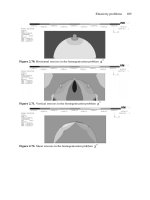
Thus, for each n there is a different natural frequency, and a different mode shape, as
shown in Figure 4.9.
For each value of n, the natural frequency is important because if the beam were
forced to oscillate at that particular frequency, a resonance would occur, and the
amplitude would grow until some form of structural failure would occur, as discussed
previously.
182
The lowest natural frequency, corresponding to n =
1
in this simply supported
beam case, is termed the fundamental frequency. It should be noted that n could go from
a value of one to infinity. However, the governing differential equation (4.97) is only
applicable over a portion of this range, i.e., it applies to those mode shapes in which the
classical beam equations apply. For an isotropic single-layer beam, the equation breaks
down when the half wavelength becomes close to the height, h, of the beam, because then
transverse shear deformation effects become important, and the classical theory
of Equations (4.94) and (4.97) yields increasingly inaccurate frequencies. In composite
material beams, transverse-shear deformation effects can be important even for the
fundamental natural frequency; but to include transverse shear deformation and rotatory
inertia effects involves considerable analytical complications, that will be dealt with later
in this chapter. Natural frequencies using classical beam theory, such as Equation (4.99)
for the case of both ends simply supported, are useful for preliminary design and forensic
analyses.
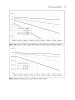
It is handy to know the natural frequencies of beams for various practical
boundary conditions in order to insure that no recurring forcing functions are close to any
of the natural frequencies, because that would result almost certainly in a structural
failure. In each case below, the natural circular frequency in radians/unit time are
given as
where all terms have been explained earlier except the coefficient Once is
known then the natural frequency in cycles per second (Hertz) is given by

183
The values of have been catalogued by Warburton [2], Young and Felgar [3] and
Felgar [4]. Some values are given in Table 4.1 for ease of use.
Incidentally, the natural frequencies of a free-free beam equal those of a clamped-
clamped beam. Also if transverse-shear deformation effects were included, each of the
above natural frequencies would be lower. This will be discussed later.
4.8
Beams With Mid-Plane Asymmetry
In considering a beam that is not mid-plane symmetric, the equilibrium equations
remain the same as given by Equations (4.5), (4.6) and (4.7).
However, because of mid-plane asymmetry, bending-stretching coupling occurs,
and therefore the extensional and bending behavior are coupled. From Equation (2.66) it
is seen that the constitutive equations for the asymmetric beam are
Likewise the in-plane and lateral displacements are given by the usual translation plus
rotation only for classical theory:
Proceeding as before for the symmetric beam the two coupled differential equations can
be written as follows:
184
where all terms have been explained previously except for . This term is a mid-plane
asymmetry parameter [5]. It is defined as
It is zero for a mid-plane symmetric structure, and it can be shown that physically
the limits of are
In (4.103) the term is the reduced flexural stiffness defined by
Whitney [6].
One then solves Equation (4.103) above analogous to the solutions for the mid-
plane symmetric beam.
For a beam that is subjected to a uniform load per unit length the maximum
deflection can be written as [7].
where values of are 12 for a clamped-clamped beam; 8 for a simple-simple beam and
2 for a cantilevered beam.

When considering mid-plane asymmetric beams, the asymmetry could be due to
using different composite materials for the upper and lower portions, which of course
would have different mechanical properties. Alternatively, even if the same composite is
used throughout the beam, there may be differing strengths and moduli in tension and
compression. So care must be taken to ensure the allowable stress is not exceeded either
in tension or compression.
4.9 Advanced Beam Theory for Dynamic Loading Including Mid-Plane Asymmetry
Consider the elasticity equilibrium equations in the x and z directions and the
moment equilibrium equations where now, using d’Alemberts’ Principle, the initial terms
are included. The results are, without derivation, where in this section p
(
x,t
)
is the axial
load per unit cross-sectional area, and q
(
x,t
)
is the lateral load per unit length of the beam.
185
where and are the longitudinal inertia, the bending-stretching coupling inertia
and the rotatory inertia respectively defined as:
where is the mass density of each ply, e.g. lb.
These equations can be simplified to the following coupled equations:
Making use of the constitutive equations of (2.66), and the strain displacement
relations, the following dynamic equations can be obtained in terms of the displacements:
186
If the loads are static, these equations become
Note, in the above the subscript T denotes thermal terms, and the subscript m denotes
moisture effects. represents the axial moment distribution.

Solving the first equation above for the function of which is then substituted
into the second equation, the result is:
One sees immediately that the reduced bending stiffness is
It is seen that if the beam is mid-plane symmetric, the last term on the right hand side of
Equation (4.119) is zero.
As an example, consider a mid-plane asymmetric beam simply supported at each
end, where there is a lateral load per unit length q
(
x
)
only. The above equations are
simply:
187
where
In this case the solution is:
In the beam simply supported at each end, with no axial load, and arbitrarily
setting the solution is:
Using now the following equations for the stress in the axial direction in the kth lamina
188
From the foregoing where Poisson’s ratio effects are ignored for a
beam. Thus, one finds that
From beam theory if one uses the relationship
one can conclude that
then from above
where is a negative number associated with the bottom of lamina 1, i.e., the lower
face of the beam.
Now for the specific case of (a constant).
189
and the stresses are
Now as an example problem consider the mid-plane asymmetric beam subjected

only to a static hygrothermal loading, and no mechanical loads.
From above, the governing differential equations are
Integrating these equations straightforwardly produces the solutions for the deflection.
where
190
For this example problem consider the beam to be simply supported at each end,
hence the boundary conditions are
The values of the seven constants are easily found to be
Therefore, for this case the displacements are seen to be
191
One general observation can be made: The thermal effects and the moisture
effects on this and every other structure are identical. So as long as one is using linear
theory, the two effects obviously are superposed as seen above. But the important thing
to remember is that if one has the thermal effect solution to any solid mechanics (linear,
problem, then through superposition one has the solution of the hygrothermal problem for
the same structure and boundary conditions.
Finally, consider the following numerical example. It provides the reader with the
opportunity to perform numerical calculations to insure that everything previously
discussed is understood.
Consider a beam of quasi-isotropic
laminate of E-glass/epoxy composite of width and ply thickness 0.01
inches. The composite mechanical properties are:
The axial mechanical properties are obtained from using
So
i.e., [0, +45, -45, 90, 90, -45,
+45, 0]
192
the axial coefficients of thermal expansion are given by
The thermal loadings are as follows
Finally, the deformations for this problem are

4.10 Advanced Beam Theory Including Transverse Shear Deformation Effects
193
The effects of transverse shear deformation are discussed now so that a
comparison can be made with the analyses of Section 4.8, which did not include these
effects. The development of this section includes dynamic mechanical and hygrothermal
loadings.
As stated previously, in almost all cases transverse shear deformation effects are
significant in composite material structures because in almost all cases the fibers, which
strengthen and stiffen the matrix are in the x-y plane, so the transverse shear stiffnesses
closely resemble the shear stiffness of the matrix material only, hence more compliant
than many in-plane properties.
The equilibrium equations can be written as
where
For the above, the deflections are still given as
The strain displacement relations are
194
The stress-strain relations are for each ply
The integrated constitutive equations are
where here is a transverse shear correction factor described previously. For the static
loading case, the governing equations are given as:
Substituting (4.158) into (4.160), and taking the first derivative of the result, results in
Now taking the second derivative of Equation (4.159) and substituting it into the above,
results in
Thus the right hand side of the above two equations can be written as