Computational Mechanics of Composite Materials part 5 ppt

Elasticity problems 105
Figure 2.70. Horizontal stresses in the homogenisation problem
11
Figure 2.71. Vertical stresses in the homogenisation problem
11
Figure 2.72. Shear stresses in the homogenisation problem
11
106 Computational Mechanics of Composite Materials
Figure 2.73. Vortex visualization of the homogenisation function
11
Figure 2.74. Relative error of the stresses determination in the problem
11
Figure 2.75. Relative error for strain determination in the homogenisation problem
11
Elasticity problems 107
Figure 2.76. Relative error of the strain energy determination
11
Figure 2.77. Horizontal components of the homogenisation function
12
Figure 2.78. Vertical components of the homogenisation function
12
108 Computational Mechanics of Composite Materials
Figure 2.79. Total values of the homogenisation function
12
Figure 2.80. Horizontal stresses in the homogenisation problem
12
Figure 2.81. Vertical stresses in the homogenisation problem
12
Elasticity problems 109
Figure 2.82. Shear stresses in the homogenisation problem
12

Figure 2.83. Equivalent von Mises stresses in the homogenisation problem
12
Figure 2.84. Vortex visualization of the homogenisation function
12
110 Computational Mechanics of Composite Materials
Figure 2.85. Relative error of the stresses determination in the problem
12
Figure 2.86. Relative error of the strain determination in the problem
12
Figure 2.87. Relative error of the strain energy determination
12
Elasticity problems 111
Figure 2.88. Horizontal components of the homogenisation function
22
Figure 2.89. Vertical components of the homogenisation function
22
Figure 2.90. Total values of the homogenisation function
22
112 Computational Mechanics of Composite Materials
Figure 2.91. Horizontal stresses in the homogenisation problem
22
Figure 2.92. Vertical stresses in the homogenisation problem
22
Figure 2.93. Shear stresses in the homogenisation problem
22
Elasticity problems 113
Figure 2.94. Vortex visualization of the homogenisation function
22
Figure 2.95. Relative error of the stresses determination in the problem
22

Figure 2.96. Relative error of the strain determination in the problem
22
114 Computational Mechanics of Composite Materials
Figure 2.97. Relative error of the strain energy determination
22
The results of the computational analysis carried out in this section show that
the effective properties of the composite and, at the same time, the overall
behaviour of the composite, in the context of the homogenisation method, are
sensitive to the interphase between the constituents and its material parameters. It
should be underlined that the interphase, improved in the example presented above,
has small total area in the comparison to the fibre and matrix. It can be expected
that the previous, simplified approach (upper and lower bounds or direct
approximations of effective properties cited above) do not enable us to arrive at
such effects.
Considering the assumption that the scale factor between the RVE and the
whole composite structure tends to 0 in our analysis and, on the other hand, that
this quantity in real composites is small but differs from 0, the sensitivity of the
effective characteristics to this parameter are to be calculated in the next analyses
based on this approach. To carry out such studies, the scale parameter has to be
introduced in the equations describing effective properties and next, due to the
well-known sensitivity analysis methods, the influence of the scale parameter ε
relating composite micro and macrostructure may be shown. In the analogous
way we can study the sensitivity of the effective characteristics of the composite to
the component material parameters but there is no need in this case to introduce
any extra components into the equations cited above.
Further mathematical and computational extensions of the model presented
should be provided to include in the constitutive tensor the components responsible
for the thermal expansion [228,311]. Having computed the effective characteristics
on the basis of Young moduli, Poisson ratios, coefficient of thermal expansion and
heat conduction coefficient [106,163,347] it will be possible to provide the coupled

temperature displacement FE analyses of periodic composite materials. At the
same time it will be valuable to work out the problem presented in the context of
viscoelastic or elastoviscoplastic material models of the composite constituents
[74,368]. It will enable us to approximate computationally the fracture and failure
phenomena in composites resulting from the interface defects or partial debonding
using the homogenisation approach.
Elasticity problems 115
2.3.3.2.2 Monte Carlo Simulation Analysis
Starting from the formula describing the effective elasticity tensor components,
their expected values are derived using the basic theorems on the random variables
as follows [191]:
[]
[]
Ω
Ω
+
⎥
⎦
⎤
⎢
⎣
⎡
= );();(();(
)(
ωωχσω
xCExExCE
ijkl
ij
kl
eff

ijkl
(2.167)
The expressions for the variances (and generally covariances) have a more
complicated form than the expectations because the averaged stresses and elasticity
tensor are correlated variables. Therefore
()
()
ΩΩ
Ω
Ω
+
⎟
⎠
⎞
⎜
⎝
⎛
+
⎟
⎠
⎞
⎜
⎝
⎛
=
);();(,);((2
);(();(
)(
ωωωχσ
ωχσω

xCVarxCxCov
xVarxCVar
ijklijkl
ij
kl
ij
kl
eff
ijkl
(2.168)
The random homogenisation fields ),(
ωχ
x
ij
for general composites, similar to
the deterministic ones, are calculated only numerically. The following probabilistic
stress boundary conditions are imposed on the boundary
),1( aa−
Γ to find the
homogenisation functions:
()
⎥
⎦
⎤
⎢
⎣
⎡
++
⎥
⎦

⎤
⎢
⎣
⎡
=
⎥
⎦
⎤
⎢
⎣
⎡
−−
−
ΓΓ
Γ
piqqipipq
ipq
nnEnE
FE
aaaa
aa
δδωµδωλ
ω
),1(),1(
),1(
)()(
)(
)(
(2.169)
()

⎟
⎠
⎞
⎜
⎝
⎛
++
⎟
⎠
⎞
⎜
⎝
⎛
=
⎟
⎠
⎞
⎜
⎝
⎛
−−
−
ΓΓ
Γ
piqqipipq
ipq
nnVarnVar
FVar
aaaa
aa

δδωµδωλ
ω
),1(),1(
),1(
)()(
)(
)(
(2.170)
where λ(ω) and µ(ω) are the Lame constants. If Young moduli of composite
components are considered as input random variables then the expected values and
variances of boundary forces are obtained by separating the RHS into those
components corresponding to
1−
Ω
a
and
a
Ω , respectively. After some algebraic
transformations there holds
[
]
[] [ ]
11)(
)()();(
−−
⋅−⋅=
aapqiaapqiipq
eEBeEBxFE
ννω
(2.171)

116 Computational Mechanics of Composite Materials
where the operator ))(( x
ν
pqi
B similar to the tensor introduced by eqn (2.14)
is defined as
))(1(2
1
)(
))(21))((1(
)(
))((
xxx
x
x
ν
δδ
νν
ν
δν
+
++
−+
=
piqqipipqpqi
nnnB
(2.172)
and their variances are equal to
(){}
()

{}
()
1
2
1
2
)(
)()();(
−−
⋅+⋅=
aapqiaapqiipq
eVarBeVarBFVar
ννω
x
(no sum on p,q,i)
(2.173)
Finally, probabilistic moments of the effective characteristics are derived using
statistical estimation methods, according to which the expected values and the
relevant covariances (computed using the unbiased estimator) of the effective
elasticity tensor components are obtained as
[]
∑
=
=
M
j
jeff
ijpq
M
eff

ijpq
CCE
1
)(
1
)(
(2.174)
()
[]
()
[]
()
)()(
1
)()(
1
)()(
)(),(
eff
rsuv
jeff
rsuv
M
j
eff
ijpq
jeff
ijpq
M
eff

rsuv
eff
ijpq
CECCECCCCov −−=
∑
=
ωω
(2.175)
where
()
ω
jeff
ijpq
C
)(
, Mj , ,1= are random series of the tensor components obtained
as a result of the generation of numerical random values.
The homogenisation problem presented is implemented into the program
MCCEFF, which is based on the Monte Carlo simulation technique. The
implementation of the MCS has been selected from among many other
probabilistic methods, because this method consists of computer generation of
random variables in the mechanical problem (cf. Figure 2.98) and computing the
sequence of deterministic solutions associated with each variable generated;
similar engineering software is also available [47]. Considering the fact that a
composite structure has a relatively small number of degrees of freedom, a crude
random sampling method is used in the computations (contrary to the Random
Importance or Stratified Sampling methods) [73,125,139].
Define N, m, a, c, E[e], σ(e), E[
ν
], σ(

ν
)
↓
Generate uniform distribution
{}
)1,0(, ,
1
−∈ mII
N
Do for k=1,N
)(mod
1
mcaII
kk
+=
−
Enndo
↓
Elasticity problems 117
Transform I→x: uniform distribution on (0,1)
Scaling distribution {I} by the parameter m
↓
Transform pairwise (x
i
,x
i+1
)→(y
i
,y
i+1

): N(0,1)
Do for i=1,N
⎪
⎩
⎪
⎨
⎧
−=
−=
++
+
11
1
2sinln2
2cosln2
iii
iii
xxy
xxy
π
π
Enddo
↓
Transform y→e,
ν
Do for i=1,N
e
i
=E[e]+y
i

σ(e);
ν
i
=E[
ν
]+y
i
σ(
ν
)
Enddo
↓
Cutting off e,
ν
distributions
Verify for i=1,N
()
trueeS =∞<<0
1
;
()
trueS =<<−
2
1
2
1
ν
Enddo
↓
Computations of the total sample length

M=N-K: K=sup(k1,k2);
k
1
,k
2
- number of S1,S2 negations
Figure 2.98. Algorithm for random numbers generation
However, the most important reason for the MCS application is that the
accuracy of the output variable probabilistic moments estimation does not depend
on the input variable coefficient of variation (as for the SFEM), but on the total
number of iterations performed. Taking into account the estimator convergence
studies and some theoretical considerations, the total number of random trials M
has been taken as equal to 1,000. The flowchart of the program used for
probabilistic homogenisation is shown in Figure 2.99. As presented, the program
makes it possible to discretise automatically the RVE on the basis of the main cell
geometrical parameters, visualisation of the mesh introduced, random generation
of the input random variables and iterative computations of the homogenisation
functions as well as statistical estimators of either upper and lower bounds or direct
effective characteristics of the elasticity tensor components.
Automatic-parametric mesh generator
↓
Input data visualization
↓
1st loop over random spaces
Do for iter=1,M
Generation of
()
ω
e
,

()
ων
118 Computational Mechanics of Composite Materials
Enddo
Computations of PDFs of elasticity tensor components
Upper and lower bounds:
()
()
ω
)(
sup
eff
ijkl
C ,
()
()
ω
)(
inf
eff
ijkl
C
2nd loop over random spaces
Do for iter=1,M
Generation of )(
)(
ω
ipq
F
Enddo

↓
3rd loop over random spaces
Do for iter=1,M
Homogenisation plane strain problems
()
ωχ
;
)(
x
ipq
,
()
Ω
⎟
⎠
⎞
⎜
⎝
⎛
ωχσ ;
i)pq(kl
x
()
ω
;
)(
x
eff
ijkl
C

Enddo
↓
4th loop over random spaces
do for iter=1,M
Computations of statistical estimators
(
)
)(eff
ijkl
p
C
µ
,
(
)
(
)
)(
sup
eff
ijkl
p
C
µ
,
(
)
(
)
)(

inf
eff
ijkl
p
C
µ
()()
)(
sup
eff
ijkl
CPDF
,
()
)(eff
ijkl
CPDF
,
()()
)(
inf
eff
ijkl
CPDF
Enddo
Figure 2.99. Algorithm for the MCS simulation of homogenisation procedure
Numerical analysis of probabilistic homogenisation of the fibre composite with
stochastic interface defects has been performed using the MCCEFF system
described above. Internal automatic generator for the square RVE with a centrally
located round fibre occupying about 50% of the RVE with interface defects has

been used (the influence of fibre radius variation on the stochastic displacements
and stress fields has been discussed previously). Considering greater composite
sensitivity to the matrix defects (bubbles), only composites having such
discontinuities have been homogenised. The elastic constants for the fibre material
have been taken as follows:
[]
1
eE =84 GPa, ν
1
=0.22 and the coefficient of Young
modulus variation
()
1
e
α
=0.1, and for matrix:
[]
2
eE =4 GPa,
2
ν
=0.34. Interface
defect parameters have been taken in such a way that the coefficients of variation
of these parameters were equal to 0.1 in all tests:
()
][1.0 rEr ⋅=
σ
and
()
][1.0 nEn ⋅=

σ
.
The main aim of the numerical experiments performed was a numerical
verification of the presented mathematical approach to homogenisation of
composites with stochastic interface defects. Considering large number of
Elasticity problems 119
parameters in this approach it was necessary to analyse the probabilistic sensitivity
of the effective elasticity tensor components. It was done with respect to the
expected values of the interface defect number and volume and the coefficient of
matrix Young moduli variation as design parameters. Finally, 132 simulations have
been performed (with 1000 iterations each) with the following remaining input
values: E[r]=R{0.03,0.04,0.05} and E[n] has been assumed as equivalent to the
percentage ratio of the boundary where the defects are located to the total interface
length from 10% to 60% every 5%. The coefficient of matrix Young modulus
variation for tests No 1 4 has been taken as 0.100, 0.075, 0.050, 0.025,
respectively.
Probabilistic moments of the effective elasticity tensor obtained as a result of
the simulations are compared in Figures 2.100 2.119. The expected values of
)(
)(
1111
ω
eff
C are shown in such a way that the test results are presented in increasing
order in the relevant figures. The coefficients of variation of )(
)(
1212
ω
eff
C are

neglected in the sensitivity analysis because this random variable is a function of
random fluctuations of the fibre Young modulus. In all the collected figures the
ratio of interface discontinuities (DB) to the entire boundary is marked on the
horizontal axes, while the expected values
[]
)(
)(
ω
eff
ijkl
CE or the coefficients of
variation
()
)(
)(
ωα
eff
ijkl
C are displayed on the vertical axes, respectively.
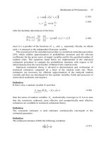
A decrease of the expected values of )(
)(
ω
eff
ijkl
C with an increase of the interface
defects number is observed with generally small differences in comparison with
the composite with perfect interface. For an increase of the parameter DB from
10% to 60%, the decrease considered is about 10% for
[]
)(

)(
1111
ω
eff
CE and
[]
)(
)(
1122
ω
eff
CE components, while for
[]
)(
)(
1212
ω
eff
CE it is only 1%. The low sensitivity
of the values for
[]
)(
)(
ω
eff
ijkl
CE obtained with respect to the coefficient of the matrix
Young modulus variation seems to be very important, as well. Moreover, it can be
noted that for an increase of the expected values of the interface defects, the values
of

[]
)(
)(
1111
ω
eff
CE and
[]
)(
)(
1122
ω
eff
CE increase too, and
[]
)(
)(
1212
ω
eff
CE decreases.
Finally, the increasing DB implies a decrease in the differences of
[]
)(
)(
1111
ω
eff
CE and
[]

)(
)(
1122
ω
eff
CE obtained for different defects values, while for
[]
)(
)(
1212
ω
eff
CE these
differences increase with the increasing total number of the defects.
120 Computational Mechanics of Composite Materials
Figure 2.100. Expected values
[]
)(
)(
1111
ω
eff
CE in test 1
Figure 2.101. Expected values
[]
)(
)(
1111
ω
eff

CE in test 2
Figure 2.102. Expected values
[]
)(
)(
1111
ω
eff
CE in test 3
Elasticity problems 121
Figure 2.103. Expected values
[]
)(
)(
1111
ω
eff
CE in test 4
Figure 2.104. Expected values
[]
)(
)(
1122
ω
eff
CE in test 1
Figure 2.105. Expected values
[]
)(
)(

1122
ω
eff
CE in test 2
122 Computational Mechanics of Composite Materials
Figure 2.106. Expected values
[]
)(
)(
1122
ω
eff
CE in test 3
Figure 2.107. Expected values
[]
)(
)(
1122
ω
eff
CE in test 4
Figure 2.108. Expected values
[]
)(
)(
1212
ω
eff
CE in test 1
Elasticity problems 123

Figure 2.109. Expected values
[]
)(
)(
1212
ω
eff
CE in test 2
Figure 2.110. Expected values
[]
)(
)(
1212
ω
eff
CE in test 3
Figure 2.111. Expected values
[]
)(
)(
1212
ω
eff
CE in test 4
124 Computational Mechanics of Composite Materials
Figure 2.112. Coefficients of variation
()
)(
)(
1111

ωα
eff
C in test 1
Figure 2.113. Coefficients of variation
()
)(
)(
1111
ωα
eff
C in test 2
Figure 2.114. Coefficients of variation
()
)(
)(
1111
ωα
eff
C in test 3
Elasticity problems 125
Figure 2.115. Coefficients of variation
()
)(
)(
1111
ωα
eff
C in test 4
Figure 2.116. Coefficients of variation
()

)(
)(
1122
ωα
eff
C in test 1
Figure 2.117. Coefficients of variation
()
)(
)(
1122
ωα
eff
C in test 2
126 Computational Mechanics of Composite Materials
Figure 2.118. Coefficients of variation
()
)(
)(
1122
ωα
eff
C in test 3
Figure 2.119. Coefficients of variation
()
)(
)(
1122
ωα
eff

C in test 4
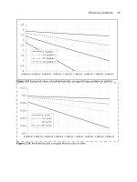
Analysing the coefficients of variation
()
)(
)(
ωα
eff
ijkl
C , a nonlinear increase of
these coefficients with a DB increase can be observed in all tests. This dependence
has a character similar to the behaviour of the coefficient of variation of the Young
modulus obtained during the interphase probabilistic averaging. Moreover, all
results are in the range of [0.00,0.12] for all the numerical tests, being negligibly
greater than the maximum value of the input parameter
()
2
e
α
. Furthermore, the
correlation of interface defect value increases and an
()
)(
)(
ωα
eff
ijkl
C increase is
observed, and in opposition to the expected values, the coefficients of the
)(
)(

ω
eff
ijkl
C tensor variation are sensitive to
()
2
e
α
changes. Together with the
decreasing coefficients of the matrix Young modulus variation the following
changes are observed:
decrease of
()
)(
)(
1111
ωα
eff
C and
()
)(
)(
1122
ωα
eff
C ;
Elasticity problems 127
increase of differences between these coefficients obtained for particular values
of interface defects;
significantly faster increase of

()
)(
)(
ωα
eff
ijkl
C (from 10% in test no 1 to about 30%
in test no 4).
The coefficients
()
)(
)(
1212
ωα
eff
C (not considered in the analysis) show total non-
sensitivity to analysed parameters.
Further, taking into account that all the results obtained from the Monte Carlo
simulations, e.g. the first two probabilistic moments of the effective elasticity
tensor, are only statistical estimators of the real values of these parameters, the
numerical sensitivity of these estimators to the number of iterations should be
analysed. Such an analysis is performed on the periodicity cell taking the total
number of random trials as N=5, 10, 25, 50, 100, 250, 500, 1000, 2500, 5000 and
10000, respectively.
Only the probabilistic parameters of )(
)(
1111
ω
eff
C are shown, because variations of

the other component moments of )(
)(
ω
eff
ijkl
C are quite similar to those presented.
The total numbers of random number sampling are marked on the horizontal axes,
while the analysed values of )(
)(
ω
eff
ijkl
C are on the vertical axes. The functions
describing convergence of particular estimators obtained in the numerical
experiments enable us to verify the correctness of the simulations performed and
come up with an optimum number of the samples for estimation of any
probabilistic coefficient and/or moment for the tensor )(
)(
ω
eff
ijkl
C .
Figure 2.120. Statistical convergence of the expected value
[]
)(
)(
1111
ω
eff
CE

128 Computational Mechanics of Composite Materials
Figure 2.121. Statistical convergence of the expected value
[]
)(
)(
1122
ω
eff
CE
Figure 2.122. Statistical convergence of the expected value
[]
)(
)(
1212
ω
eff
CE
Figure 2.123. Statistical convergence of coefficient of variation
()
)(
)(
1111
ωα
eff
C
Elasticity problems 129
Figure 2.124. Statistical convergence of coefficient of variation
()
)(
)(

1122
ωα
eff
C
Figure 2.125. Statistical convergence of coefficient of variation
()
)(
)(
1212
ωα
eff
C
It is seen from the analysis of the expected values of )(
)(
ω
eff
ijkl
C that the
estimator convergence character is described by a curve of similar shape in all the
tests. This curve gradually increases from a minimum at N=5 to a maximum at
about N=30 to oscillate with asymptotic convergence to the value approximated. It
is important that in practice for N=100 estimator gives quite a good estimation with
satisfactory accuracy. Taking for example N=1000, computational error resulting
from statistical estimation is negligibly small in comparison with the estimated
value.
Convergence of
()
)(
)(
ωα

eff
ijkl
C estimators has quite a different character than for
[]
)(
)(
ω
eff
ijkl
CE estimators described above. From the maximum obtained for N=5 the
curve describing the estimator as a function of the total number of iterations
decreases between two inflection points for about N=10 and N=30, then for about
N=100 it starts to converge asymptotically to the approximated quantity.
Analogous to the expected values the shape of the analysed curves is quite similar