Volume 08 - Mechanical Testing and Evaluation Part 5 pot

Table 12 Approximate equivalent hardness numbers for wrought coppers (>99% Cu, alloys C10200 through C14200)
Vickers
hardness
No.
Knoop
hardness No.
Rockwell superficial hardness No. Rockwell hardness
No.
Rockwell superficial hardness No. Brinell hardness
No.
1
kgf,
HV
100
gf,
HV
1
kgf,
HK
500
gf,
HK
15T scale,
15
kgf, in.
(1.588
mm)
ball,
HR15T
(a)

15T scale,
15
kgf, in.
(1.588
mm)
ball,
HR15T
(b)

30T scale,
30
kgf, in.
(1.588
mm)
ball,
HR30T
(b)

B scale,
100
kgf,
in.
(1.588
mm)
ball,
HRB
(c)

F scale,
60 kgf,

in.
(1.588
mm)
ball,
HRF
(c)

15T scale,
15 kgf,
in.
(1.588
mm)
ball,
HR15T
(c)

30T scale,
30 kgf,
in.
(1.588
mm)
ball,
HR30T
(c)

45T scale,
45 kgf,
in.
(1.588
mm)

ball,
HR45T
(c)

500 kgf,
10
mm
diam
ball,
HBS
(d)

20 kgf,
2 mm
diam
ball,
HBS
(e)

130 127.0 138.7

133.8 … 85.0 … 67.0 99.0 … 69.5 49.0 … 119.0
128 125.2 136.8

132.1 83.0 84.5 … 66.0 98.0 87.0 68.5 48.0 … 117.5
126 123.6 134.9

130.4 … 84.0 … 65.0 97.0 … 67.5 46.5 120.0 115.0
124 121.9 133.0

128.7 82.5 83.5 … 64.0 96.0 86.0 66.5 45.0 117.5 113.0
122 121.1 131.0

127.0 … 83.0 … 62.5 95.5 85.5 66.0 44.0 115.0 111.0
120 118.5 129.0

125.2 82.0 82.5 … 61.0 95.0 … 65.0 42.5 112.0 109.0
118 116.8 127.1

123.5 81.5 … … 59.5 94.0 85.0 64.0 41.0 110.0 107.5
116 115.0 125.1

121.7 … 82.0 … 58.5 93.0 … 63.0 40.0 107.0 105.5
114 113.5 123.2

119.9 81.0 81.5 … 57.0 92.5 84.5 62.0 38.5 105.0 103.5
112 111.8 121.4

118.1 80.5 81.0 … 55.0 91.5 … 61.0 37.0 102.0 102.0
110 109.9 119.5

116.3 80.0 … … 53.5 91.0 84.0 60.0 36.0 99.5 100.0
108 108.3 117.5

114.5 … 80.5 … 52.0 90.5 83.5 59.0 34.5 97.0 98.0
106 106.6 115.6

112.6 79.5 80.0 … 50.0 89.5 … 58.0 33.0 94.5 96.0
104 104.9 113.5

110.1 79.0 79.5 … 48.0 88.5 83.0 57.0 32.0 92.0 94.0
102 103.2 111.5

108.0 78.5 79.0 … 46.5 87.5 82.5 56.0 30.0 89.5 92.0
100 101.5 109.4

106.0 78.0 78.0 … 44.5 87.0 82.0 55.0 28.5 87.0 90.0
98 99.8 107.3

104.0 77.5 77.5 … 42.0 85.5 81.0 53.5 26.5 84.5 88.0
96 98.0 105.3

102.1 77.0 77.0 … 40.0 84.5 80.5 52.0 25.5 82.0 86.5
94 96.4 103.2

100.0 76.5 76.5 … 38.0 83.0 80.0 51.0 23.0 79.5 85.0
92 94.7 101.0

98.0 76.0 75.5 … 35.5 82.0 79.0 49.0 21.0 77.0 83.0
90 93.0 98.9 96.0 75.5 75.0 … 33.0 81.0 78.0 47.5 19.0 74.5 81.0
88 91.2 96.9 94.0 75.0 74.5 … 30.5 79.5 77.0 46.0 16.5 … 79.0
86 89.7 95.5 92.0 74.5 73.5 … 28.0 78.0 76.0 44.0 14.0 … 77.0
84 87.9 92.3 90.0 74.0 73.0 … 25.5 76.5 75.0 43.0 12.0 … 75.0
82 86.1 90.1 87.9 73.5 72.0 … 23.0 74.5 74.5 41.0 9.5 … 73.0
80 84.5 87.9 86.0 72.5 71.0 … 20.0 73.0 73.5 39.5 7.0 … 71.5
78 82.8 85.7 84.0 72.0 70.0 … 17.0 71.0 72.5 37.5 5.0 … 69.5
76 81.0 83.5 81.9 71.5 69.5 … 14.5 69.0 71.5 36.0 2.0 … 67.5
74 79.2 81.1 79.9 71.0 68.5 … 11.5 67.5 70.0 34.0 … … 66.0
72 77.6 78.9 78.7 70.0 67.5 … 8.5 66.0 69.0 32.0 … … 64.0
70 75.8 76.8 76.6 69.5 66.5 … 5.0 64.0 67.5 30.0 … … 62.0

68 74.3 74.1 74.4 69.0 65.5 … 2.0 62.0 66.0 28.0 … … 60.5
66 72.6 71.9 71.9 68.0 64.5 … … 60.0 64.5 25.5 … … 58.5
64 70.9 69.5 70.0 67.5 63.5 … … 58.0 63.5 23.5 … … 57.0
62 69.1 67.0 67.9 66.5 62.0 … … 56.0 61.0 21.0 … … 55.0
60 67.5 64.6 65.9 66.0 61.0 … … 54.0 59.0 18.0 … … 53.0
58 65.8 62.0 63.8 65.0 60.0 … … 51.5 57.0 15.5 … … 51.5
56 64.0 59.8 61.8 64.5 58.5 … … 49.0 55.0 13.0 … … 49.5
54 62.3 57.4 59.5 63.5 57.5 … … 47.0 53.0 10.0 … … 48.0
52 60.7 55.0 57.2 63.0 56.0 … … 44.0 51.5 7.5 … … 46.5
50 58.9 52.8 55.0 62.0 55.0 … … 41.5 49.5 4.5 … … 44.5
48 57.3 50.3 52.7 61.0 53.5 … … 39.0 47.5 1.5 … … 42.0
46 55.8 48.0 50.2 60.5 52.0 … … 36.0 45.0 … … … 41.0
44 53.9 45.9 47.8 59.5 51.0 … … 33.5 43.0 … … … …
42 52.2 43.7 45.2 58.5 49.5 … … 30.5 41.0 … … … …
40 51.3 40.2 42.8 57.5 48.0 … … 28.0 38.5 … … … …
(a) For 0.010 in. (0.25 mm) strip.
(b) For 0.020 in. (0.51 mm) strip.
(c) For 0.040 in. (1.02 mm) strip and greater.
(d) For 0.080 in. (2.03 mm) strip.
(e) For 0.040 in. (1.02 mm) strip.
Source: ASTM E 140 (Ref 6)
Table 13 Approximate equivalent hardness numbers for cartridge brass (70% Cu, 30%
Zn)
Rockwell hardness No. Rockwell superficial hardness No. Vickers
hardness
No., HV
B scale, 100
kgf, in.
(1.588 mm)
ball, HRF

F scale, 60
kgf, in.
(1.588 mm)
ball, HRF
15T scale,
15 kgf,
in.
(1.588 mm)
ball, HR15T
30T scale,
30 kgf,
in.
(1.588 mm)
ball, HR30T
45T scale,
45 kgf,
in.
(1.588 mm)
ball, HR45T
Brinell
hardness No.
500 kgf, 10
mm ball,
HBS
196 93.5 110.0 90.0 77.5 66.0 169
194 … 109.5 … … 65.5 167
192 93.0 … … 77.0 65.0 166
190 92.5 109.0 … 76.5 64.5 164
188 92.0 … 89.5 … 64.0 162
186 91.5 108.5 … 76.0 63.5 161

184 91.0 … … 75.5 63.0 159
182 90.5 108.0 89.0 … 62.5 157
180 90.0 107.5 … 75.0 62.0 156
178 89.0 … … 74.5 61.5 154
176 88.5 107.0 … … 61.0 152
174 88.0 … 88.5 74.0 60.5 150
172 87.5 106.5 … 73.5 60.0 149
170 87.0 … … … 59.5 147
168 86.0 106.0 88.0 73.0 59.0 146
166 85.5 … … 72.5 58.5 144
164 85.0 105.5 … 72.0 58.0 142
162 84.0 105.0 87.5 … 57.5 141
160 83.5 … … 71.5 56.5 139
158 83.0 104.5 … 71.0 56.0 138
156 82.0 104.0 87.0 70.5 55.5 136
154 81.5 103.5 … 70.0 54.5 135
152 80.5 103.0 … … 54.0 133
150 80.0 … 86.5 69.5 53.5 131
148 79.0 102.5 … 69.0 53.0 129
146 78.0 102.0 … 68.5 52.5 128
144 77.5 101.5 86.0 68.0 51.5 126
142 77.0 101.0 … 67.5 51.0 124
140 76.0 100.5 85.5 67.0 50.0 122
138 75.0 100.0 … 66.5 49.0 121
136 74.5 99.5 85.0 66.0 48.0 120
134 73.5 99.0 … 65.5 47.5 118
132 73.0 98.5 84.5 65.0 46.5 116
130 72.0 98.0 84.0 64.5 45.5 114
128 71.0 97.5 … 63.5 45.0 113
126 70.0 97.0 83.5 63.0 44.0 112

124 69.0 96.5 … 62.5 43.0 110
122 68.0 96.0 83.0 62.0 42.0 108
120 67.0 95.5 … 61.0 41.0 106
118 66.0 95.0 82.5 60.5 40.0 105
116 65.0 94.5 82.0 60.0 39.0 103
114 64.0 94.0 81.5 59.5 38.0 101
112 63.0 93.0 81.0 58.5 37.0 99
110 62.0 92.6 80.5 58.0 35.5 97
108 61.0 92.0 … 57.0 34.5 95
106 59.5 91.2 80.0 56.0 33.0 94
104 58.0 90.5 79.5 55.0 32.0 92
102 57.0 89.8 79.0 54.5 30.5 90
100 56.0 89.0 78.5 53.5 29.5 88
98 54.0 88.0 78.0 52.5 28.0 86
96 53.0 87.2 77.5 51.5 26.5 85
94 51.0 86.3 77.0 50.5 24.5 83
92 49.5 85.4 76.5 49.0 23.0 82
90 47.5 84.4 75.5 48.0 21.0 80
88 46.0 83.5 75.0 47.0 19.0 79
86 44.0 82.3 74.5 45.5 17.0 77
84 42.0 81.2 73.5 44.0 14.5 76
82 40.0 80.0 73.0 43.0 12.5 74
80 37.5 78.6 72.0 41.0 10.0 72
78 35.0 77.4 71.5 39.5 7.5 70
76 32.5 76.0 70.5 38.0 4.5 68
74 30.0 74.8 70.0 36.0 1.0 66
72 27.5 73.2 69.0 34.0 … 64
70 24.5 71.8 68.0 32.0 … 63
68 21.5 70.0 67.0 30.0 … 62
66 18.5 68.5 66.0 28.0 … 61

64 15.5 66.8 65.0 25.5 … 59
62 12.5 65.0 63.5 23.0 … 57
60 10.0 62.5 62.5 … … 55
58 … 61.0 61.0 18.0 … 53
56 … 58.8 60.0 15.0 … 52
54 … 56.5 58.5 12.0 … 50
52 … 53.5 57.0 … … 48
50 … 50.5 55.5 … … 47
49 … 49.0 54.5 … … 46
48 … 47.0 53.5 … … 45
47 … 45.0 … … … 44
46 … 43.0 … … … 43
45 … 40.0 … … … 42
Source: ASTM E 140 (Ref 6)
Magnesium and magnesium alloys are tested by applying the Rockwell B scale, but when the alloys are softer
(annealed), the indenter size is increased to 3.175 mm (⅛ in.) using the Rockwell E scale. As with other metals
and alloys, thin sections of magnesium alloys must be tested with the 15T or 30T scale to avoid the anvil effect.
Titanium. The Rockwell A scale is best suited for testing titanium. The 60 kgf load tends to increase the life of
the diamond penetrator because there is an affinity between diamond and titanium, which usually shortens
diamond life. Titanium tends to adhere to the tip of the diamond penetrator and can readily be removed with 3/0
grade emery paper when the penetrator is rotated in a lathe. Maintaining a clean diamond will give more
reliable results.
Zinc and lead alloys are typically tested using the Rockwell method. They exhibit extensive time-dependent
plasticity characteristics and therefore require longer dwell time of load application to obtain accurate and
repeatable results. For materials that show some time-dependent plasticity, the dwell time of indent load should
be 5 to 6 s using a diamond indenter. For materials that show considerable time-dependent plasticity, dwell time
should be 20 to 25 s using any indenter. One method for determining the magnitude of time-dependent
plasticity is to do a series of tests at progressively longer dwell times. As the dwell increases the hardness
values will decrease significantly. When the rate of change decreases significantly the proper dwell time has
been reached.

Zinc. The Rockwell E scale is used for zinc sheets down to 3.2 mm (0.125 in.) and the Rockwell H scale for
sheets down to 1.25 mm (0.050 in.) gage. These values are for zinc in the soft condition, thinner sheets may be
tested if the zinc is relatively hard. For thinner sheet, the 15T or 30T scale of the Rockwell superficial tester
should be used.
Lead. Most testing on lead is done on thicker specimens with the Rockwell E and H scales.
Tin plate is tested on the Rockwell superficial HR15T, HR30T, and HR45T scales along with a diamond spot
anvil in accordance with the following criteria:
Thickness
mm in.
Scale
<0.212 <0.0083 HR15T

0.213–0.547

0.0084–0.0215

HR30T

0.548–0.770

0.0216–0.0303

HR45T

Since most results are reported in the HR30T scales, all test results in the other scales are converted using the
standard conversion chart found in ASTM E 140 (Ref 6).
Cemented carbides are tested primarily with the Rockwell A scale as designated in ASTM B 294 (Ref 7). Using
the Rockwell C scale has resulted in poor diamond longevity due to breakage. Because of the extremely high
stress placed on the diamond point, only indenters designated for carbide testing should be used. It should be
noted that the carbide Rockwell A scale hardness levels are not the same as the steel Rockwell A scale levels

because of the use of diamond indenters. Interchanging indenters will give incorrect results. See the section on
Rockwell hardness testing in the article “Macroindentation Hardness Testing” for more information about the
differences.
Cemented carbides are P/M products produced by sintering and thus may also contain tiny voids. However, the
amount of void area on the surface usually is not large enough to complicate hardness testing. Cemented
carbides are also composite materials made of hard carbides with a cobalt binder. The soft cobalt binder
occupies approximately 20% of the area, whereas the remaining 80% consists of hard carbide particles that
have hardness values of 9 on Mohs scale (diamond is 10) or 1500 HV and above. Obviously, the
macroindentation hardness is an average value for this composite material. The carbide content is the principal
contributor to the hardness.
Hardness Testing of Plastics
Hardness testing of plastics presents many variables that do not relate to the testing of metals. For example,
plastics are much more sensitive to humidity and temperature than metals. The deformation of plastics is also
very time dependent, and plastics may exhibit excessive flow characteristics during force applications. Because
of these extenuating factors special procedures are given in ASTM D 785 (Ref 2) for Rockwell testing of
plastics. These include:
5. Conditioning of the test specimen at a controlled temperature and relative humidity level
6. Requirements for the application and dwell time of the preliminary force
7. Application of the additional force within 10 s of applying the preliminary force
8. Removing the additional force, after the extended dwell time (usually 15 s) or until further penetration
has apparently stopped, as indicated with the depth indicator (gage)
9. Extending the read time to 15 s after the removal of the additional force
It should be noted that some of these same conditions also apply to Vickers or Knoop hardness testing of
plastics.
In the Rockwell test (ASTM D 785) (Ref 2), penetrators generally are balls 3.18, 6.35, and 12.7 mm (0.125,
0.25, and 0.50 in.) diameter at major loads of 60, 100, and 150 kg. Because of the creep and recovery
characteristics of plastics, dwell times are carefully controlled, and specimens should be conditioned for
temperature and humidity. Hardness tests on plastics are an indication of cure of some thermosetting materials
and an indication of punching quality of laminated sheet stock.
For metals, excluding shapes such as tubes, the movement of the dial gage caused by the elasticity of the metal

being tested is small and not considered to be a problem. Elasticity may reach considerable proportions with
plastics. In addition to the spring of the tester frame, elasticity may prevent full application of the major load
because of limitations in the design of the tester.
The limitation of the standard model Rockwell tester is considered to be 150 dial gage divisions under a 150
kgf load. This figure represents the number of divisions of travel on the dial gage, when the major load is
applied, due to penetration into the material under tests, spring of the frame, penetrator, plunger rod system, and
elasticity of the material under test. Special Rockwell testers, designated as “PL” models, increase this
limitation to 250 divisions under a load of 150 kgf.
To determine whether the machine limitation is being exceeded and the major load is being fully applied, the
major load can be tested in the following manner. With the major load still applied, an additional load can be
applied by manually exerting pressure on the weights on the machine; the dial gage needle then should indicate
additional penetration. If not, the full major load might not be acting (due to reaching limit of depth of
indentation), and faulty readings can result. In this instance, the manufacturer should be contacted.
Use of the Alpha Scale. A variation of the standard Rockwell test is often used for testing plastics. It is referred
to as the alpha Rockwell hardness number in Procedure B of ASTM D 785 (Ref 2). The advantage of the alpha
scale is that it covers the range of plastics.
The standard Rockwell tester is used with a major load of 60 kgf and 12.7 mm (½ in.) ball penetrator. The test
is made by applying the minor load in the usual manner, setting the dial to “set,” and applying the 60 kgf major
load for 15 s. With the major load applied, the number of divisions the penetrator has traveled from “set” is read
on the dial gage. From this reading, the spring of the tester is subtracted, determined under the major load of 60
kgf, and the remainder is subtracted from 150.
The spring of the machine, known as the “spring constant,” is determined as follows:
• Place a soft copper block of sufficient thickness and with plane parallel surfaces on the anvil in the
normal testing position.
• Raise the sample and the anvil by the capstan screw until the large pointer is at the set position.
• Apply the major load by tripping the load release lever.
The dial gage then will indicate the vertical distance of indentation, the spring of the machine frame, and any
other elastic compressible deformation of the plunger rod system and penetrator. This operation should be
repeated several times without moving the block. However, the dial must be reset after each test while under
minor load until the deflection of the dial gage becomes constant—that is, until no further indentation takes

place, and only the spring of the instrument remains. This value, in terms of dial divisions, is the spring
constant.
Durometer Testing. The durometer is a well-known and widely used instrument for measuring hardness of
virtually all types of plastics, rubbers, and various rubberlike materials. The durometer measures hardness by
means of an indentation much like that used in hardness testing of metals. The indenters used in durometers,
however, are spring loaded rather than forced by weights. Nonmetallic materials, similar to metals, vary greatly
in hardness, thus requiring a variety of test instruments. Several types of durometers accommodate the full
range of hardness, and special instruments are available for testing O-rings and extremely thin materials. The
various types available are listed in the left column of Table 14; however, only two (A and D) are covered in
ASTM D 2240 (Ref 8).





Table 14 Specifications of durometers
Durometer
type
Main
spring
Indenter Applications
A (conforms
ASTM D 2240)
822 g Frustum
cone
Soft vulcanized rubber and all elastomeric materials, natural
rubber, GR-S, GR-1, neoprene, nitrile rubbers, Thiokol, flexible
polyester cast resins, polyacrylic esters, wax, felt, and leather
B 822 g Sharp 30°
included

angle
Moderately hard rubber such as typewriter rollers and platens
C 20 lb Frustum
cone
Medium-hard rubber and plastics
D (conforms to
ASTM D 2240)
10 lb Sharp 30°
included
angle
Hard rubber and the harder grades of plastics such as rigid
thermoplastic sheet. Plexiglas (AtoHaas Americas Inc.),
polystyrene, vinyl sheet, cellulose acetate and thermosetting
laminates such as Formica (Formica Corp., Cincinnati, OH), paper-
filled calendar rolls, and calendar bowls
D0 10 lb
2.4 mm (
in.) sphere
Very dense textile windings and slasher beams
0 822 g
2.4 mm (
in.) sphere
Soft printer rollers, Artgum, medium-density textile windings of
rayon, orlon, and nylon
00 4 oz
2.4 mm (
in.) sphere
Sponge rubber and plastics, low-density textile windings; not for
use on foamed latex
000 (available

with round dial
only)
4 oz
13 mm (
in.) diam
spherical
Ultrasoft sponge rubber and plastic
T 822 g
2.4 mm (
in.) sphere
Medium-density textile windings on spools and bobbins with a
maximum diam of 100 mm (4 in.); types T and T-2 have a concave
bottom plate to facilitate centering on cylindrical specimens
Durometers are used for measuring hardness of plastics and rubbers ranging from ultrasoft sponge rubbers to
hard plastics. A list of test materials correlated with the specific type of durometer, main spring data, and type
of indenter is presented in Table 15. In some instances, durometer test results can be converted to another scale.
A partial conversion chart is shown in Fig. 8. The types of durometers range from simple handheld devices
(Fig. 9) to laboratory instruments with digital readout for accurate and reproducible readings. Materials that are
too thin for hardness measurement by conventional instruments can be measured with durometers for thin and
microthin samples.
Table 15 Taylor's equations for estimating the tensile strength from hardness data
Material Tensile strength (MPa) Tensile strength (ksi)
Heat treated carbon and alloy steels (3.24–3.55) HB (0.470–0.515) HB
Annealed carbon steels (3.55–3.86) HB (0.515–0.560) HB
All steels (3.09–3.55) HB (0.448–0.515) HV
Nickel-chromium austenitic stainless steels (3.09–3.32) HV (0.448–0.482) HV
Steel: sheet, strip, and tube (2.85–3.71) HV (0.414–0.538) HV
Aluminum alloys: bar and extrusions (2.94–4.48) HB
(2.85–4.17) HV
(0.426–0.650) HB

(0.414–0.605) HV
Aluminum alloys: sheet, strip, and tube (3.24–4.01) HV (0.470–0.582) HV
Aluminum-copper castings (1.70–2.94) HB (0.246–0.426) HB
Al-Si-Ni castings (2.32–2.94) HB (0.336–0.426) HB
Aluminum-silicon castings (2.63–3.71) HB (0.381–0.538) HB
Phosphor bronze castings (2.32–3.24) HB (0.336–0.470) HB
Brass castings (3.24–4.63) HB (0.470–0.672) HB
Source: Ref 9

Fig. 8 Durometer-plastometer conversion chart. Courtesy of Shore Instruments, Division
of Instron Corporation


Fig. 9 Handheld durometer for testing hardness of plastic and rubber materials. Courtesy
of NewAge Industries
Additional information about durometer testing is provided in the article “Miscellaneous Hardness Tests” in
this Volume.
References cited in this section
1. “Standard Test Method for Rockwell Hardness of Plastics and Electrical Insulating Materials,” D 785-
98, Annual Book of ASTM Standards, ASTM
2. “Determination of Apparent Hardness of Powder Metallurgy Products,” MPIF 43 (1995), Standard Test
Methods for Metal Powders and Powder Metallurgy Products, Metal Powder Industries Federation,
1999
4. “Determination of Microhardness of Powder Metallurgy Materials,” MPIF 51 (1994), Standard Test
Methods for Metal Powders and Powder Metallurgy Products, Metal Powder Industries Federal, 1999
5. “Standard Hardness Conversion Tables for Metals (Relationship among Brinell Hardness, Vickers
Hardness, Rockwell Hardness, Rockwell Superficial Hardness, Knoop Hardness, and Scleroscope
Hardness),” E 140-97e1, Annual Book of ASTM Standards, ASTM
6. “Standard Test Method for Hardness Testing of Cemented Carbides,” B 294-92(1997), Annual Book of
ASTM Standards, ASTM

7. “Standard Test Method for Rubber Property-Durometer Hardness,” D 2240-97e1, Annual Book of
ASTM Standards, ASTM
8. W.J. Taylor, The Hardness Test as a Means of Estimating the Tensile Strength of Metals, J. Royal
Aeronaut. Soc., Vol 46 (No. 380), 1942, p 198–209
Selection and Industrial Applications of Hardness Tests
Andrew Fee, Consultant

Applications of Hardness Testing
Hardness testing has many applications in quality control, materials evaluation, and the prediction of properties.
Because hardness testing is nondestructive and quick, it is a very useful tool for manufacturing and process
control. For example, the most common application of the Rockwell test is testing steels that have been
hardened and tempered. If a hardened-and-quenched steel piece is tempered by reheating at a controlled and
relatively low temperature and then cooled at a control rate and time, it is possible to produce a wide range of
desired hardness levels. By using a hardness test to monitor the end results, the operator is able to determine
and control the ideal temperatures and times so that a specified hardness may be obtained.
Quality Control
Decarburization. In general, decarburization is an unwanted condition that results in a softer surface (or skin) on
the metal. This is caused by the loss of carbon from the surface of the material during a heat treatment process.
Unless it is removed, the part may not have the properties necessary to perform its function. A Rockwell test,
because it is done on the surface of the part, will frequently indicate this soft condition. An example of the most
commonly used method to determine if decarburization exists is to make Rockwell 15N and C scale tests in the
same area of the part. When the converted values are compared, if the Rockwell 15N value, converted to C, is
significantly lower than the unconverted Rockwell C value, a soft, decarburized layer is most likely present.
Removing the layer and retesting will confirm the diagnosis.
Statistical Process Control (SPC). When large populations of materials make testing each workpiece impractical
and a tighter control is demanded for a product, SPC is usually incorporated. This means of statistical control
can enable continual product manufacturing with minimum testing and a high level of quality. Because many
hardness tests are done rapidly, they are well suited for use with SPC techniques. Users are cautioned that the
proper testing procedures must be followed to ensure the high degree of accuracy necessary when using SPC.
Measurement of Case Depth

The surface layer of case-hardened steels is generally characterized in terms of:
• Case hardness
• Effective case depth (typically defined as the depth where hardness has a value of 50 HRC, unless
otherwise specified)
• Total case depth (which is the depth at which no difference in chemical or physical properties can be
distinguished between the case and the core)
In testing case-hardened material it is essential that the depth of case be sufficient to support the test being
conducted. The rule that the case be at least 10 times thicker than the depth of indentation should be followed.
This 10-to-1 ratio is based on the flow characteristics of most steels; if, however, the material being tested has
flow characteristics unlike most steels a greater ratio may be required.
The most accurate and repeatable method of determining effective or total case depth is by means of some type
of hardness traverse. A hardness traverse indicates the precise hardness characteristics from the edge to the
core. Hardness depths may be studied by either taper or step grinding as illustrated in Fig. 10. When the case is
very thin, but quite hard, as usually found in materials that have been nitrided, a more qualitative method for
determining case depth is done by making a microindentation hardness traverse on a cross section of a prepared
specimen. Surface hardness can be determined on cases as thin as 10 μm (0.0005 in.) with this method. The
cross-section method, while time consuming, is the most common process used to determine case depth.

Fig. 10 Hardness traverse methods for case-hardness profiling
Hardenability Testing
One of the important properties of alloyed steels is their ability to be hardened to a much greater depth than
plain-carbon steels. In many cases, they can be hardened throughout their entire thickness. The degree of depth
hardening is not the same for all alloying elements. Therefore, hardenability testing is used to evaluate the
hardening of steels.
A number of hardenability tests have been devised (principally by means of the Rockwell C scale), but the
Jominy end-quenching hardness test has proved to be the method with the highest degree of reproducibility. It
has been almost universally adopted in evaluating virtually all standard alloy steels and for some grades of
carbon steels. The test is relatively simple to perform and can produce much useful information for the
designer, as well as for the fabricator.
Jominy End-Quenching Hardness Test. Although variations are sometimes made to accommodate specific

requirements, the test bars for the end-quench test are normally 25 mm (1 in.) in diameter by 100 mm (4 in.)
long. The specimen has a collar on one end to hold it in a quenching jig (Fig. 11).

Fig. 11 Standard end-quench (Jominy) test specimen and method of quenching in
quenching jig
In this test, the water flow is controlled by a suitable valve so that the amount striking the end of the specimen
(Fig. 11) is constant in volume and velocity. The water impinges on the end of the specimen only and drains
away. By this means, cooling rates vary from about the fastest possible on the quenched end to very slow,
essentially equal to cooling in still air, on the opposite end. This results in a wide range of hardnesses along the
length of the bar.
After the test bar has been quenched, two opposite and flat parallel surfaces are ground along the length of the
bar to a depth of 0.381 mm (0.015 in.). Rockwell C hardness determinations then are made every 1.59 mm
(0.0625 in.). A specimen-holding indexing fixture is helpful for this operation for convenience, as well as for
accuracy. Such fixtures are available as accessory attachments for conventional Rockwell testers.
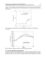
The next step is to record the readings and plot them on graph paper to develop a curve (Fig. 12). By comparing
the curves resulting from end-quench tests of different grades of steel (Fig. 13), relative hardenability can be
established. Steels with higher hardenability will be harder at a given distance from the quenched end of the
specimen than steels with lower hardenability. Thus, the flatter the curve is, the greater the hardenability will
be. On the end-quench curves, hardness usually is not measured beyond approximately 50 mm (2 in.) because
hardness measurements beyond this distance are seldom of any significance. At approximately 50 mm (2 in.)
from the quenched end, the effect of water on the quenched end has deteriorated, and the effect of cooling from
the surrounding air has become significant. An absolutely flat curve demonstrates conditions of very high
hardenability, which characterize an air-hardening steel, such as some highly alloyed steels.

Fig. 12 Method of developing end-quench curve by plotting hardness versus distance
from quenched end. Hardness plotted every 6.4 mm ( in.), although Rockwell C readings
were taken in increments of 1.59 mm ( in.), as shown on top of illustration.

Fig. 13 Plot of end-quench test results for five different steels
Additional information about Jominy end-quench hardenability is provided in the article “Quantitative

Prediction of Transformation Hardening in Steels” in Heat Treating, Volume 4 of ASM Handbook.


Introduction to Adhesion, Friction, and Wear
Testing
Peter J. Blau, Oak Ridge National Laboratory

Introduction
THE SURFACES OF SOLIDS play many different and important roles in technology. Their functions range
from imparting a pleasing appearance to protecting the underlying material from wear and corrosion, and from
bearing contact loads to serving as the substrates for coatings. The properties of free surfaces differ from those
of bulk materials. A variety of specialized testing methods, therefore, have been developed specifically for
characterizing the mechanical behavior of surfaces and the treatments and coatings applied to them.
In some engineering applications, like the bonding or fastening of parts, surfaces are placed in intimate contact
with the intention that they will not move relative to one another. In other cases, as in bearings, gears, brakes,
and rotating face seals, adjacent surfaces are intended to move relative to one another in a smooth and stable
fashion, while at the same time supporting a normal load. Sometimes, as in the attachment of protective
coatings to a surface, strong adhesion is desirable, but in other instances, as in the seizure and galling of sliding
bearings, strong adhesion is not desirable. Likewise, low friction might be desirable for a face seal but
undesirable for a brake pad. A high rate of abrasive wear for a paper mill slitter-knife blade is to be avoided, yet
the high abrasive wear rate associated with grinding prepares the surfaces of castings for mating with other
parts. Consequently, adhesion, friction, and wear are neither inherently good nor bad. Rather, they are
important to both the cosmetic and engineering functions of parts and must, therefore, be measured and
controlled.
Under some conditions, adhesion, friction, and wear are directly related, but under other conditions they are
not. For example, when clean metals rub against one another, adhesion can occur, raising the friction and
promoting the deformation and fracture of the softer material. The more extensive these processes are, the more
the wear. By contrast, there are cases in which the sliding friction of an interface can be relatively high (disc
brake pads against rotors), but the wear of the materials involved is relatively low. While appearing contrary to
intuition, the high-friction/low-wear situation becomes understandable when friction is viewed as the energy

available to do work on a material, and wear is but one of the possible ways in which a system can dissipate
that energy—conversion into heat being another. Thus, two sliding couples can possess nearly the same friction
coefficients but greatly different wear rates.
In this Section, tests designed specifically to evaluate the adhesion, friction, and wear behavior of various
material systems are described. Included within the wear category are other forms of surface damage, like
galling and scuffing. Unlike other mechanical properties, such as the elastic constants or shear strength,
properties of adhesion, friction, and wear depend strongly upon the surface conditions of the solid and not
exclusively upon its bulk structure. The selection of appropriate test methods to meet engineering requirements
for adhesion, friction, and wear, therefore, is somewhat complicated. Each functional requirement must be
analyzed on a case-by-case basis, and no one test is universally the best for measuring either adhesion, friction,
or wear.

Introduction to Adhesion, Friction, and Wear Testing
Peter J. Blau, Oak Ridge National Laboratory

Adhesion Testing
The article “Adhesion Testing” in this Section describes many different techniques and test methods that have
been devised for measuring the adhesion between solids. There is little standardization in this field, although
some investigators tend to favor one method over another. Most adhesion test methods are designed to assess
the ability of two materials to remain connected to one another despite the application of external or internal
body forces in various directions with respect to the interface. For example, different types of adhesion tests
have been designed to measure resistance to peeling, shearing, and delamination. In a few instances, adhesion
tests are used in the study of frictional phenomena that occur at a fine scale between protuberances on mating
surfaces. The article on adhesion testing contains a more complete discussion of these test methods and a
bibliography.

Introduction to Adhesion, Friction, and Wear Testing
Peter J. Blau, Oak Ridge National Laboratory

Friction Testing

Friction and wear are not basic properties of materials but rather represent the response of a material pair in a
certain environment to imposed forces, which tend to produce relative motion between the paired materials.
Friction and wear behavior is, therefore, subject to the considerations of testing geometry, the characteristics of
the relative motion, the contact pressure between the surfaces, the temperature, the stiffness and vibrational
properties of the supporting structures, the presence or absence of third bodies, the duration of contact, and the
chemistry of the environment in and around the interface. Tables of friction coefficients should not be trusted to
provide applicable numerical values unless the conditions used to develop the data closely mimic those of the
application for which the data are intended. Since frictional interactions occur under a wide variety of contact
conditions and size scales, selecting test methods for screening materials or lubricants for frictional behavior
should be done with care.
The article “Testing Methods for Solid Friction” describes a variety of methods that have proven useful in
measuring friction coefficients, both under static and kinetic conditions. Since frictional response is sometimes
sensitive to the preparation and cleaning of surfaces, these factors should be addressed when developing friction
testing procedures. Other testing variables, some of them rather subtle (like the fixture stiffness or thermal
conductivity), can affect friction test results in some cases. Frictional transitions, like running-in, are common
in engineering systems (Ref 1), so they should be considered when deciding on the type of data collection
method.
Standard test methods, like those produced by ASTM, can be useful not only as guides to friction testing
procedures but also as a source of information on which test variables should be controlled. Published
standards, like friction test methods in general, do not address all possible needs for friction measurement, and
thus, the engineer might need to devise his or her own tests to fit the situation.
Reference cited in this section
1. P.J. Blau, Friction Science and Technology, Marcel Dekker, Inc., 1996

Introduction to Adhesion, Friction, and Wear Testing
Peter J. Blau, Oak Ridge National Laboratory

Scratch Testing
Scratch tests are used for two main purposes:(a) to measure the adhesion of a coating or film to a surface, or (b)
to measure the resistance of a surface to damage from a harder opposing body. Scratch testing methods for the

former purpose are described in the article “Adhesion Testing.” Scratch tests used for the latter purpose are
described in the article “Scratch Testing” in this Volume. The use of scratch tests has a relatively long history,
having been introduced by the German mineralogist Friedrich Mohs in 1822 for identifying different mineral
species. The ability of a mineral to scratch or be scratched by another mineral is an important clue to its
identification, and use of the Mohs test persists to this day.
During recent years, scratch tests have been instrumented using force and acoustic emission sensors to provide
additional information for materials and coatings characterization. Diamond is the material of choice for most
scratch testing indenters, but diamond is not the only material used in scratch tests. Hardened steel files, for
example, are used for scratch testing under certain circumstances. New testing parameters, such as the critical
load for coating failure and the scratching coefficient (i.e., the normal force divided by the tangential force that
resists scratching), have been introduced to measure other surface properties. Scratch tests can be useful for
obtaining numerical rankings of the resistance of a material to single-point abrasion and for assessing the
mechanisms of material removal under abrasive conditions.

Introduction to Adhesion, Friction, and Wear Testing
Peter J. Blau, Oak Ridge National Laboratory

Testing for Wear and Surface Damage of Various Kinds
Because wear and surface damage take on many different forms, several articles on wear and surface damage
testing have been included in this Volume. Wear is a form of mechanically induced surface damage that results
in the progressive removal of material from a surface. Galling, chipping, or scratching can occur with one
contact event, and not being progressive, these phenomena are not strictly forms of wear. However, they still
fall under the category of surface damage. Because a great many types of surface damage occur in machinery,
different types of tests have been developed. The chapters in this Section describe quite a few of them, but it is
possible that a specialized method must be developed to effect a simulation of specific conditions or to isolate a
certain form of wear for detailed study.
Selection of the right type of test becomes critically important in order to achieve engineering relevance. In
fact, materials and surface treatments can rank in opposite order when tested for resistance to different forms of
wear (Ref 2). More than one type of wear can attack the same part, like both sliding and impact wear in printing
presses, and both erosive and abrasive wear on plastic extrusion machine screws. Sometimes wear can operate

in the presence of corrosive or chemically active environments, and synergistic chemomechanical effects are
possible. The selection of an appropriate wear testing method begins with an assessment of the type of wear
involved as well as the mechanical conditions and the environment that produced it.
Having a structured classification of wear types can make test selection easier. Different classification schemes
for wear have been developed because those who developed them have come from different backgrounds with
different experiences with wear. No one scheme is universally accepted, but most systems have similar features.
For example, mechanical wear can be classified by the type of relative motion: (a) tangential motion (sliding),
(b) impact, and (c) rolling (Ref 3). An abbreviated summary of the common wear and surface damage types,
categorized in this way, is given in Table 1. Formal definitions for the important types of wear are provided in
the ASM Handbook, Vol 18, Friction, Lubrication and Wear Technology (Ref 4). That Volume also contains
reviews of each major form of wear and comprehensive discussions of wear mechanisms, the wear of different
types of materials, and application-specific methods for wear control.




Table 1 Common types of wear and mechanical surface damage
Category Characteristics
Sliding wear Tangential motion and traction between surfaces
2 body abrasive wear Wear by fixed hard particles moving along a surface
3 body abrasive wear Wear by hard particles passing between opposing bodies
Adhesive wear Wear arising from the localized adhesion of one surface to another, which results in
plastic deformation and fracture with the transfer of detached material to the opposing
surface
Fretting wear Wear arising from short-amplitude oscillations or tangential contact vibrations
Fatigue wear Wear involving the nucleation and propagation of surface and/or subsurface cracks
under cyclic tangential forces arising from sliding contact
Polishing wear Fine-scale wear by the action of hard particles, chemomechanical processes, or both
Impact wear Normal forces acting cyclically on surfaces
Single-body impact

wear
Wear from the repeated impact of a second body
Multibody impact
wear
Wear from the repeated impact of particles, bubbles, droplets, or energy discharges.
Examples include particle impingement erosion, cavitation erosion (wear by
imploding bubbles), slurry erosion, and spark erosion.
Rolling contact wear Wear from the accumulation of surface damage during the cyclic stressing of one
body rolling over or along another
Surface damage other
than wear (examples)
Loss or displacement of material from a surface owing to mechanical contact in some
form
Chipping Removal of material from a surface, generally involving brittle crack propagation and
the production of shell-like features. Chipping commonly occurs at sharp corners or
edges of brittle contact surfaces.
Scuffing Plastic deformation of surface material by rubbing, which generally produces a
smooth appearance and is often localized in certain areas of the surface. Scuffing is
sometimes referred to as incipient galling.
Scratching Production of one or more shallow grooves in a surface by a hard counter body
moving tangentially along the surface
Galling A severe form of surface material displacement involving plastic deformation and the
loss of fit between counter surfaces
Gouging A severe form of localized plastic deformation in which relatively deep, localized
troughs are produced
Scoring Production of one or more deep scratches in a body generally involving plowing by a
hard particle or protuberance on an opposing body
False Brinelling Production of clusters of craters similar in appearance to hardness indentations with a
spherical indenter
Frosting The production of a dull appearance, typically on a bearing surface, due to a random

pattern of fine scratches or gouges
The descriptions given in the “Characteristics” column of Table 1 suggest that the use of wear terminology is
not without ambiguities. It is therefore important, when discussing or reporting on wear problems, to describe
the phenomena sufficiently well so that terminology ambiguities are avoided. Wear problems can be further
complicated by environmental interactions, such as oxidation or other surface chemical reactions, which occur
along with wear. In fact, some wear classification schemes list oxidational or chemical wear as major forms of
wear. Tests for most of the important forms of wear listed in Table 1 are described in this section. Sources for
information regarding impact wear, polishing wear, and other types not covered here are listed in the
bibliography.
Abrasive wear is one of the most economically important types of wear. The cost of damaged equipment, down
time, and materials loss attributable to abrasive wear in the mining and agriculture industries alone is
staggering. Several types of two-body and three-body abrasive wear tests are described. As with other types of
wear, more than one kind of test can be needed to establish the suitability of a given material, coating, or
surface treatment for complex abrasive environments.
Erosive wear, as indicated in Table 1, can involve removal of material by impinging solids, liquids, liquid-
entrained or gas-entrained solids, bubbles (cavitation erosion), or sparks. Like abrasive wear, erosive wear is a
costly form of wear in industry. It attacks piping, pumping equipment, turbomachinery, and conveyor systems.
Loose particles from erosive wear can also travel to other parts of a machine, creating secondary damage and
loss of function. The variables associated with different types of erosive wear tests commonly include
impingement angle, impingement velocity, screening by rebounding particles, and the shapes and sizes of the
erodent particles.
Sliding contact, like galling or scuffing, can produce surface damage with only one contact event, or it can be a
progressive form of wear like fretting or other repetitive contact types of wear. The article “Testing for Sliding
Contact Damage” in this Section describes several forms of sliding contact damage and the methods commonly
used to evaluate the resistance of materials to these damages.
Just as machines and their parts exist in a spectrum of sizes, friction and wear phenomena can also occur in
various size scales. Obviously, the fine-scale interfacial contact processes involved in nanoscale coatings on
hard disks require a different testing approach than the macroscale wear that occurs on the digger teeth of
mining equipment and on the bows of icebreakers. Therefore, not only are there different types of wear, like
abrasive wear, erosive wear, and so on, but there are also different size-scales of wear phenomena.

References cited in this section
2. H. Czichos, Tribology: A Systems Approach, Elsevier, Amsterdam, Netherlands, 1978, p 322–325
3. P.J. Blau, Wear Testing, Metals Handbook Desk Edition, ASM International, 1998, p 1342–1347
4. P.J. Blau, Glossary, Friction, Lubrication, and Wear Technology, Vol 18, ASM Handbook, ASM
International, 1992, p 1–21

Introduction to Adhesion, Friction, and Wear Testing
Peter J. Blau, Oak Ridge National Laboratory

Testing for Wear and Surface Damage of Various Kinds
Because wear and surface damage take on many different forms, several articles on wear and surface damage
testing have been included in this Volume. Wear is a form of mechanically induced surface damage that results
in the progressive removal of material from a surface. Galling, chipping, or scratching can occur with one
contact event, and not being progressive, these phenomena are not strictly forms of wear. However, they still
fall under the category of surface damage. Because a great many types of surface damage occur in machinery,
different types of tests have been developed. The chapters in this Section describe quite a few of them, but it is
possible that a specialized method must be developed to effect a simulation of specific conditions or to isolate a
certain form of wear for detailed study.
Selection of the right type of test becomes critically important in order to achieve engineering relevance. In
fact, materials and surface treatments can rank in opposite order when tested for resistance to different forms of
wear (Ref 2). More than one type of wear can attack the same part, like both sliding and impact wear in printing
presses, and both erosive and abrasive wear on plastic extrusion machine screws. Sometimes wear can operate
in the presence of corrosive or chemically active environments, and synergistic chemomechanical effects are
possible. The selection of an appropriate wear testing method begins with an assessment of the type of wear
involved as well as the mechanical conditions and the environment that produced it.
Having a structured classification of wear types can make test selection easier. Different classification schemes
for wear have been developed because those who developed them have come from different backgrounds with
different experiences with wear. No one scheme is universally accepted, but most systems have similar features.
For example, mechanical wear can be classified by the type of relative motion: (a) tangential motion (sliding),
(b) impact, and (c) rolling (Ref 3). An abbreviated summary of the common wear and surface damage types,

categorized in this way, is given in Table 1. Formal definitions for the important types of wear are provided in
the ASM Handbook, Vol 18, Friction, Lubrication and Wear Technology (Ref 4). That Volume also contains
reviews of each major form of wear and comprehensive discussions of wear mechanisms, the wear of different
types of materials, and application-specific methods for wear control.
Table 1 Common types of wear and mechanical surface damage
Category
Characteristics
Sliding wear
Tangential motion and traction between surfaces
2 body abrasive
wear
Wear by fixed hard particles moving along a surface
3 body abrasive
wear
Wear by hard particles passing between opposing bodies
Adhesive wear
Wear arising from the localized adhesion of one surface to another, which results
in plastic deformation and fracture with the transfer of detached material to the
opposing surface
Fretting wear
Wear arising from short-amplitude oscillations or tangential contact vibrations
Fatigue wear
Wear involving the nucleation and propagation of surface and/or subsurface
cracks under cyclic tangential forces arising from sliding contact
Polishing wear
Fine-scale wear by the action of hard particles, chemomechanical processes, or
both
Impact wear
Normal forces acting cyclically on surfaces
Single-body impact

wear
Wear from the repeated impact of a second body
Multibody impact
wear
Wear from the repeated impact of particles, bubbles, droplets, or energy
discharges. Examples include particle impingement erosion, cavitation erosion
(wear by imploding bubbles), slurry erosion, and spark erosion.
Rolling contact wear
Wear from the accumulation of surface damage during the cyclic stressing of one
body rolling over or along another
Surface damage other
than wear (examples)
Loss or displacement of material from a surface owing to mechanical contact in
some form
Chipping
Removal of material from a surface, generally involving brittle crack propagation
and the production of shell-like features. Chipping commonly occurs at sharp
corners or edges of brittle contact surfaces.
Scuffing
Plastic deformation of surface material by rubbing, which generally produces a
smooth appearance and is often localized in certain areas of the surface. Scuffing
is sometimes referred to as incipient galling.
Scratching
Production of one or more shallow grooves in a surface by a hard counter body
moving tangentially along the surface
Galling
A severe form of surface material displacement involving plastic deformation and
the loss of fit between counter surfaces
Gouging
A severe form of localized plastic deformation in which relatively deep, localized

troughs are produced
Scoring
Production of one or more deep scratches in a body generally involving plowing
by a hard particle or protuberance on an opposing body
False Brinelling
Production of clusters of craters similar in appearance to hardness indentations
with a spherical indenter
Frosting The production of a dull appearance, typically on a bearing surface, due to a
random pattern of fine scratches or gouges
The descriptions given in the “Characteristics” column of Table 1 suggest that the use of wear terminology is
not without ambiguities. It is therefore important, when discussing or reporting on wear problems, to describe
the phenomena sufficiently well so that terminology ambiguities are avoided. Wear problems can be further
complicated by environmental interactions, such as oxidation or other surface chemical reactions, which occur
along with wear. In fact, some wear classification schemes list oxidational or chemical wear as major forms of
wear. Tests for most of the important forms of wear listed in Table 1 are described in this section. Sources for
information regarding impact wear, polishing wear, and other types not covered here are listed in the
bibliography.
Abrasive wear is one of the most economically important types of wear. The cost of damaged equipment, down
time, and materials loss attributable to abrasive wear in the mining and agriculture industries alone is
staggering. Several types of two-body and three-body abrasive wear tests are described. As with other types of
wear, more than one kind of test can be needed to establish the suitability of a given material, coating, or
surface treatment for complex abrasive environments.
Erosive wear, as indicated in Table 1, can involve removal of material by impinging solids, liquids, liquid-
entrained or gas-entrained solids, bubbles (cavitation erosion), or sparks. Like abrasive wear, erosive wear is a
costly form of wear in industry. It attacks piping, pumping equipment, turbomachinery, and conveyor systems.
Loose particles from erosive wear can also travel to other parts of a machine, creating secondary damage and
loss of function. The variables associated with different types of erosive wear tests commonly include
impingement angle, impingement velocity, screening by rebounding particles, and the shapes and sizes of the
erodent particles.
Sliding contact, like galling or scuffing, can produce surface damage with only one contact event, or it can be a

progressive form of wear like fretting or other repetitive contact types of wear. The article “Testing for Sliding
Contact Damage” in this Section describes several forms of sliding contact damage and the methods commonly
used to evaluate the resistance of materials to these damages.
Just as machines and their parts exist in a spectrum of sizes, friction and wear phenomena can also occur in
various size scales. Obviously, the fine-scale interfacial contact processes involved in nanoscale coatings on
hard disks require a different testing approach than the macroscale wear that occurs on the digger teeth of
mining equipment and on the bows of icebreakers. Therefore, not only are there different types of wear, like
abrasive wear, erosive wear, and so on, but there are also different size-scales of wear phenomena.
References cited in this section
2. H. Czichos, Tribology: A Systems Approach, Elsevier, Amsterdam, Netherlands, 1978, p 322–325
3. P.J. Blau, Wear Testing, Metals Handbook Desk Edition, ASM International, 1998, p 1342–1347
4. P.J. Blau, Glossary, Friction, Lubrication, and Wear Technology, Vol 18, ASM Handbook, ASM
International, 1992, p 1–21

Introduction to Adhesion, Friction, and Wear Testing
Peter J. Blau, Oak Ridge National Laboratory

Adhesion, Friction, and Wear Testing Devices
Literally hundreds of devices for measuring adhesion, friction, and wear have been developed. Some of these
are commercially manufactured but most of them probably have been custom-designed for specific purposes.
This situation makes it difficult to compare the results from one study with those of another study unless the
appropriate correlation has been established. There is no simple answer to the problems arising from the
proliferation of different testing machines for adhesion, friction, and wear. The use of established voluntary
standards can help, but only if the standard applies directly to the problem of current concern. In the absence of
widespread, commonly used test methods, it is necessary to analyze the applied conditions associated with each
set of results carefully to determine the extent to which they can be compared to other work.
As with mechanical testing in general, commercial adhesion, friction, and wear testing machines are becoming
increasingly computer automated. While automation has obvious advantages, it also necessitates conscientious
calibration to ensure that the sensors and control mechanisms provide accurate readings to the computer.
In adhesion, friction, and wear testing, as in other forms of mechanical testing, the four most important

requirements are (a) understanding the characteristics of the test method being applied, (b) expecting differing
degrees of repeatability from different material types, (c) selecting the right testing tool for the job, and (d)
coupling measurements with physical observations of contact surfaces to ascertain the causes for the measured
behavior.

Introduction to Adhesion, Friction, and Wear Testing
Peter J. Blau, Oak Ridge National Laboratory

References
1. P.J. Blau, Friction Science and Technology, Marcel Dekker, Inc., 1996
2. H. Czichos, Tribology: A Systems Approach, Elsevier, Amsterdam, Netherlands, 1978, p 322–325
3. P.J. Blau, Wear Testing, Metals Handbook Desk Edition, ASM International, 1998, p 1342–1347
4. P.J. Blau, Glossary, Friction, Lubrication, and Wear Technology, Vol 18, ASM Handbook, ASM
International, 1992, p 1–21
5. D.F. Moore, Principles and Applications of Tribology, Pergamon Press, Oxford, 1975, p 62–85

Introduction to Adhesion, Friction, and Wear Testing
Peter J. Blau, Oak Ridge National Laboratory

Selected References
• B. Bhushan and B.K. Gupta, Handbook of Tribology, McGraw-Hill, 1991
• Friction and Wear Testing Source Book, ASM International, 1997
• Friction, Lubrication, and Wear Technology, Vol 18, ASM Handbook, ASM International, 1992
• Metals Handbook Desk Edition, 2nd ed., ASM International, 1998
• R.G. Bayer, Mechanical Wear Prediction and Prevention, Marcel Dekker, Inc., 1995
• Special Technical Publications, ASTM
• W.A. Glaeser, Characterization of Tribological Materials, Butterworth-Heinemann Ltd., Boston, 1993
• Wear Control Handbook, M.B. Peterson and W.O. Winer, Ed., American Society of Mechanical
Engineers, 1980

Adhesion Testing

Introduction
ADHESION refers to the interfacial bond strength between two materials in close proximity with one another.
Adhesive bond strength can be described in several ways, depending on the nature of the interface. In physical
chemistry, for example, adhesion is a fundamental term that refers to the attractive force between a solid
surface and a second phase in either liquid or solid form. In this context, adhesion is a manifestation of the
innate interatomic and intermolecular bonds that occur between the surfaces of two materials.
Other meanings of adhesion also arise in different disciplines related to mechanical engineering and the
evaluation of coatings and films. In railway engineering, for example, adhesion often means friction (Ref 1) or
the sliding resistance between two materials. In this context, the term adhesion refers to mechanical adhesion,
which is defined as the adhesion produced by the interlocking of protuberances on the surfaces in an interface
(Ref 1).
Adhesion also has important practical meaning in the evaluation of coatings, adhesives, and composite
materials. Thin films (<1 μm, or 0.04 mil), thick films (>1 μm), and bulk coatings (>25 μm, or 98 mils) all
depend on adhesion, which can be evaluated and measured in a variety of ways, depending on the product
configuration and application requirements. Therefore, it is not surprising that many methods are used to
measure adhesion for films, coatings, and adhesive-bonded joints. Indeed, there are so many variations on
adhesion measurements in coatings, surface films, and adhesives (Ref 2, 3, 4, 5, 6) that it would be impossible
to describe them fully here.
Therefore, the purpose of this article is to describe briefly common adhesion measurement techniques for the
three basic types of adhesion outlined by Mittal (Ref 2 and 6):
1. Fundamental (or basic) adhesion
2. Thermodynamic adhesion
3. Practical adhesion
Common measurement methods for each type of adhesion are briefly discussed, with the main focus on
practical adhesion testing of coatings and thin films. However, to illustrate the use of adhesion testing in
materials research, this article also includes a section on the use of adhesion tests in the evaluation of stress-
corrosion cracking (SCC) within bimaterial interfaces.
References cited in this section

1. P.J. Blau, Glossary of Terms, Friction, Lubrication, and Wear Technology, Vol 18, ASM Handbook,
ASM International, 1992
2. K.L. Mittal, Ed., Adhesion Measurements of Films and Coatings, VSP, 1995
3. K.L. Mittal, Ed., Adhesive Joints, Plenum Press, 1984
4. G.L. Schneberger, Ed., Adhesives in Manufacturing, Marcel Dekker, 1983
5. G.P. Anderson, S.J. Bennett, and K.L. DeVries, Analysis and Testing of Adhesive Bonds, Academic
Press, 1977
6. K.L. Mittal, Ed., Adhesion Measurement of Thin Films, Thick Films and Bulk Coatings, STP 640,
ASTM, 1978

Adhesion Testing

Fundamental Adhesion
Fundamental adhesion refers to the basic intermolecular forces that occur whenever two materials are in close
proximity. These intermolecular forces that act between the surfaces of bodies are called surface forces (Ref 7,
8), and adhesion is one manifestation of the existence of surface forces.
Surface Forces
Fundamental adhesion arises from innate surface forces, which have their origins in well-understood
interatomic and intermolecular forces (Ref 7). Such forces are always present, and they can be described by the
summation of individual bond strengths over a unit area or by the energy required to break chemical bonds at
the weakest plane or loci of points within an interface (Ref 2).
It is sometimes convenient to classify surface forces as either short-range or long-range surface forces. Short-
range surface forces are those that act between atoms and molecules that are essentially in contact, say within
0.1 or 0.2 nm of each other. Examples of this are covalent and hydrogen bonding, as well as Born repulsions.
Long-range surface forces act between surfaces that are farther apart, which in this context means on the order
of a few nanometers. Examples of long-range surface forces include van der Waals and electrostatic forces.
However, some short-range surface forces also produce effects over a longer range. An example of this is steric
repulsion. In this case, surfactant molecules adsorbed on a solid surface (via short-range bonding) can prevent a
second surface from approaching the first. Boundary lubricants operate in this way to keep solid surfaces
separated.

In general, short-range forces are stronger than long-range forces and make the most important contributions to
adhesion. Unfortunately, long-range forces are easier to both measure and model. Therefore, knowledge of
surface forces, from both a theoretical and experimental standpoint, is much sounder for long-range effects.
This is why an understanding of fundamental adhesion based on short-range surfaces forces has proven to be
difficult (Ref 9).
Measurement of Surface Forces
“Long-range” surface forces act over surface separations from 1 to 100 nm and cause forces levels in the range
of about 10
-7
to 10
-4
N. Measuring these forces is not a trivial matter. The magnitude of the forces increases
with surface area (or, as shown below, with the radius of curved surfaces). Thus, in order to have measurable
forces, it is desirable to have extended areas of surface. At the same time, to make sensible measurements of
surface separation on a nanometer scale, it is necessary for the surfaces to be extremely smooth. A method of
detecting small forces is required, as are methods of controlling and measuring very small surface separations.
Although surface force measurements have been made for several decades, the inherent difficulties of surface
preparation and cleanliness limited the number of materials studied and the amount of data to a small level,
until about 1970. The most popular technique has been the crossed-cylinder apparatus devised by Tabor (Ref
10) and further developed by Israelachvili (Ref 11). This technique uses a surface force apparatus (SFA), which
is commercially available. A review of the field up until 1982 is also provided in Ref 12.
The SFA consists of a closed stainless steel chamber designed to enclose a variety of liquid or vapor media and
is usually operated at ambient temperature and pressure. Force is measured between two cylindrical surfaces,
with the axes of the cylinders at right angles to each other (Fig. 1). The reason for choosing this geometry is for
purposes of practicality. If two planar surfaces were to be used (as one might have supposed), then there would
be extreme difficulties in forming surfaces of sufficient flatness, mounting them exactly parallel, maintaining
parallelism while moving the surfaces together or apart, and avoiding edge effects, all while working on a
nanometer scale. As shown in the next section, “The Derjaguin Approximation,” it turns out that there is no
difficulty interpreting the forces measured in this odd geometry because there is a simple relationship between
the force measured between crossed cylinders and the energy of interaction between flat surfaces.

Fig. 1 Surface force apparatus, in which two thin solid substrates are mounted as cross cylinders, with
one of them supported by a cantilever spring whose deflection measures the force. An optical
interferometric technique is used to measure the distance between the surfaces.
In order to measure surface separation, the SFA employs an optical interference technique (Ref 11, 13, 14).
Under optimal conditions, this gives a resolution of 0.1 nm or better. Of course, one drawback is that it places a
limitation on the solid materials that can be investigated; namely, that at least one of the pair whose surfaces
approach contact must be transparent and rather thin (ideally, a few mm). Most of the measurements made with
this apparatus have been made with thin foils of mica bent around and glued to cylindrical glass lenses.
To implement the optical method, a 95% reflecting silver layer is coated on the outer (that is, remote) surface of
each solid substrate. Collimated white light is shone through the two substrates and whatever medium separates
them (Fig. 1). Multiple-beam interference between the two silver layers selects only certain wavelengths of
light, which are passed by the interferometer. All other wavelengths interfere destructively and are not
transmitted. The transmitted light is collected and directed to a grating spectrometer, which spreads it according
to wavelength, so that discrete wavelengths appear at the exit port of the spectrometer as spatially separated
fringes of equal chromatic order.
The wavelengths depend on the thicknesses and refractive indices of the materials that are included in the
interferometer: usually, the two transparent substrates and whatever fluid medium is between them.
Measurement and analysis of the wavelengths allow computation of these thicknesses (Ref 13, 14). Because the
two solids are of fixed thickness, those values can be subtracted from the total to give the thickness of the
intervening medium, that is, the separation, D, between the inner (adjacent) surfaces of the solids at their closest
point of approach.
The surface force that one solid substrate exerts on the others is measured by a simple spring-deflection
method. One solid is mounted on a cantilever spring, the remote end of which is moved up or down using a
three-stage drive mechanism. The first stage is a micrometer that allows coarse positioning of the surfaces from
a separation of a few mm to a few μm. The second stage is a micrometer that acts through a differential spring
mechanism, which reduces the motion a thousand-fold, allowing positioning to approximately 1 nm. Finally,
voltage applied to a piezoelectric tube expander gives positioning to a fraction of 1 nm.
After calibrating the drive mechanisms, it is straightforward to monitor any differences between a movement of
the remote end of the spring and the distance moved by the end that bears one of the solids. This difference

corresponds to a deflection of the spring. Multiplying it by the spring stiffness (typically 100 N/m, or 7 lbf/ft)
gives the increment in force resulting from the movement. Because both the calibration and the movement of
the solid are measured with a resolution of ~0.1 nm, it is possible to measure very small force changes (10
-7
to
10
-8
N) using this technique.
The Derjaguin Approximation. The force, F
c
, between two gently curved surfaces is proportional to the
interaction energy per unit area, E
f
, between two flat ones at the same separation. This relationship, known as
the Derjaguin approximation, allows straightforward interpretations to be made of surface force measurements
between crossed cylinders (or between one sphere and another or between a sphere and a flat plate). It is also
helpful in certain adhesion measurements, as described below.
The Derjaguin approximation is derived (see Ref 7, for example) by considering the force between each
element of one curved surface and each element of the other, and then integrating over the two surfaces to
obtain the total force. As long as the radius of curvature is much larger than the range of the surface force, this
is approximately equivalent to integrating the force per unit area, F
f
, between flat surfaces, from the minimum
separation of the curved surfaces, D, to an effectively infinite upper limit, with some geometrical factors to
account for the shape of the surfaces. The integral simply gives the interaction energy between flats, E
f
(D),
which is the work done against the surface forces in moving the flat surfaces from infinity to D. For two
spheres of radius R
1

and R
2
, the geometrical factor is a constant, giving:
F
c
(D) = 2π R E
f
(D)


where 1/R = 1/R
1
+ 1/R
2
. It can be shown that the geometry of crossed cylinders of equal radii, R
c
, is equivalent
to a sphere of radius R
c
approaching a flat plate, or to two spheres of radius 2 R
c
approaching each other.
Substrate Materials. The original and still most common solid material used in surface force measurements is
mica, chosen because it satisfies the requirements (thin and transparent) of the optical interference technique
used in the SFA and because it is easy to prepare large areas of molecularly smooth surface by cleavage.
Experiments have been conducted on mica surfaces immersed in many different liquid and vapor environments
(Ref 8).
Recently, there has been some success in extending these measurements to a wider range of surfaces. One
approach is to coat mica surfaces by various techniques, including Langmuir-Blodgett deposition, surfactant or
polymer adsorption from solution, plasma modification, and evaporative coating of thin metal, carbon, and

metal-oxide films. An alternative approach is to find a means of preparing other transparent materials as
micron-thick foils with very smooth surfaces. This has been done for sapphire, silica, pyrex glass, and certain
polymers. It is reasonable to expect that the range of materials studied will continue to increase in the near
future.
Currently, the best way to prepare metal surfaces for SFA appears to be thin-film evaporation onto mica or
another smooth substrate. Because the optical technique requires some light to pass through the two films, their
thicknesses cannot be more than a few tens of nanometers. It is possible to use the metal films themselves as
one or both optical interferometer mirrors, but the fringes of equal chromatic order would disappear from the
visible spectrum if the two metal surfaces were brought closer together than about 1 μm (40 μin.). In that case,
an alternative method of measuring separation, such as capacitance, would be required.
Environments. Tests with the surface force apparatus can be conducted in many different liquids or vapors, as
long as they are compatible with the materials of the SFA system (namely, stainless steel, silica, Kel-F, and
Teflon). There is a provision to heat the chamber to around 100 °C (212 °F). Use of an appropriate heating
jacket could extend the temperature range from, perhaps, -50 to 150 °C (-60 to 300 °F). At about 150 °C (300
°F), the silver layers used for interferometer mirrors degrade. This limit might be raised by using other optical
coatings. The next limitation of the current design would be the maximum operating temperature of the Teflon
seals, which is 250 °C (480 °F). In principle, the same or comparable techniques could be extended to operate
at several hundred degrees, but in practice this would require a major redesign of the apparatus.
At present, the SFA is intended only to operate at or near ambient pressure. With some modifications to the
seals, it could be made to hold moderate vacuum, say 10
-4
Pa (10
-6
torr). A total redesign would be required to
build a device for making comparable measurements in ultrahigh vacuum (UHV) conditions.
Preparation of Surfaces and Fluids. Any solid to be investigated by the SFA method should be smooth,
compared to the range of forces under examination. Because the adhesion between surfaces is often dominated
by very short-range forces, atomically smooth surfaces would be required to make fundamental and
reproducible measurements of these. However, rough surfaces still adhere, and so measurements can be made
without insisting on atomic smoothness. The drawback, in that case, is that it would be more difficult to obtain

a straightforward interpretation of the results.
Because SFA measurements involve extremely small surface separations, there are stringent requirements for
cleanliness. One speck of dust in the wrong place can spoil the entire test. The relative importance of surface
cleanliness is again related to the range of force under investigation. For very short-range forces, even a