The Fast Fourier Transform

225
CHAPTER
12
The Fast Fourier Transform
There are several ways to calculate the Discrete Fourier Transform (DFT), such as solving
simultaneous linear equations or the correlation method described in Chapter 8. The Fast
Fourier Transform (FFT) is another method for calculating the DFT. While it produces the same
result as the other approaches, it is incredibly more efficient, often reducing the computation time
by hundreds. This is the same improvement as flying in a jet aircraft versus walking! If the
FFT were not available, many of the techniques described in this book would not be practical.
While the FFT only requires a few dozen lines of code, it is one of the most complicated
algorithms in DSP. But don't despair! You can easily use published FFT routines without fully
understanding the internal workings.
Real DFT Using the Complex DFT
J.W. Cooley and J.W. Tukey are given credit for bringing the FFT to the world
in their paper: "An algorithm for the machine calculation of complex Fourier
Series," Mathematics Computation, Vol. 19, 1965, pp 297-301. In retrospect,
others had discovered the technique many years before. For instance, the great
German mathematician Karl Friedrich Gauss (1777-1855) had used the method
more than a century earlier. This early work was largely forgotten because it
lacked the tool to make it practical: the digital computer. Cooley and Tukey
are honored because they discovered the FFT at the right time, the beginning
of the computer revolution.
The FFT is based on the complex DFT, a more sophisticated version of the real
DFT discussed in the last four chapters. These transforms are named for the
way each represents data, that is, using complex numbers or using real
numbers. The term complex does not mean that this representation is difficult
or complicated, but that a specific type of mathematics is used. Complex
mathematics often is difficult and complicated, but that isn't where the name
comes from. Chapter 29 discusses the complex DFT and provides the
background needed to understand the details of the FFT algorithm. The

The Scientist and Engineer's Guide to Digital Signal Processing226
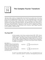
FIGURE 12-1
Comparing the real and complex DFTs. The real DFT takes an N point time domain signal and
creates two point frequency domain signals. The complex DFT takes two N point time
N/2 %1
domain signals and creates two N point frequency domain signals. The crosshatched regions shows
the values common to the two transforms.
Real DFT
Complex DFT
Time Domain
Time Domain
Frequency Domain
Frequency Domain
0 N-1
0 N-1
0 N-1
0 N/2
0 N/2
0
0
N-1
N-1
N/2
N/2
Real Part
Imaginary Part
Real Part
Imaginary Part
Real Part
Imaginary Part

Time Domain Signal
topic of this chapter is simpler: how to use the FFT to calculate the real DFT,
without drowning in a mire of advanced mathematics.
Since the FFT is an algorithm for calculating the complex DFT, it is
important to understand how to transfer real DFT data into and out of the
complex DFT format. Figure 12-1 compares how the real DFT and the
complex DFT store data. The real DFT transforms an N point time domain
signal into two point frequency domain signals. The time domainN/2 % 1
signal is called just that: the time domain signal. The two signals in the
frequency domain are called the real part and the imaginary part, holding
the amplitudes of the cosine waves and sine waves, respectively. This
should be very familiar from past chapters.
In comparison, the complex DFT transforms two N point time domain signals
into two N point frequency domain signals. The two time domain signals are
called the real part and the imaginary part, just as are the frequency domain
signals. In spite of their names, all of the values in these arrays are just
ordinary numbers. (If you are familiar with complex numbers: the j's are not
included in the array values; they are a part of the mathematics. Recall that the
operator, Im( ), returns a real number).
Chapter 12- The Fast Fourier Transform 227
6000 'NEGATIVE FREQUENCY GENERATION
6010 'This subroutine creates the complex frequency domain from the real frequency domain.
6020 'Upon entry to this subroutine, N% contains the number of points in the signals, and
6030 'REX[ ] and IMX[ ] contain the real frequency domain in samples 0 to N%/2.
6040 'On return, REX[ ] and IMX[ ] contain the complex frequency domain in samples 0 to N%-1.
6050 '
6060 FOR K% = (N%/2+1) TO (N%-1)
6070 REX[K%] = REX[N%-K%]
6080 IMX[K%] = -IMX[N%-K%]
6090 NEXT K%

6100 '
6110 RETURN
TABLE 12-1
Suppose you have an N point signal, and need to calculate the real DFT by
means of the Complex DFT (such as by using the FFT algorithm). First, move
the N point signal into the real part of the complex DFT's time domain, and
then set all of the samples in the imaginary part to zero. Calculation of the
complex DFT results in a real and an imaginary signal in the frequency
domain, each composed of N points. Samples 0 through N/2 of these signals
correspond to the real DFT's spectrum.
As discussed in Chapter 10, the DFT's frequency domain is periodic when the
negative frequencies are included (see Fig. 10-9). The choice of a single
period is arbitrary; it can be chosen between -1.0 and 0, -0.5 and 0.5, 0 and
1.0, or any other one unit interval referenced to the sampling rate. The
complex DFT's frequency spectrum includes the negative frequencies in the 0
to 1.0 arrangement. In other words, one full period stretches from sample 0 to
sample , corresponding with 0 to 1.0 times the sampling rate. The positiveN&1
frequencies sit between sample 0 and , corresponding with 0 to 0.5. TheN/2
other samples, between and , contain the negative frequencyN/2 %1 N&1
values (which are usually ignored).
Calculating a real Inverse DFT using a complex Inverse DFT is slightly
harder. This is because you need to insure that the negative frequencies are
loaded in the proper format. Remember, points 0 through in theN/2
complex DFT are the same as in the real DFT, for both the real and the
imaginary parts. For the real part, point is the same as pointN/2 %1
, point is the same as point , etc. This continues toN/2 &1 N/2 %2 N/2 &2
point being the same as point 1. The same basic pattern is used forN&1
the imaginary part, except the sign is changed. That is, point is theN/2 %1
negative of point , point is the negative of point , etc.N/2 &1 N/2 %2 N/2 &2
Notice that samples 0 and do not have a matching point in thisN/2

duplication scheme. Use Fig. 10-9 as a guide to understanding this
symmetry. In practice, you load the real DFT's frequency spectrum into
samples 0 to of the complex DFT's arrays, and then use a subroutine toN/2
generate the negative frequencies between samples and . TableN/2 %1 N&1
12-1 shows such a program. To check that the proper symmetry is present,
after taking the inverse FFT, look at the imaginary part of the time domain.
It will contain all zeros if everything is correct (except for a few parts-per-
million of noise, using single precision calculations).
The Scientist and Engineer's Guide to Digital Signal Processing228
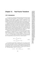
FIGURE 12-2
The FFT decomposition. An N point signal is decomposed into N signals each containing a single point.
Each stage uses an interlace decomposition, separating the even and odd numbered samples.
1 signal of
16 points
2 signals of
8 points
4 signals of
4 points
8 signals of
2 points
16 signals of
1 point
0 1 2 3 4 5 6 7 8 9 10 11 12 13 14 15
0 2 4 6 8 10 12 14 1 3 5 7 9 11 13 15
0 4 8 12 2 6 10 14 1 5 9 13 3 7 11 15
8 4 12 2 10 6 14 1 9 5 13 3 11 7 15
0
8 4 12 2 10 6 14 1 9 5 13 3 11 7 150
How the FFT works
The FFT is a complicated algorithm, and its details are usually left to those that

specialize in such things. This section describes the general operation of the
FFT, but skirts a key issue: the use of complex numbers. If you have a
background in complex mathematics, you can read between the lines to
understand the true nature of the algorithm. Don't worry if the details elude
you; few scientists and engineers that use the FFT could write the program
from scratch.
In complex notation, the time and frequency domains each contain one signal
made up of N complex points. Each of these complex points is composed of
two numbers, the real part and the imaginary part. For example, when we talk
about complex sample , it refers to the combination of andX[42] ReX[42]
. In other words, each complex variable holds two numbers. WhenImX[42]
two complex variables are multiplied, the four individual components must be
combined to form the two components of the product (such as in Eq. 9-1). The
following discussion on "How the FFT works" uses this jargon of complex
notation. That is, the singular terms: signal, point, sample, and value, refer
to the combination of the real part and the imaginary part.
The FFT operates by decomposing an N point time domain signal into N
time domain signals each composed of a single point. The second step is to
calculate the N frequency spectra corresponding to these N time domain
signals. Lastly, the N spectra are synthesized into a single frequency
spectrum.
Figure 12-2 shows an example of the time domain decomposition used in the
FFT. In this example, a 16 point signal is decomposed through four
Chapter 12- The Fast Fourier Transform 229
Sample numbers Sample numbers
in normal order after bit reversal
Decimal Binary Decimal Binary
0 0000 0 0000
1 0001 8 1000
2 0010 4 0100

3 0011 12 1100
4 0100 2 0010
5 0101 10 1010
6 0110 6 0100
7 0111 14 1110
8 1000 1 0001
9 1001 9 1001
10 1010 5 0101
11 1011 13 1101
12 1100 3 0011
13 1101 11 1011
14 1110 7 0111
15 1111 15 1111
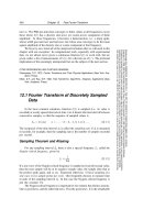
FIGURE 12-3
The FFT bit reversal sorting. The FFT time domain decomposition can be implemented by
sorting the samples according to bit reversed order.
separate stages. The first stage breaks the 16 point signal into two signals each
consisting of 8 points. The second stage decomposes the data into four signals
of 4 points. This pattern continues until there are N signals composed of a
single point. An interlaced decomposition is used each time a signal is
broken in two, that is, the signal is separated into its even and odd numbered
samples. The best way to understand this is by inspecting Fig. 12-2 until you
grasp the pattern. There are stages required in this decomposition, i.e.,Log
2
N
a 16 point signal (2
4
) requires 4 stages, a 512 point signal (2
7
) requires 7

stages, a 4096 point signal (2
12
) requires 12 stages, etc. Remember this value,
; it will be referenced many times in this chapter.Log
2
N
Now that you understand the structure of the decomposition, it can be greatly
simplified. The decomposition is nothing more than a reordering of the
samples in the signal. Figure 12-3 shows the rearrangement pattern required.
On the left, the sample numbers of the original signal are listed along with
their binary equivalents. On the right, the rearranged sample numbers are
listed, also along with their binary equivalents. The important idea is that the
binary numbers are the reversals of each other. For example, sample 3 (0011)
is exchanged with sample number 12 (1100). Likewise, sample number 14
(1110) is swapped with sample number 7 (0111), and so forth. The FFT time
domain decomposition is usually carried out by a bit reversal sorting
algorithm. This involves rearranging the order of the N time domain samples
by counting in binary with the bits flipped left-for-right (such as in the far right
column in Fig. 12-3).
The Scientist and Engineer's Guide to Digital Signal Processing230
a b c d
a
b
c d
0
0 0 0
A
B C
D
A B

C
D A B C D
e
f
g
h
e f
g
h
0
0
0 0
E
F G H
F G H E F G H
× sinusoid
Time Domain Frequency Domain
E
FIGURE 12-4
The FFT synthesis. When a time domain signal is diluted with zeros, the frequency domain is
duplicated. If the time domain signal is also shifted by one sample during the dilution, the spectrum
will additionally be multiplied by a sinusoid.
The next step in the FFT algorithm is to find the frequency spectra of the
1 point time domain signals. Nothing could be easier; the frequency
spectrum of a 1 point signal is equal to itself. This means that nothing is
required to do this step. Although there is no work involved, don't forget
that each of the 1 point signals is now a frequency spectrum, and not a time
domain signal.
The last step in the FFT is to combine the N frequency spectra in the exact
reverse order that the time domain decomposition took place. This is where the

algorithm gets messy. Unfortunately, the bit reversal shortcut is not
applicable, and we must go back one stage at a time. In the first stage, 16
frequency spectra (1 point each) are synthesized into 8 frequency spectra (2
points each). In the second stage, the 8 frequency spectra (2 points each) are
synthesized into 4 frequency spectra (4 points each), and so on. The last stage
results in the output of the FFT, a 16 point frequency spectrum.
Figure 12-4 shows how two frequency spectra, each composed of 4 points,
are combined into a single frequency spectrum of 8 points. This synthesis
must undo the interlaced decomposition done in the time domain. In other
words, the frequency domain operation must correspond to the time domain
procedure of combining two 4 point signals by interlacing. Consider two
time domain signals, abcd and efgh. An 8 point time domain signal can be
formed by two steps: dilute each 4 point signal with zeros to make it an
Chapter 12- The Fast Fourier Transform 231
++ + + + + + +
Eight Point Frequency Spectrum
Odd- Four Point
Frequency Spectrum
Even- Four Point
Frequency Spectrum
S
x
S
x
S
x
S
x
FIGURE 12-5
FFT synthesis flow diagram. This shows

the method of combining two 4 point
frequency spectra into a single 8 point
frequency spectrum. The ×S operation
means that the signal is multiplied by a
sinusoid with an appropriately selected
frequency.
2 point input
2 point output
S
x
FIGURE 12-6
The FFT butterfly. This is the basic
calculation element in the FFT, taking
two complex points and converting
them into two other complex points.
8 point signal, and then add the signals together. That is, abcd becomes
a0b0c0d0, and efgh becomes 0e0f0g0h. Adding these two 8 point signals
produces aebfcgdh. As shown in Fig. 12-4, diluting the time domain with zeros
corresponds to a duplication of the frequency spectrum. Therefore, the
frequency spectra are combined in the FFT by duplicating them, and then
adding the duplicated spectra together.
In order to match up when added, the two time domain signals are diluted with
zeros in a slightly different way. In one signal, the odd points are zero, while
in the other signal, the even points are zero. In other words, one of the time
domain signals (0e0f0g0h in Fig. 12-4) is shifted to the right by one sample.
This time domain shift corresponds to multiplying the spectrum by a sinusoid.
To see this, recall that a shift in the time domain is equivalent to convolving
the signal with a shifted delta function. This multiplies the signal's spectrum
with the spectrum of the shifted delta function. The spectrum of a shifted delta
function is a sinusoid (see Fig 11-2).

Figure 12-5 shows a flow diagram for combining two 4 point spectra into a
single 8 point spectrum. To reduce the situation even more, notice that Fig. 12-
5 is formed from the basic pattern in Fig 12-6 repeated over and over.