ENCYCLOPEDIA OF ENVIRONMENTAL SCIENCE AND ENGINEERING - AEROSOLS pdf

TABLE 1
Measures of particle size
Definition of characteristic diameters
Physical meaning and corresponding
measuring method
geometric size
()/,( )/,(),/(/ / /),,{(
/
bl blt blt l b t lb lb bt lϩϩϩ ϩϩ ϩϩ233111222
13
tt /)}6
Feret diam.
unidirectional diameter: diameter of particles
at random along a given fixed line, no
meaning for a single particle.
Martin diam.
unidirectional diameter: diameter of particles
as the length of a chord dividing the
particle into two equal areas.
equivalent diam. equivalent projection area diam.
(Heywood diam.)
diameter of the circle having the same area as
projection area of particle, corresponding
to diam. obtained by light extinction.
equivalent surface area diam.
(specific surface diam.) (s/p)
1/2
diameter of the sphere having the same
surface as that of a particle, corresponding
to diam. obtained by absorption or
permeability method.

equivalent volume diam.
(6v/p)
1/3
diameter of the sphere having the same
volume as that of a particle,
corresponding to diam. obtained by
Coulter Counter.
breadth: b
length: l
Stokes diam. diameter of the sphere having the same
gravitational setting velocity as that of a
particle,
D
st
ϭ [18 mv
t
/g(r
p
Ϫ r
f
)C
c
]
1/2
, obtained by
sedimentation and impactor.
(continued)
b
l
t

AEROSOLS
An aerosol is a system of tiny particles suspended in a gas.
Aerosols or particulate matter refer to any substance, except
pure water, that exists as a liquid or solid in the atmosphere
under normal conditions and is of microscopic or submicrosco-
pic size but larger than molecular dimensions. There are two
fundamentally different mechanisms of aerosol formation:
• nucleation from vapor molecules (photochemis-
try, combustion, etc.)
• comminution of solid or liquid matter (grinding,
erosion, sea spray, etc.)
Formation by molecular nucleation produces particles of
diameter smaller than 0.1 mm. Particles formed by mechani-
cal means tend to be much larger, diameters exceeding 10 mm
or so, and tend to settle quickly out of the atmosphere. The
very small particles formed by nucleation, due to their large
number, tend to coagulate rapidly to form larger particles.
Surface tension practically limits the smallest size of particles
that can be formed by mechanical means to about 1 mm.
PARTICLE SIZE DISTRIBUTION
Size is the most important single characterization of an aero-
sol particle. For a spherical particle, diameter is the usual
reported dimension. When a particle is not spherical, the size
can be reported either in terms of a length scale characteristic
of its silhouette or of a hypothetical sphere with equivalent
dynamic properties, such as settling velocity in air.
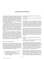
Table 1 summarizes the physical interpretation for a
variety of characteristic diameters. The Feret and Martin
diameters are typical geometric diameters obtained from
particle silhouettes under a microscope.

15
© 2006 by Taylor & Francis Group, LLC
16 AEROSOLS
When particles, at total number concentration N, are
measured based on a certain characteristic diameter as shown
in Table 1 and the number of particles, d n, having diameters
between D
p
and D
p
ϩ d D
p
are counted, the normalized par-
ticle size distribution f ( D
p
) is defined as follows:
fD
N
n
D
p
p
()
ϭ
1d
d
,
(1)
where
fDD

pp
()
∫
dϭ1
0
d
.
The discrete analog which gives a size distribution histo-
gram is
fD
N
n
D
p
p
()
ϭ
1⌬
⌬
(2)
where ⌬ n is the particle number concentration between D
p
Ϫ
⌬ D
p
/2 and D
p
ϩ⌬ D
p
/2.

The cumulative number concentration of particles up to
any diameter D
p
is given as
FDfDDfDD
pp
D
pp
D
p
p
p
()()()
∫∫
ϭϭϪ
a

aa
d
a
dd1
d
d
F
D
fD
p
p
ϭ
()

. (3)
The size distribution and the cumulative distribution
as defined above are based on the number concentration of
particles. If total mass M and fractional mass d m are used
instead of N and d n, respectively, the size distributions can
then be defined on a mass basis.
Many particle size distributions are well described by
the normal or the log-normal distributions. The normal, or
Gaussian, distribution function is defined as,
fD
DD
p
p
p
()
()
⎛
⎝
⎜
⎜
⎞
⎠
⎟
⎟
ϭϪ
Ϫ
1
2
2
2

2
ps
s
exp (4)
0.10.5151050
99.9
99
90
70
50
30
10
1
0.1
D
p
( m)
F=84.13%
D
g
D
g
MMD
NMD
D
mode
D
h
D
1

D
v
D
2
D
3
D
4
mass basis
number basis
100-F (%)
σ
g
x 2.0
D
8
µ
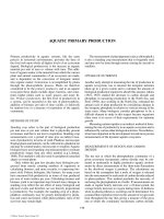
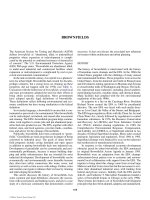
FIGURE 1 Log-normal size distribution for particles with geo-
metric mean diameter of 1 µ m and geometric standard deviation
of 2.0. The different average particle diameters for this distribution
are defined in Table 2.
TABLE 1 (continued)
Measures of particle size
Definition of characteristic diameters
Physical meaning and corresponding
measuring method
thickness: t
volume: v
aerodynamic diam. diameter of the sphere having unit specific
gravity and having the same gravitational

setting velocity as that of a particle, D
ae
ϭ
[18 mu
t
/gC
c
]
1/2
, obtained by the same
methods as the above.
surface
area: s
electrical mobility equivalent
diam.
diameter of the sphere having the same
electrical mobility as that of a particle, D
e
= n
p
eC
c
/3pmB
e
, obtained by electrical
mobility analyzer.
equivalent diffusion diam. diameter of the sphere having the same
penetration as that of a particle obtained
by diffusion battery.
equivalent light scattering

diam.
diameter of the sphere having the same
intensity of light scattering as that of a
standard particle such as a PSL particle,
obtained by light scattering method.
© 2006 by Taylor & Francis Group, LLC
where D
Ϫ
p
and s are, respectively, the mean and standard devi-
ation of the distribution. The mean diameter D
Ϫ
p
is defined by
DDfDD
p
ppp
ϭ
Ϫ
()
∫
d
d
d
(5)
and the standard deviation, indicating the dispersion of the
distribution, is given by
s
2
2

ϭϪ
Ϫ
DDfDD
p
p
pp
()
()
∫
d
d
d.
(6)
In the practical measurement of particle sizes, D
Ϫ
p
and s are
determined by
D
nD
N
nD D
N
p
ipi
ipi
p
ϭ
ϭ
ր

∑
()
⎛
⎝
⎜
⎜
⎞
⎠
⎟
⎟
s
Ϫ
2
12
(7)
where n
i
is the number of particles with diameter D
pi
and N
is the total particle number measured.
TABLE 2
Names and defining equations for various average diameters
Defining equations
General case In the case of log-normal distribution
number mean diam. D
1
⌺⌬nD
N
p

ln D
1
ϭ A ϩ 0.5C ϭ B Ϫ 2.5C
length mean diam. D
2
⌺⌬
⌺⌬
nD
nD
p
p
2
ln D
2
ϭ A ϩ 1.5C ϭ B Ϫ 1.5C
surface mean, Sauter or mean
volume-surface diam. D
3
⌺⌬
⌺⌬
ϭ
⌺⌬nD
nD
sD
S
p
p
p
3
2

ln D
3
ϭ A ϩ 2.5C ϭ B Ϫ 0.5C
volume or mass mean diam. D
4
⌺⌬
⌺⌬
ϭ
⌺⌬nD
nD
mD
M
p
p
p
4
3
ln D
4
ϭ A ϩ 3.5C ϭ B ϩ 0.5C
diam. of average surface D
s
⌺⌬nD
N
p
2
ln D
s
ϭ A ϩ 1.0C ϭ B Ϫ 2.0C
diam. of average volume or mass D

v
⌺⌬nD
N
p
3
3
ln D
v
ϭ A ϩ 1.5C ϭ B Ϫ 1.5C
harmonic mean diam. D
h
N
D
p
⌺⌬(/ )
ln D
h
ϭ A Ϫ 0.5C ϭ B Ϫ 3.5C
number median diam. or geometric
mean diam. NMD
exp
ln⌺⌬nD
N
p
⎡
⎣
⎢
⎤
⎦
⎥

NMD
volume or mass median diam. MMD
exp
ln⌺⌬
⌺⌬
nD D
nD
pp
p
3
3
⎡
⎣
⎢
⎤
⎦
⎥
ln MMD ϭ A ϩ 3C
ϭ
⌺⌬
exp
lnmD
M
p
⎡
⎣
⎢
A ϭ ln NMD, B ϭ ln MMD, C ϭ (ln s
g
)

2
N(total number) ϭ⌺⌬n, S(total surface) ϭ⌺⌬s, M(total mass) ϭ⌺⌬m
AEROSOLS 17
© 2006 by Taylor & Francis Group, LLC
The log-normal distribution is particularly useful for rep-
resenting aerosols because it does not allow negative particle
sizes. The log-normal distribution function is obtained by
substituting ln D
p
and ln ␴
g
for D
p
and s in Eq. (4),
.
fD
DD
p
g
p
p
g
ln
ln
ln
.
()
()
⎛
⎝

⎜
⎜
⎞
⎠
⎟
⎟
ϭϪ
Ϫ
1
2
2
2
2
πs
s
exp
lnln
(8)
The log-normal distribution has the following cumulative
distribution,
F
DD
D
g
pg
g
D
p
p
ϭϪ

Ϫ
1
2
2
2
2
0
ps
s
ln
exp
lnln
ln
.
()
⎛
⎝
⎜
⎜
⎞
⎠
⎟
⎟
()
∫
dln
(9)
The geometric mean diameter D
g
, and the geometric standard

deviation s
g
, are determined from particle count data by
lnln
lnlnln.
DnDN
nDDN
gipi
gipig
ϭ
ϭϪ
ր
∑
∑
()
()
⎡
⎣
⎢
⎤
⎦
⎥

s
2
12
(10)
Figure 1 shows the log-normal size distribution for par-
ticles having D
g

ϭ 1 mm and s
g
ϭ 2.0 on a log-probability
graph, on which a log-normal size distribution is a straight
line. The particle size at the 50 percent point of the cumu-
lative axis is the geometric mean diameter D
g
or number
median diameter, NMD. The geometric standard deviation
is obtained from two points as follows:
s
g
p
p
p
po
DF
DF
DF
DF
ϭ
ϭ
ϭ
ϭ
ϭ
ϭ
at
at
at
at

8413
50
50
157
.%
%
%
.%
.
The rapid graphical determination of the geometric
mean diameter D
g
as well as the standard deviation s
g
is a
major advantage of the log-normal distribution. It should
be emphasized that the size distribution on a number basis
shown by the solid line in Figure 1 differs significantly
from that on a mass basis, shown by the dashed line in the
same figure. The conversion from number median diameter
(NMD) to mass median diameter (MMD) for a log-normal
distribution is given by
ln(MMD) ϭ ln(NMD) ϩ 3(ln s
g
)
2
. (11)
If many particles having similar shape are measured on the
basis of one of the characteristic diameters defined in Table 1,
a variety of average particle diameters can be calculated as

shown in Table 2. The comparison among these diameters is
shown in Figure 1 for a log-normal size distribution. Each
average diameter can be easily calculated from s
g
and NMD
(or MMD).
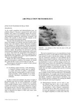
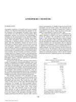
Figure 2 indicates approximately the major sources of
atmospheric aerosols and their surface area distributions.
There tends to be a minimum in the size distribution of
atmospheric particles around 1 mm, separating on one hand
the coarse particles generated by storms, oceans and volca-
noes and on the other hand the fine particles generated by
fires, combustion and atmospheric chemistry. The commi-
nution processes generate particles in the range above 1 mm
and molecular processes lead to submicron particles.
PARTICLE DYNAMICS AND PROPERTIES
Typical size-dependent dynamic properties of particles sus-
pended in a gas are shown in Figure 3 together with defining
equations (Seinfeld, 1986). The solid lines are those at atmo-
spheric pressure and the one-point dashed lines are at low
pressure. The curves appearing in the figure and the related
particle properties are briefly explained below.
Motion of Large Particles
A single spherical particle of diameter D
p
with a velocity uin
air of density r
f
experiences the following drag force,
F

d
ϭ C
D
A
p
(r
f
u
2
/2) (12)
10
–3
10
–2
10
–1
10
–1
10
0
10
0
10
1
10
2
10
3
10
4

10
5
10
1
10
2
10
3
D
p
(mm)
FOREST FIRE
PLUMES
INTENSE
SMOG
HEAVY
AUTO
TRAFFIC
VOLCANIC PLUMES
DUST STORMS
SAND
STORMS
INDUSTRY
TYPICAL URBAN
POLLUTION
SEA SALT
SOUTH ATLANTIC
BACKGROUND
NORTH ATLANTIC
BACKGROUND

CONTINENTAL
BACKGROUND
SURFACE AREA DISTRIBUTION, ∆S/∆log D
p
(mm
2
cm
–3
)
FIGURE 2 Surface area distributions of natural and anthropo-
genic aerosols.
18 AEROSOLS
© 2006 by Taylor & Francis Group, LLC
0.001
10
–8
10
–7
10
–6
10
–5
10
–4
10
–3
10
–2
10
–1

10
0
0.01 0.1
1
10
D
p
(mm)
Kelvin
effect,
(water
droplet)
Relaxation time
C
c
at 10mm Hg
Diffusion coeff., D
(n
p
=1
)
Pulse height
(example)
Slip coeff., C
c
τ
g
at 10mm H
g
τ

g
1°C/cm
V
th
Average absolute value of Brownian
displacement in 1s, ∆X in air
20°C in air
1atm
10 mm Hg
Settling velocity, V
t
In air (
p
=1g cm
–3
)
1
10
10
–2
10
–1
10
0
10
1
10
2
100
1000

1
2
3
4
5
6
7
8
Slip coefficient, C
c
Pulse height (light scattering)
Increase in vapor pressure by Kelvin effect, p
d
/p
Settling velocity v
t
(cm/s), Diffusion coefficient D (cm
2
/s),
Relaxation time τ
g
(s), Electrical mobility B
e
(cm
2
V
–1
s
–1
),

Average absolute value of Brownian displacement in 1s ∆x=
4D/p
(cm),
Thermophoretic velocity v
th
(cm/s)
V
t
=
(
p
–
f
)gD
p
C
c
18m
18m
(3.1)
(3.4)
(3.6)
(3.8)
C
c
=1+2.514
λ
D
p
D

p
λ
λ
D
p
+0.80 exp(–0.55
)
(3.2)
(3.3)
(3.5)
(3.7)
C
c
=1+(2 / pD
p
) [6.32 + 2.01 exp (–0.1095pD
p
)] p in cm Hg, D
p
in mm
∆x =
4Dt
D =
kTC
c
τ
g
=
p
D

p
C
c
B
e
=
n
p
e C
c
P
d
/P
8
= exp (
4Mσ
RT
l
D
p
)
p
=1g cm
–3
Electrical mobility, B
e
3pmDp
3pmDp
ρ
ρ

ρ
ρ
2
2
ρ
ρ
8
p
FIGURE 3 Fundamental mechanical and dynamic properties of aerosol particles suspended in a gas.
AEROSOLS 19
© 2006 by Taylor & Francis Group, LLC
TABLE 3
Motion of a single spherical particle
Re
p
Ͻ 1 (Stokes) 1 Ͻ Re
p
Ͻ 10
4
10
4
Ͻ Re
p
(Newton)
drag coefficient, C
D
24/Re
p
055
48

2
.
.
ϩ
Re
p
⎛
⎝
⎜
⎜
⎞
⎠
⎟
⎟
0.44
drag force,
RCA
f
Dp
f
v
ϭ
r
2
2
3pmD
p
v
055 48
8

2

vD D v
pf p
r
m
pm
ϩ
⎛
⎝
⎜
⎞
⎠
⎟
0.055pr
f
(vD
p
)
2
gravitational settling equation of
motion
m
v
t
mgR
pp
f
p
f

d
d
ϭϪϪ1
r
r
⎛
⎝
⎜
⎞
⎠
⎟
or,
d
d
v
t
ϭϪ Ϫ1
3
4
2
r
r
r
r
f
p
f
pp
D
g

D
Cv
⎛
⎝
⎜
⎞
⎠
⎟
terminal velocity, v
t
(dv/dt ϭ 0)
Dg
pp f
2
18
rr
m
Ϫ
()
AAA
1
2
21
2
11
+
⎛
⎝
⎜
⎜

⎞
⎠
⎟
⎟
Ϫ
.
A
D
fp
1
48ϭ .
m
r
AgD
pf
f
p2
254ϭ
Ϫ
.
rr
r
3
12
Dg
pp f
f
()
/
rr

r
Ϫ
⎛
⎝
⎜
⎞
⎠
⎟
unsteady motion
time, t
velocity, v
t
vv
vv
g
t
t
ϭ
Ϫ
Ϫ
t 1
0
n
⎛
⎝
⎜
⎞
⎠
⎟
t

CC
g
p
Dt t D p
p
p
ϭ
Ϫ
24
22
0
t
dRe
Re Re
Re
Re
∫
not simple because of Re
p
ϽϽ 10
4
at initiation of motion
falling distance, S
St
t
ϭ vd
0
∫
vt v v
t

tgt
g
ϭϪ ϪϪt
t
()exp
0
1
⎛
⎝
⎜
⎞
⎠
⎟
⎡
⎣
⎢
⎢
⎤
⎦
⎥
⎥
vt
tt
tg p
t
gp pp
t
t
Re
/ ,Re Re / Re

d
0
0
∫
ϭϭ
Re
18
initial velocity, : terminal v
2
p
pf
g
pp
t
vD D
vvϭϭ
r
m
t
r
m
,,:
0
eelocity
Re
p0
, Re
pt
: Re
p

at v
0
and at v
t
respectively, C
Dt
: drag coefficient at terminal velocity
20 AEROSOLS
where A
p
is the projected area of the particle on the flow (ϭ
pD
p
2
/4), and C
D
is the drag coefficient of the particle. The
drag coefficient C
D
depends on the Reynolds number,
Re /ϭ uD
rpf
rm (13)
where u
r
is the relative velocity between the particle and air
( ϭ | u Ϫ v |, u ϭ velocity of air flow, v ϭ particle velocity),
and m is the viscosity of the fluid.
The motion of a particle having mass m
p

is expressed by
the equation of motion
m
t
p
d
d
v
Fϭ
∑
(14)
where v is the velocity of the particle and F is the force acting
on the particle, such as gravity, drag force, or electrical force.
Table 3 shows the available drag coefficients depending on
© 2006 by Taylor & Francis Group, LLC
AEROSOLS 21
from t ϭ 1s in Eq. (3.4). The intersection of the curves ⌬
Ϫ
x
Ϫ
and v
t
lies at around 0.5 mm at atmospheric pressure. If one
observes the settling velocity of such a small particle in a
short time, it will be a resultant velocity caused by both grav-
itational settling and Brownian motion.
The local deposition rate of particles by Brownian diffu-
sion onto a unit surface area, the deposition flux j (number of
deposited particles per unit time and surface area), is given by
j ϭ – D ٌ N ϩ vN ϩ uN. (19)

If the flow is turbulent, the value of the deposition flux of
uncharged particles depends on the strength of the flow
field, the Brownian diffusion coefficient, and gravitational
sedimentation.
Particle Charging and Electrical Properties
When a charged particle having n
p
elementary charges is sus-
pended in an electrical field of strength E, the electrical force
F
e
exerted on the particle is n
p
eE, where e is the elemen-
tary charge unit ( e ϭ 1.6 ϫ 10
Ϫ19
C). Introducing F
e
into the
right hand side of the equation of particle motion in Table 3
and assuming that gravity and buoyant forces are negligible,
the steady state velocity due to electrical force is found by
equating drag and electrical forces, F
d
ϭ F
e
. For the Stokes
drag force ( F
d
ϭ 3pmv

e
D
p
/ C
c
), the terminal electrophoretic
velocity v
e
is given by
v
e
ϭn
p
eEC
c
/3pmD
p
. (20)
B
e
in Figure 3 is the electrical mobility which is defined
as the velocity of a charged particle in an electric field of
unit strength. Accordingly, the steady particle velocity in an
electric field E is given by Eb
e
. Since B
e
depends upon the
number of elementary charges that a particle carries, n
p

, as
seen in Eq. (3.7), n
p
is required to determine B
e
. n
p
is predict-
able with aerosol particles in most cases, where particles are
charged by diffusion of ions.
The charging of particles by gaseous ions depends on
the two physical mechanisms of diffusion and field charging
(Flagan and Seinfeld, 1988). Diffusion charging arises from
thermal collisions between particles and ions. Charging occurs
also when ions drift along electric field lines and impinge upon
the particle. This charging process is referred to as field charg-
ing. Diffusion charging is the predominant mechanism for
particles smaller than about 0.2 mm in diameter. In the size
range of 0.2–2 mm diameter, particles are charged by both dif-
fusion and field charging. Charging is also classified into bipo-
lar charging by bipolar ions and unipolar charging by unipolar
ions of either sign. The average number of charges on particles
by both field and diffusion charging are shown in Figure 4.
When the number concentration of bipolar ions issufficiently
high with sufficient charging time, the particle charge attains
an equilibrium state where the positive and negative charges
in a unit volume are approximately equal. Figure 5 shows the
charge distribution of particles at the equilibrium state.
Reynolds number and the basic equation expressing the par-
ticle motion in a gravity field.

The terminal settling velocity under gravity for small
Reynolds number, v
t
, decreases with a decrease in particle
size, as expressed by Eq. (3.1) in Figure 3. The distortion
at the small size range of the solid line of v
t
is a result of
the slip coefficient, C
c
, which is size-dependent as shown in
Eq. (3.2). The slip coefficient C
c
increases with a decrease
in particle size suspended in a gaseous medium. It also
increases with a decrease in gas pressure p as shown in
Figure 3. The terminal settling velocities at other Reynolds
numbers are shown in Table 3.
t
g
in Figure 3 is the relaxation time and is given by
Eq. (3.6). It characterizes the time required for a particle to
change its velocity when the external forces change. When
a particle is projected into a stationary fluid with a velocity
v
o
, it will travel a finite distance before it stops. Such a dis-
tance called the stop-distance and is given by v
0
t

g
. Thus, t
g
is a measure of the inertial motion of a particle in a fluid.
Motion of a Small Diffusive Particle
When a particle is small, Brownian motion occurs caused
by random variations in the incessant bombardment of mol-
ecules against the particle. As the result of Brownian motion,
aerosol particles appear to diffuse in a manner analogous to
the diffusion of gas molecules.
The Brownian diffusion coefficient of particles with
diameter D
p
is given by
Dϭ C
c
kT/3pmD
p
(15)
where k is the Boltzmann constant (ϭ1.38ϫ 10
Ϫ16
erg/K) and
T the temperature [K]. The mean square displacement of a
particles⌬
Ϫ
x
ᎏ
2
in a certain time interval t, and its absolute value
of the average displacement ⌬

Ϫ
x
Ϫ
, by the Brownian motion, are
given as follows
⌬
⌬
xDt
xDt
2
2
4
ϭ
ϭcp
(16)
The number concentration of small particles undergoing
Brownian diffusion in a flow with velocity u can be determined
by solving the following equation of convective diffusion,
Ѩ
Ѩ
ϩٌϭٌϪٌ
N
t
NDNN⋅⋅uv
2
(17)
vFϭτ
gp
mc
∑

(18)
where N is the particle number concentration, D the Brownian
diffusion coefficient, and v the particle velocity due to an
external force F acting on the particle.
The average absolute value of Brownian displacement
in one second, ⌬
Ϫ
x
Ϫ
, is shown in Figure 3, which is obtained
© 2006 by Taylor & Francis Group, LLC
22 AEROSOLS
Brownian Coagulation
Coagulation of aerosols causes a continuous change in
number concentration and size distribution of an aerosol with
the total particle volume remaining constant. Coagulation
can be classified according to the type of force that causes
collision. Brownian coagulation (thermal coagulation) is a
fundamental mechanism that is present whenever particles
are present in a background gas.
In the special case of the initial stage of coagulation of a
monodisperse aerosol having uniform diameter D
p
, the par-
ticle number concentration N decreases according to
ddNt KN
KKDD
pp
c ϭϪ
ϭ

05
0
2
0
.
,
()
(21)
where K ( D
p
, D
p
) is the coagulation coefficient between par-
ticles of diameters D
p
and D
p
.
When the coagulation coefficient is not a function of
time, the decrease in particle number concentration from N
0
to N can be obtained from the integration of Eq. (21) over a
time period from 0 to t ,
N ϭ N
0
/(1 ϩ 0.5 K
0
N
0
t ). (22)

The particle number concentration reduces to one-half its ini-
tial value at the time 2( K
0
N
0
)
Ϫ1
. This time can be considered
as a characteristic time for coagulation.
In the case of coagulation of a polydisperse aerosol, the
basic equation that describes the time-dependent change in
the particle size distribution n ( v, t ), is
Ѩ
Ѩ
ϭϪ Ϫ
Ϫ
nvt
t
Kvvvnvtnvvtdv
nvt Kvv
v
,
,
,,
(
)
(
)
(
)

(
)
(
)
(
)
∫
1
2
0
a a a a a
a
00
d
a a
∫
(
)
nv tdv
(23)
The first term on the right-hand side represents the rate of
formation of particles of volume v due to coagulation, and
the second term that rate of loss of particles of volume v by
coagulation with all other particles.
The Brownian coagulation coefficient is a function of
the Knudsen number Kn ϭ 2l/ D
p
, where l is the mean free
path of the background gas. Figure 6 shows the values of
the Brownian coagulation coefficient of mono-disperse par-

ticles, 0.5 K ( D
p
, D
p
), as a function of particle diameter in
10
–2
10
–1
10
0
10
1
10
–2
10
–1
10
0
10
1
10
2
10
3
D
p
(mm)
Equilibrium charge
distribution by

bipolar ions
Diffusion charging by
unipolar ions
N
S
t=10
13
s/m
3
N
S
: ion number concentration
1 : charging time
Field charging by
unipolar ions
E = 3ϫ10
5
V/m
N
S
t = 10
13
s/m
n
␳
n
␳
n(n
␳
) n(n

␳
)
n
␳
⌺
ϱ
ϱϱ
=
=–
n
␳
⌺
ϱ
=–
/
FIGURE 4 The average number of charges on particles by both
field and diffusion charging .
FIGURE 5 Equilibrium charge distribution through bipolar ion
charging. The height of each section corresponds to the number
concentration of particles containing the indicated charge. .
0.02 0.04 0.1
0.2 0.5
12
D
p
(mm)
Particle number concentration
м2
n
p

м3
n
p
м4
м4
n
p
n
p
n
p
+2
+1
+3
–3
–2
–1
–1
+1
+1
–1
+2
–2
0
0
+3
–3
+1
–1
+2

–2
0
0
0
0
Ϯ1
Ϯ4
Ϯ3
Ϯ2
Ϯ1
Particle size distribution
Charge distribution
м5
FIGURE 6 Brownian coagulation coefficient for coagulation of
equal-sized particles in air at standard conditions as a function of
particle density.
0.001 0.01 0.1 1.0
D
p
(mm)
10
–10
10
–9
10.0
5.0
2.5
1.0
0.5
p

= 0.25
20 10 5 4 3 2 1 0.5 .4.3 .2 0.1
Knudsen number Kn
0.5K
B
(D
p
, D
p
) (cm
3
/s)
ρ
© 2006 by Taylor & Francis Group, LLC
AEROSOLS 23
air at atmospheric pressure and room temperature. There
exist distinct maxima in the coagulation coefficient in the
size range from 0.01 mm to 0.01 mm depending on particle
diameter. For a particle of 0.4 mm diameter at a number con-
centration of 10
8
particles/cm
3
, the half-life for Brownian
coagulation is about 14 s.
Kelvin Effect
p
d
/ p
ϱ

in Figure 3 indicates the ratio of the vapor pressure over
a curved droplet surface to that over a flat surface of the same
liquid. The vapor pressure over a droplet surface increases with
a decrease in droplet diameter. This phenomenon is called the
Kelvin effect and is given by Eq. (3.8). If the saturation ratio
of water vapor S surrounding a single isolated water droplet
is larger than p
d
/ p
ϱ
, the droplet grows. If S < p
d
/ p
ϱ
, that is,
the surrounding saturation ratio lies below the curve p
d
/ p
ϱ
in
Figure 3, the water droplet evaporates. Thus the curve p
d
/ p
ϱ
in
Figure 3 indicates the stability relationship between the drop-
let diameter and the surrounding vapor pressure.
Phoretic Phenomena
Phoretic phenomena refer to particle motion that occurs
when there is a difference in the number of molecular colli-

sions onto the particle surface between different sides of the
particle. Thermophoresis, photophoresis and diffusiophore-
sis are representative phoretic phenomena.
When a temperature gradient is established in a gas, the
aerosol particles in that gas are driven from high to low tem-
perature regions. This effect is called thermophoresis. The
curve v
th
in Figure 3 is an example (NaCl particles in air) of
the thermophoretic velocity at a unit temperature gradient,
that is, 1 K/cm. If the temperature gradient is 10 K/cm, v
th
becomes ten times higher than shown in the figure.
If a particle suspended in a gas is illuminated and non-
uniformly heated due to light absorption, the rebound of gas
molecules from the higher temperature regions of the par-
ticle give rise to a motion of the particle, which is called
photophoresis and is recognized as a special case of thermo-
phoresis. The particle motion due to photophoresis depends
on the particle size, shape, optical properties, intensity and
wavelength of the light, and accurate prediction of the phe-
nomenon is rather difficult.
Diffusiophoresis occurs in the presence of a gradient of
vapor molecules. The particle moves in the direction from
higher to lower vapor molecule concentration.
OPTICAL PHENOMENA
When a beam of light is directed at suspended particles, vari-
ous optical phenomena such as absorption and scattering of
the incident beam arise due to the difference in the refrac-
tive index between the particle and the medium. Optical

phenomena can be mainly characterized by a dimensionless
parameter defined as the ratio of the particle diameter D
p
to
the wavelength of the incident light l,
a ϭ pD
p
/l. (24)
Light Scattering
Light scattering is affected by the size, shape and refractive
index of the particles and by the wavelength, intensity, polar-
ization and scattering angle of the incident light. The theory
of light scattering for a uniform spherical particle is well
established (Van de Hulst, 1957). The intensity of the scat-
tered light in the direct u (angle between the directions of the
incident and scattered beams) consists of vertically polarized
and horizontally polarized components and is given as
II
r
iiϭϩ
0
2
22
12
8
l
p
()
(25)
where I

0
denotes the intensity of the incident beam, l the
wavelength and r the distance from the center of the particle,
i
1
and i
2
indicate the intensities of the vertical and horizontal
components, respectively, which are the functions of u, l,
D
p
and m.
The index of refraction m of a particle is given by the
inverse of the ratio of the propagation speed of light in a
vacuum k
0
to that in the actual medium k
1
as,
m ϭ k
1
/ k
0
(26)
and can be written in a simple form as follows:
m ϭ n
1
Ϫ in
2
. (27)

The imaginary part n
2
gives rise to absorption of light, and
vanishes if the particle is nonconductive.
Light scattering phenomena are sometimes separated into
the following three cases: (1) Rayleigh scattering (molecu-
lar scattering), where the value of a is smaller than about 2,
(2) Mie scattering, where a is from 2 to 10, and (3) geo-
metrical optics (diffraction), where a is larger than about 10.
In the Rayleigh scattering range, the scattered intensity is
in proportion to the sixth power of particle size. In the Mie
scattering range, the scattered intensity increases with parti-
cle size at a rate that approaches the square of particle size as
the particle reaches the geometrical optics range. The ampli-
tude of the oscillation in scattered intensity is large in the
forward direction. The scattered intensity greatly depends on
the refractive index of the particles.
The curve denoted as pulse height in Figure 3 illustrates
a typical photomultiplier response of scattered light from a
particle. The intensity of scattered light is proportional to
the sixth power of the particle diameter when particle size is
smaller than the wavelength of the incident light (Rayleigh
scattering range). The curve demonstrates the steep decrease
in intensity of scattered light from a particle.
Light Extinction
When a parallel beam of light is passed through a suspen-
sion, the intensity of light is decreased because of the scat-
tering and absorption of light by particles. If a parallel light
© 2006 by Taylor & Francis Group, LLC
24 AEROSOLS

beam of intensity I
0
is applied to the suspension, the intensity
I at a distance l into the medium is given by,
I ϭ I
0
exp(Ϫgl) (28)
where g is called the extinction coefficient,
gϭCnDD
ppext
d
()
∫
0
d
(29)
n ( D
p
) is the number distribution function of particles, and
C
ext
is the cross sectional area of each particle.
For a spherical particle, C
ext
can be calculated by the Mie
theory where the scattering angle is zero. The value of C
ext
is also given by
C
ext

ϭ C
sca
ϩ C
abs
(30)
where C
sca
is the cross sectional area for light scattering and
C
abs
the cross sectional area for light absorption. The value of
C
sca
can be calculated by integrating the scattered intensity I
over the whole range of solid angles.
The total extinction coefficient g in the atmosphere can
be expressed as the sum of contributions for aerosol particle
scattering and absorption and gaseous molecular scattering and
absorption. Since the light extinction of visible rays by polluted
gases is negligible under the usual atmospheric conditions and
the refractive index of atmospheric conditions and the refrac-
tive index of atmospheric aerosol near the ground surface is
(1.33∼ 1.55) Ϫ (0.001 ∼ 0.05) i (Lodge et al., 1981), the extinc-
tion of the visible rays depends on aerosol particle scattering
rather than absorption. Accordingly, under uniform particle
concentrations, the extinction coefficient becomes a maximum
for particles having diameter 0.5 mm for visible light.
VISIBILITY
The visible distance that can be distinguished in the atmo-
sphere is considerably shortened by the light scattering and

light extinction due to the interaction of visible light with
the various suspended particles and gas molecules. To evalu-
ate the visibility quantitatively, the visual range, which is
defined as the maximum distance at which the object is just
distinguishable from the background, is usually introduced.
This visual range is related to the intensity of the contrast C
for an isolated object surrounded by a uniform and extensive
background. The brightness can be obtained by integrating
Eq. (28) over the distance from the object to the point of
observation. If the minimum contrast required to just dis-
tinguish an object from its background is denoted by C
*
, the
visual range L
v
for a black object can be given as
L
v
ϭϪ(1/g)ln(Ϫ C
*
) (31)
where g is the extinction coefficient. Introduction of the
value of Ϫ0.02 for C
*
gives the well known Koschmieder
equation,
L
v
ϭ 3.912/g (32)
For aerosol consisting of 0.5 mm diameter particles ( m ϭ

1.5) at a number concentration of 10
4
particles/cm
3
, the
extinction coefficient g is 6.5 ϫ 10
Ϫ5
cm and the daylight
visual range is about 6.0 ϫ 10
4
cm (ϭ0.6 km). Since the
extinction coefficient depends on the wavelength of light,
refractive index, aerosol size and concentration, the visual
range greatly depends on the aerosol properties and atmo-
spheric conditions.
MEASUREMENT OF AEROSOLS
Methods of sizing aerosol particles are generally based upon
the dynamic and physical properties of particles suspended
in a gas (see Table 4).
Optical Methods
The light-scattering properties of an individual particle are a
function of its size, shape and refractive index. The intensity of
scattered light is a function of the scattering angle, the inten-
sity and wavelength of the incident light, in addition to the
above properties of an individual particle. An example of the
particle size-intensity response is illustrated in Figure 3. Many
different optical particle sizing devices have been developed
based on the Mie theory which describes the relation among
the above factors. The principle of one of the typical devices
is shown in Figure 7.

The particle size measured by this method is, in most
cases, an optical equivalent diameter which is referred to a
calibration particle such as one of polystyrene latex of known
size. Unless the particles being measured are spheres of
known refractive index, their real diameters cannot be evalu-
ated from the optical equivalent diameters measured. Several
light-scattering particle counters are commercially available.
Inertial Methods (Impactor)
The operating principle of an impactor is illustrated in
Figure 8. The particle trajectory which may or may not col-
lide with the impaction surface can be calculated from solv-
ing the equation of motion of a particle in the impactor flow
field. Marple’s results obtained for round jets are illustrated
in Figure 8 (Marple and Liu, 1974), where the collection
efficiency at the impaction surface is expressed in terms of
the Stokes number, Stk, defined as,
Stk
CDu
W
u
W
pc p
ϭϭ
r
m
t
2
0
0
18 2 2cc

(
)
(33)
where
t
r
m
ϭ
ppc
DC
2
18
(34)
C
DD
D
c
pp
p
ϭϩ ϩ Ϫ1 2 514.
ll
l
0.80 exp 0.55
⎛
⎝
⎜
⎞
⎠
⎟
(35)

© 2006 by Taylor & Francis Group, LLC
AEROSOLS 25
r
p
is the particle density, m the viscosity and l is the mean
free path of the gas. The remaining quantities are defined in
Figure 8.
The value of the Stokes number at the 50 percent collection
efficiency for a given impactor geometry and operating condi-
tion can be found from the figure, and it follows that the cut-off
size, the size at 50 percent collection efficiency, is determined.
If impactors having different cut-off sizes are appropri-
ately connected in series, the resulting device is called a cas-
cade impactor, and the size distribution of aerosol particles
can be obtained by weighing the collected particles on each
impactor stage. In order to obtain an accurate particle size dis-
tribution from a cascade impactor, the following must be taken
into account: 1) data reduction considering cross sensitivity
between the neighboring stages, 2) rebounding on the impac-
tion surfaces, and 3) particle deposition inside the device.
Various types of impactors include those using multiple
jets or rectangular jets for high flow rate, those operating under
low pressure (Hering et al., 1979) or having microjets for par-
ticles smaller than about 0.3 mm and those having a virtual
impaction surface, from which aerosols are sampled, for sam-
pling the classified aerosol particles (Masuda et al., 1979).
TABLE 4
Methods of aerosol particle size analysis
Quantity to be
measured

Method or
instrumentMediaDetection
Approx size
rangeConcentrationPrinciple
microscopegasnumberϾ0.5mm
lengthelectron microscopevacuumnumberϾ0.001
absorbed gasadsorption method,
BET
gas–Ͼ0.01BET
arealiquid
permeabilitypermeability methodgas–Ͼ0.1Kozeny-
Carman’s
equation
volumeelectric resist.Coulter CounterliquidnumberϾ0.3low
gravitational(individual)
ultramicroscope
gasnumberϾ1lowStokes equation
settling(differential conc.)liquidmassϾ1highStokes equation
motion in fluidvelocity(cumulative conc.)liquidmassϾ1highStokes equation
centrifugal(differential conc.)liquidarea massϾ0.05highStokes equation
settling velocityspiral centrifuge,
conifuge
gasnumber massϾ0.05–1high–lowStokes equation
inertial collectionimpactor, acceleration
method
gasmass numberϾ0.5high–lowrelaxation time
inertial motionimpactor, aerosol
beam method
gasnumberϾ0.05high–lowin low pressure
diffusion lossdiffusion battery and

CNC
gasmass number0.002–0.5high–lowBrownian
motion
Brownian motionphoton correlationliquidnumber0.02–1high
integral type (EAA)gasnumber (current)0.005–0.1high–low
electric mobility
differential type
(DMA)
gasnumber (current)0.002–0.5high–low
intensity of scattered
light
light scatteringgas liquidnumber>0.1lowMie theory
light diffractiongas liquidnumber1high–low
(Other Inertial Methods)
Other inertial methods exist for particles larger than 0.5
mm, which include the particle acceleration method,
multi-cyclone (Smith et al., 1979), and pulsation method
(Mazumder et al. , 1979). Figure 9illustrates the particle
acceleration method where the velocity difference between
PULSE VOLTAGE
PARTICLE DIAMETER
TIME
PULSE VOLTAGE
FREQUENCY
PARTICLE
NUMBER
SENSING
VOLUME
LIGHT TRAP
INCIDENT BEAM

AEROSOL
θ
PHOTOMULTIPLIER
FIGURE 7 Measurement of aerosol particle size by an optical
method.
© 2006 by Taylor & Francis Group, LLC
26 AEROSOLS
a particle and air at the outlet of a converging nozzle is
detected (Wilson and Liu, 1980).
Sedimentation Method
By observing the terminal settling velocities of particles it
is possible to infer their size. This method is useful if a TV
camera and He–Ne gas laser for illumination are used for the
observation of particle movement. A method of this type has
been developed where a very shallow cell and a TV system
are used (Yoshida et al., 1975).
Centrifuging Method
Particle size can be determined by collecting particles in a
centrifugal flow field. Several different types of centrifugal
IMPACTION SURFACE
SMALL
PARTICLE
S
T
LARGE
PARTICLE
STREAMLINE
OF GAS
MEAN GAS FLOW
U

0
W
Re =
25000
3000
500
10
S/W=0.5, T/W=1
Re=3000, T/W=2
0.30.40.50.60.70.80.9
Stk
0
20
40
60
80
100
S/W=
0.25
0.5
5.0
COLLECTION EFFICIENCY (%)
FIGURE 8 Principle of operation of an impactor. Collection effi-
ciency of one stage of an impactor as a function of Stokes number,
Stk, Reynolds number, Re, and geometric ratios.
BEAM
SPLITTER
He–Ne
LASER
CLEAN

AIR
AEROSOL
NOZZLE
PHOTOMULTIPLIER
SIGNAL PROCESSING
CHAMBER PRESSURE
GAUGE
PUMP
FIGURE 9 Measurement of aerosol particle size by laser-
doppler velocimetry.
chambers, of conical, spiral and cylindrical shapes, have been
developed for aerosol size measurement. One such system is
illustrated in Figure 10 (Stöber, 1976). Particle shape and
chemical composition as a function of size can be analyzed
in such devices.
Electrical Mobility Analyzers
The velocity of a charged spherical particle in an electric field,
v
e
, is given by Eq. (20). The velocity of a particle having unit
charge ( n
p
ϭ 1) in an electric field of 1 V/cm is illustrated
in Figure 3. The principle of electrical mobility analyzers is
based upon the relation expressed by Eq. (20). Particles of
different sizes are separated due to their different electrical
mobilities.
FIGURE 10 Spiral centrifuge for particle size measurements.
AEROSOL
DISTRIBUTOR

CLEAN AIR
AEROSOL
CLEAN AIR
ROTATION
PLASTIC FILM
EXHAUST
DISTRIBUTOR
© 2006 by Taylor & Francis Group, LLC
AEROSOLS 27
SCREEN
UNIPOLAR
IONS
DC H.V.
AEROSOL
AEROSOL
RADIOACTIVE SOURCE
BIPOLAR IONS
DC H.V.
Q
c
Q
a
AEROSOL
CLEAN AIR
DC H.V.
Q
c
Q
a
AEROSOL

CLEAN AIR
r
1
r
2
L
EXHAUST, Q
c
TO DETECTOR
UNCHARGED PARTICLE
TO DETECTOR
Q
a
+ Q
c
AEROSOL
CNC
ELECTROMETER
FILTER
AEROSOL
a) Corona discharge (unipolar ions) b) Radioactive source (bipolar ions)
(a) Charging section for particles
a) Integration type
b) Differential type
(b) Main section
a) Electrometer
b) CNC or Electrometer
(c) Detection of charged particles
ELECTRICAL CURRENT
or PARTICLE NUMBER

ELECTRICAL CURRENT
or PARTICLE NUMBER
APPLIED VOLTAGE
APPLIED VOLTAGE
a) Integration type
b) Differential type
(d) Response curve
L
FIGURE 11 Two types of electrical mobility analyzers for determining aerosol size. Charging,
classification, detection and response are shown for both types of analyzers.
© 2006 by Taylor & Francis Group, LLC
28 AEROSOLS
Two different types of electrical mobility analyzers
shown in Figure 11 have been widely used (Whitby, 1976).
On the left hand side in the figure is an integral type, which is
commercially available (EAA: Electrical Aerosol Analyzer).
That on the right hand side is a differential type, which is
also commercially available (DMA: Differential Mobility
Analyzer). The critical electrical mobility B
ec
at which a par-
ticle can reach the lower end of the center rod at a given
operating condition is given, respectively, for the EAA and
DMA as
B
QQ
LV
r
r
ec

ac
ϭ
ϩ
()
⎛
⎝
⎜
⎞
⎠
⎟
2
1
2
p
ln
(36)
B
Q
LV
r
r
B
Q
LV
r
r
ec
c
e
a

ϭϭ
2
1
2
1
2
pp
ln,ln
⎛
⎝
⎜
⎞
⎠
⎟
⎛
⎝
⎜
⎞
⎠
⎟
⌬
(37)
B
ec
can be changed by changing the electric voltage applied
to the center rod. A set of data of the particle number con-
centration or current at every B
ec
can be converted into a size
distribution by data reduction where the number distribution

of elementary charges at a given particle size is taken into
account.
Electrical mobility analyzers are advantageous for
smaller particles because v
e
in Eq. (20) increases with the
decrease in particle size. The differential mobility analyzer
has been increasingly utilized as a sizing instrument and a
monodisperse aerosol generator of particles smaller than
1mm diameter (Kousaka et al. , 1985).
Diffusion Batteries
The diffusion coefficient of a particle D is given by Eq. (15).
As shown in Figure 3, D increases with a decrease in par-
ticle size. This suggests that the deposition loss of particles
onto the surface of a tube through which the aerosol is flow-
ing increases as the particle size decreases. The penetration
(ϭ1–fractional loss by deposition) h
p
for a laminar pipe flow
is given as (Fuchs, 1964),
h
p
ϭϪϩ Ϫ
ϩ
0 8191 0 00975
0 0325

.
exp 3.657 exp 22.3
exp

ββ
(
)
(
)
ϪϪϭ Ն57β
(
)
,.bpDL Qc 0 0312
(38)
hbbbb
p
ϭϪ ϩ ϩ Ͻ1 2 56 1 2 0 177 0 0312
23 43
,.
/c
(39)
where L is the pipe length and Q is the flow rate. A diffusion
battery consists of a number of cylindrical tubes, rectangu-
lar ducts or a series of screens through which the gas stream
containing the particles is caused to flow. Measurement of the
penetration of particles out the end of the tubes under a number
of flow rates or at selected points along the distance from the
battery inlet allows one to obtain the particle size distribution
of a polydisperse aerosol. The measurement of particle number
concentrations to obtain penetration is usually carried out with
a condensation nucleus counter (CNC), which detects particles
with diameters down to about 0.003 mm.
REFERENCES
Flagan, R.C., Seinfeld, J.H. (1988) Fundamentals of Air Pollution Engi-

neering. Prentice Hall, Englewood Cliffs, NJ.
Fuchs, N.A. (1964) The Mechanics of Aerosols. Pergamon Press, New York,
204–205.
Hering, S.V., Friedlander, S.K., Collins, J.J., Richards, L.W. (1979) Design
and Evaluation of a New Low-Pressure Impactor. 2. Environmental Sci-
ence & Technology, 13, 184–188.
Kousaka, Y., Okuyama, K., Adachi, M. (1985) Determination of Particle
Size Distribution of Ultra-Fine Aerosols Using a Differential Mobility
Analyzer. Aerosol Sci. Technology, 4, 209–225.
Lodge, J.P., Waggoner, A.P., Klodt, D.T., Grain, C.N. (1981) Non-Health
Effects of Particulate Matter. Atmospheric Environment, 15, 431–482.
Marple, V.A., Liu, B.Y.H. (1974) Characteristics of Laminar Jet Impactors.
Environmental Science & Technology, 8, 648–654.
Masuda, H., Hochrainer, D. and Stöber, W. (1979) An Improved Virtual
Impactor for Particle Classification and Generation of Test Aerosols with
Narrow Size Distributions. J. Aerosol Sci., 10, 275–287.
Mazumder, M.K., Ware, R.E., Wilson, J.D., Renninger, R.G., Hiller, F.C.,
McLeod, P.C., Raible, R.W. and Testerman, M.K. (1979). SPART ana-
lyzer: Its application to aerodynamic size distribution measurement.
J. Aerosol Sci., 10, 561–569.
Seinfeld, J.H. (1986) Atmospheric Chemistry and Physics of Air Pollution.
Wiley, New York.
Smith, W.B., Wilson, R.R. and Harris, D.B. (1979). A Five-Stage Cyclone
System for In Situ Sampling. Environ. Sci. Technology, 13, 1387–1392.
Stöber, W. (1976) Design, Performance and Application of Spiral Duct
Aerosol Centrifuges, in “Fine Particles”, edited by Liu, B.Y.H., Aca-
demic Press, New York, 351–397.
Van de Hulst, H.C. (1957) Light Scattering by Small Particles. Wiley,
New York.
Whitby, K.T. (1976) Electrical Measurement of Aerosols, in “Fine Particles”

edited by Liu, B.Y.H., Academic Press, New York, 581–624.
Wilson, J.C. and Liu, B.Y.H. (1980) Aerodynamic Particle Size Measure-
ment by Laser-Doppler Velocimetry. J. Aersol Sci., 11, 139–150.
Yoshida, T., Kousaka, Y., Okuyama, K. (1975) A New Technique of Particle
Size Analysis of Aerosols and Fine Powders Using an Ultramicroscope.
Ind Eng. Chem. Fund., 14, 47–51.
KIKUO OKUYAMA
YASUO KOUSAKA
JOHN H. SEINFELD
University of Osaka Prefecture and California Institute of Technology
AGRICULTURAL CHEMICALS: see PESTICIDES
© 2006 by Taylor & Francis Group, LLC