ENCYCLOPEDIA OF ENVIRONMENTAL SCIENCE AND ENGINEERING - AIR POLLUTION METEOROLOGY pps

59
AIR POLLUTION METEOROLOGY
EFFECTS OF WEATHER ON POLLUTION
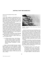
Introduction
As the world’s population and industrialization grow, air
pollution (Figure 1) becomes a progressively more serious
problem. The control of air pollution requires the involve-
ment of scientists from many disciplines: physics, chemistry
and mechanical engineering, meteorology, economics, and
politics. The amount of control necessary depends on the
results of medical and biological studies.
The state of the atmosphere affects, first, many types of pol-
lution. For example, on a cold day, more fuel is used for space
heating. Also, solar radiation, which is affected by cloudiness,
has an influence as smog production. Second, atmospheric
conditions determine the behavior of pollutants after they leave
the source or sources until they reach receptors, such as people,
animals, or plants. The question to be answered is: given the
meteorological conditions, and the characteristics of the source
or sources, what will be the concentration of the pollutants at
any distance from the sources? The inverse question also is
important for some applications: given a region of polluted air,
where does the pollution originate?
Finally, the effect of the pollution on the receptor may
depend on atmospheric conditions. For example, on a humid
day, sulfur dioxide is more corrosive than on a dry day.
Meteorological information is needed in three general
areas of air pollution control:
(1) In planning control measures, wind climatology
is required. Pollution usually must be reduced
to a point where the air quality is substantially

better than the existing quality. In order to assure
improved quality, certain standards are set which
prescribe maximum concentrations of certain
pollutants.
In order to reach such standards, the points of origin of
the pollution must first be located; traditionally, everybody
blames everybody else for the unsatisfactory air quality.
Given possible pollution sources, tracing of air trajectories
coupled with estimates of atmospheric dispersion will give
the required answers. Once the relative importance of differ-
ent pollution sources is known, strategies have to be devel-
oped to determine the degree to which each source must
reduce its effluent.
The most economical way to cut concentration of some
pollutant may not be to cut the effluent of each emitter by the
same amount. In order to find the best strategy, city models
must be constructed, separately for each pollutant and for
different meteorological conditions, which show how the air
pollution climate of an urban region is affected by the exist-
ing distribution of sources, and what change would be pro-
duced when certain sources are controlled. The construction
of such models will be discussed later, and requires a fairly
sophisticated handling of meteorological data. The same
models then also help in planning future growth of housing
and industry.
Of course, not all problems of air pollution meteorology
are as complex as those involving urban areas. The planning
of individual plants, for example, must be based in part on
the air pollution to be expected from the plant under various
atmospheric conditions; meteorological calculations may

show whether expensive techniques for cleaning the effluent
before leaving the stack may be required.
(2) Meteorological forecasts can be used to vary
the effluent from day to day, or even within a
24 hour period. This is because at different times
the atmosphere is able to disperse contaminants
much better than at other times; purer fuels must
be used, and operation of certain industries must
be stopped completely in certain areas when the
FIGURE 1 Air pollution in New York City prior to SO
2
and
particulate restriction.
© 2006 by Taylor & Francis Group, LLC
60 AIR POLLUTION METEOROLOGY
mixing ability of the atmosphere is particularly
bad.
(3) Meteorological factors have to be taken into
account when evaluating air pollution control
measures. For example, the air quality in a region
many improve over a number of years—not as
a result of abatement measures, but because of
gradual changes in the weather characteristics. If
the effects of the meteorological changes are not
evaluated, efforts at abatement will be relaxed,
with the result of unsupportable conditions when
the weather patterns change again.
Effects Between Source and Receptor
The way in which the atmospheric characteristics affect the
concentration of air pollutants after they leave the source can

be divided conveniently into three parts:
(1) The effect on the “effective” emission height.
(2) The effect on transport of the pollutants.
(3) The effect on the dispersion of the pollutants.
Rise of Effluent
To begin with the problem of effluent rise, inversion layers
limit the height and cause the effluent to spread out hori-
zontally; in unstable air, the effluent theoretically keeps
on rising indefinitely—in practice, until a stable layer is
reached. Also, wind reduces smoke rise.
There exist at least 40 formulae which relate the rise of
the meteorological and nonmeteorological variables. Most
are determined by fitting equations to smoke rise mea-
surements. Because many such formulae are based only
on limited ranges of the variables, they are not generally
valid. Also, most of the formulae contain dimensional con-
stants suggesting that not all relevant variables have been
included properly.
For a concise summary of the most commonly used
equations, the reader is referred to a paper by Briggs
(1969). In this summary, Briggs also describes a series of
smoke rise formulae based on dimensional analysis. These
have the advantage of a more physical foundation than the
purely empirical formulae, and appear to fit a wide range
of observed smoke plumes. For example, in neutrally stable
air, the theory predicts that the rise should be proportional to
horizontal distance to the 2/3 power which is in good agree-
ment with observations. The use of dimensionally correct
formulae has increased significantly since 1970.
Given the height of effluent rise above a stack, an

“effective” source is assumed for calculation of transport
and dispersion. This effective source is taken to be slightly
upwind of a point straight above the stack, by an amount
of the excess rise calculated. If the efflux velocity is small,
the excess rise may actually be negative at certain wind
velocities (downwash).
Transport of Pollutants
Pollutants travel with the wind. Hourly wind observations at
the ground are available at many places, particularly airports.
Unfortunately, such weather stations are normally several
hundred kilometers apart, and good wind data are lacking in
between. Further, wind information above 10 meters height
is even less plentiful, and pollutants travel with winds at
higher levels.
Because only the large-scale features of the wind pat-
terns are known, air pollution meteorologists have spent
considerable effort in studying the wind patterns between
weather stations. The branch of meteorology dealing with
this scale—the scale of several km to 100 km—is known as
mesometeorology. The wind patterns on this scale can be
quite complex, and are strongly influenced by surface char-
acteristics. Thus, for instance, hills, mountains, lakes, large
rivers, and cities cause characteristic wind patterns, both in
the vertical and horizontal. Many vary in time, for example,
from day to night. One of the important problems for the
air pollution meteorologist is to infer the local wind pattern
on the mesoscale from ordinary airport observations. Such
influences are aided by theories of sea breezes, mountain-
valley flow, etc.
In many areas, local wind studies have been made.

A particularly useful tool is the tetroon, a tetrahedral bal-
loon which drifts horizontally and is followed by radar. In
some important cities such as New York and Chicago, the
local wind features are well-known. In general, however, the
wind patterns on the mesoscale are understood qualitatively,
but not completely quantitatively. Much mesoscale numerical
modeling is in progress or has been completed.
Atmospheric Dispersion
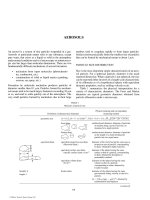
Dispersion of a contaminant in the atmosphere essentially
depends on two factors: on the mean wind speed, and on the
characteristics of atmospheric “turbulence.” To see the effect
of wind speed, consider a stack which emits one puff per
second. If the wind speed is 10 m/sec, the puffs will be 10 m
apart; if it is 5 m/sec, the distance is 5 m. Hence, the greater
the wind speed, the smaller the concentration.
Atmospheric “turbulence” consists of horizontal and
vertical eddies which are able to mix the contaminated air
with clean air surrounding it; hence, turbulence decreases the
concentration of contaminants in the plume, and increases
the concentration outside. The stronger the turbulence, the
more the pollutants are dispersed.
There are two mechanisms by which “eddies” are formed
in the atmosphere: heating from below and wind shear.
Heating produces convection. Convection occurs when-
ever the temperature decreases rapidly with height—that is,
whenever the lapse rate exceeds 1ЊC/100 m. It often pen-
etrates into regions where the lapse rate is less. In general,
convection occurs from the ground up to about a thousand
meters elevation on clear days and in cumulus-type clouds.
The other type of turbulence, mechanical turbulence,

occurs when the wind changes with height. Because there
© 2006 by Taylor & Francis Group, LLC
AIR POLLUTION METEOROLOGY 61
is no wind at ground level, and there usually is some wind
above the ground, mechanical turbulence just above the
ground is common. This type of turbulence increases with
increasing wind speed (at a given height) and is greater over
rough terrain than over smooth terrain. The terrain rough-
ness is usually characterized by a “roughness length” z
0
which varies from about 0.1 cm over smooth sand to a few
meters over cities. This quantity does not measure the actual
height of the roughness elements; rather it is proportional
to the size of the eddies that can exist among the roughness
elements. Thus, if the roughness elements are close together,
z
0
is relatively small.
The relative importance of heat convection and mechan-
ical turbulence is often characterized by the Richardson
number, Ri. Actually, – Ri is a measure of the relative rate
of production of convective and mechanical energy. For
example, negative Richardson numbers of large magnitude
indicate that convection predominates; in this situation, the
winds are weak, and there is strong vertical motion. Smoke
leaving a source spreads rapidly, both vertically and later-
ally (Figure 2).
As the mechanical turbulence increases, the
Richardson number approaches zero, and the angular disper-
sion decreases. Finally, as the Richardson number becomes

positive, the stratification becomes stable and damps the
mechanical turbulence. For Richardson numbers above 0.25
(strong inversions, weak winds), vertical mixing effectively
disappears, and only weak horizontal eddies remain.
Because the Richardson number plays such an important
role in the theory of atmospheric turbulence and dispersion,
Table 1 gives a qualitative summary of the implication of
Richardson numbers of various magnitudes.
It has been possible to describe the effect of roughness
length, wind speed, and Richardson number on many of the
statistical characteristics of the eddies near the ground quan-
titatively. In particular, the standard deviation of the vertical
wind direction is given by an equation of the form:
s
c
u
ϭ
Ϫ
fRi
ln z z Ri
()
()
.
/
0
(1)
Here z is height and f ( Ri ) and c( Ri ) are known functions
of the Richardson number which increase as the Richardson
number decreases. The standard deviation of vertical wind
direction plays an important role in air pollution, because it

determines the initial angular spread of a plume in the verti-
cal. If it is large, the pollution spreads rapidly in the vertical.
It turns out that under such conditions, the contaminant also
spreads rapidly sideways, so that the central concentrations
decrease rapidly downstream. If s
u
is small, there is negli-
gible spreading.
Equation 1 states that the standard deviation of vertical
wind direction does not explicitly depend on the wind speed,
but at a given height, depends only on terrain roughness and
Richardson number. Over rough terrain, vertical spreading is
faster than over smooth terrain. The variation with Richardson
number given in Eq. (1) gives the variation of spreading with
the type of turbulence as indicated in Table 1: greatest verti-
cal spreading with negative Ri with large numerical values,
less spreading in mechanical turbulence ( Ri ϭ 0), and negli-
gible spreading on stable temperature stratification with little
wind change in the vertical.
An equation similar to Eq. (1) governs the standard devi-
ation of horizontal wind direction. Generally, this is some-
what larger than s
u
. For light-wind, stable conditions, we do
not know how to estimate s
u
. Large s
u
are often observed,
particularly for Ri Ͼ 0.25. These cause volume meanders,

and are due to gravity waves or other large-sclae phenomena,
which are not related to the usual predictors.
In summary, then, dispersion of a plume from a continu-
ous elevated source in all directions increases with increasing
roughness, and with increasing convection relative to mechan-
ical turbulence. It would then be particularly strong on a clear
day, with a large lapse rate and a weak wind, particularly weak
in an inversion, and intermediate in mechanical turbulence
(strong wind).
a) Ri LARGE
CONVECTION
DOMINANT
b) Ri = 0
MECHANICAL
TURBULENCE
c) Ri > 0.25
NO VERTICAL
TURBULENCE
FIGURE 2 Average vertical spread of effluent from
an elevated source under different meteorological
conditions (schematic).
TABLE 1
Turbulence characteristics with various Richardson numbers
0.24 Ͻ Ri
No vertical mixing
0 Ͻ Ri Ͻ 0.25
Mechanical turbulence, weakened by
stratification
Ri ϭ 0
Mechanical turbulence only

Ϫ0.03 р Ri Ͻ 0
Mechanical turbulence and convection but
mixing mostly due to the former
Ri ϽϪ0.04
Convective mixing dominates mechanical
mixing
© 2006 by Taylor & Francis Group, LLC
62 AIR POLLUTION METEOROLOGY
Estimating Concentration of Contaminants
Given a source of contaminant and meteorological con-
ditions, what is the concentration some distance away?
Originally, this problem was attacked generally by attempt-
ing to solve the diffusion equation:
d
d
␹
tx
K
xy
K
yz
K
z
xyz
ϭ
Ѩ
Ѩ
Ѩ␹
Ѩ
ϩ

Ѩ
Ѩ
Ѩ␹
Ѩ
ϩ
Ѩ
Ѩ
Ѩ␹
Ѩ
.
(2)
Here, x is the concentration per unit volume; x, y, and z are
Cartesian coordinates, and the K ’s are diffusion coefficients,
not necessarily equal to each other.
If molecular motions produced the dispersion, the K ’s
would be essentially constant. In the atmosphere, where the
mixing is produced by eddies (molecular mixing is small
enough to be neglected), the K ’s vary in many ways. The diffu-
sion coefficients essentially measure the product of eddy size
and eddy velocity. Eddy size increases with height; so does
K. Eddy velocity varies with lapse rate, roughness length, and
wind speed; so does K. Worst of all, the eddies relevant to dis-
persion probably vary with plume width and depth, and there-
fore with distance from the source. Due to these complications,
solutions of Eq. (2) have not been very successful with atmo-
spheric problems except in some special cases such as continu-
ous line sources at the ground at right angles to the wind.
The more successful methods have been largely empiri-
cal: one assumes that the character of the geometrical distri-
bution of the effluent is known, and postulates that effluent is

conserved during the diffusion process (this can be modified
if there is decay or fall-out), or vertical spread above cities.
The usual assumption is that the distribution of effluent
from a continuous source has a normal (Gaussian) distribu-
tion relative to the center line both in the vertical direction, z
(measured from the ground) and the direction perpendicular
to the wind, y. The rationalization for this assumption is that
the distributions of observed contaminants are also nearly
normal.
†
Subject to the condition of continuity, the concen-
tration is given by (including reflection at the ground) .
x
pss
s
ss
ϭϪ
ϫϪϩ
Ϫϩ
Q
V
y
y
zHzH
yz
zz
2
2
22
2

2
2
2
2
exp
expexp
2
⎛
⎝
⎜
⎞
⎠
⎟
(
)
(
)
⎛
⎝

⎜⎜
⎞
⎠
⎟
.
(3)
Here, H is the “effective” height of the source, given by stack
height plus additional rise, σ is the standard deviation of the
distribution of concentration in the y and z -direction, respec-
tively, and V is the wind speed, assumed constant. Q is the

amount of contaminant emitted per unit time.
The various techniques currently in use differ in the way
s
y
and s
z
are determined. Clearly, these quantities change
with downwind distance x (Figure 3) as well as with rough-
ness and Richardson number.
Quantitative estimation of the Richardson number
requires quite sophisticated instrumentation; approximately,
the Richardson number can be estimated by the wind speed,
the time of the day and year, and the cloudiness. Thus, for
example, on a clear night with little wind, the Richardson
number would be large and positive, and s ’s in Eq. (3) are
small; on the other hand, with strong winds, the Richardson
numbers are near zero, and the dispersion rate as indicated
by the σ would be intermediate.
For many years, standard deviations were obtained by
Sutton’s technique, which is based on a very arbitrary selec-
tion for the mathematical form of Lagrangian correlation func-
tions. More popular at present is the Pasquill–Gifford method
in which s
y
and s
z
as function of x are determined by empirical
graphs (Figure 4). Note that the dependence of the standard
deviations on x varies with the “stability category” (from A
to F). These categories are essentially Richardson number cat-

egories, judged more or less subjectively. Thus, A (large dis-
persion) means little wind and strong convection; D is used
in strong winds, hence strong mechanical turbulence and less
dispersion; F applies at night in weak winds.
One drawback of the Pasquill–Gifford method is that it
does not allow for the effect of terrain roughness; the empiri-
cal curves were actually based on experiments over smooth
terrain, and therefore underestimate the dispersion over cities
and other rough regions. Some users of the method suggest
allowing for this by using a different system of categories
over rough terrain than originally recommended.
This difficulty can be avoided if fluctuations of wind
direction and vertical motion are measured. Taylor’s diffu-
sion theorem at right angles to the mean wind can be written
approximately,
ss
y
F
t
T
L
ϭϫ
0
⎛
⎝
⎜
⎞
⎠
⎟
.

(4)
Here F is a function which is 1 for small diffusion time, t. For
larger t, F decreases slowly; its behavior is fairly well known.
T
L
is a Lagrangian time scale which is also well known.
X
z
z
σ
σ
FIGURE 3 Change of vertical effluent
distribution downstream.
†
Note added in proof: It now appears that this assumption is not
satisfactory for vertical dispersion, especially if the source is near
the surface.
© 2006 by Taylor & Francis Group, LLC
AIR POLLUTION METEOROLOGY 63
10
2
10
2
10
3
10
4
10
1
10

3
10
4
4x10
0
10
5
2
2
5
5
2
5
2
5
10
2
10
3
3 x 10
3
10
1
10
0
2
2
5
2
2

5
5
2
5
2
5
σ
1
, HORIZONTAL DISPERSION COEFFICIENT (m)
σ
2
, VERTICAL DISPERSION COEFFICIENT (m)
DISTANCE FROM SOURCE (m)
A - EXTREMELY UNSTABLE
B - MODERATELY UNSTABLE
C - SLIGHTLY UNSTABLE
D - NEUTRAL
E - SLIGHTLY STABLE
F - MODERATELY STABLE
A
B
C
D
E
F
A - EXTREMELY UNSTABLE
B - MODERATELY UNSTABLE
C - SLIGHTLY UNSTABLE
D - NEUTRAL
E - SLIGHTLY STABLE

F - MODERATELY STABLE
A
B
C
D
E
F
FIGURE 4 Pasquill–Gifford scheme for estimating vertical and lateral plume
width as function of downwind distance and meteorological conditions.
© 2006 by Taylor & Francis Group, LLC
64 AIR POLLUTION METEOROLOGY
An equation similar to (4) also exists for vertical spread-
ing; however, it is theoretically less valid, since turbulence is
not homogeneous in the vertical.
As the plume expands vertically, the vertical distribution
cannot remain normal indefinitely. At the bottom, the plume
is limited by the ground. At the top, the plume will be lim-
ited by an elevated inversion layer. Eventually, the vertical
distribution becomes uniform. In that case, the concentration
is given by the equation:
x
Q
VD
y
y
y
ϭϪ
2
2
2

2
ps
s
exp (5)
where D is the height of the inversion layer, which is also
the thickness of the “mixed layer.” Note that the concentra-
tion is inversely proportional to VD, the “ventilation factor,”
which is the product of D, and V, the average wind in the
mixed layer.
The lateral spread is often limited by topography. In a
valley of width W, the factor
(2)()
22
expϪրրysps
yy
2
in
Eqs. (3) and (5) is replaced by 1/ W, after the contaminant
concentration fills the valley uniformly in the y -direction
(the direction perpendicular to the valley). The effect of this
change is that relatively large concentrations are maintained at
large distances from the sources.
Although the Pasquill–Gifford graphs are still popular
in practical applications, evaluation in diffusion experiments
have suggested serious deficiencies. Thus, the research com-
munity is groping for alternate methods. In particular, ver-
tical distributions are far from Gaussian, particularly for
ground sources. Significant progress has been made only for
the important case of light-wind, sunny conditions. Then, the
basic predictors are the thickness of the planetary boundary

layer (PBL), z
i
; another important predictor is a vertical-
velocity parameter, w
*
which is proportional to ( z
i
H)
1/3
where
H is the vertical heat flux at the surface. H is not usually mea-
sured, but must be estimated independently; fortunately, it is
raised to the 1/3 power. Lateral dispersion is still Gaussian,
but with s
y
given by
s
y
/ z
i
ϭ f( tw
*
/ z
i
)ϭ f( X ) where X ϭ tw
*
/ z
i
f is presumably universal and fairly well known.
The vertical distribution is definitely not Gaussian;

for example, the center line of the plume rises for ground
sources. More important, the center line comes down
toward the surface for elevated sources, unless the sources
are buoyant.
If vertical diffusion is normalized by the new variables,
it depends on z / z
i
, X and h / z
i
where h is stack height. The
distributions have been measured for different h / z
i
, and com-
plicated formulas exist to fit the observations. The results
are believed to be quite reliable, because numerical models,
laboratory experiments and full-scale observations are all in
satisfactory agreement.
The results of this research should be used in practi-
cal applications, but have not been. For more detail, see
Panofsky and Dutton, 1984.
City Models
These different methods give the pollutant concentrations
downwind from a single source. In order to obtain the total
picture of air pollution from a city, the concentrations result-
ing from all sources must be added together, separately for
all different wind directions, different meteorological condi-
tions, and for each contaminant. Such a procedure is expen-
sive, even if carried out with an electronic computer, and
even if, as is usually done, all small sources in square-mile
areas are combined. Therefore, complete city models of air

pollutant concentrations have only been constructed for very
few locations. It is necessary, however, to have city models
in order to understand the distribution of contaminants; only
then it is possible to determine the most economical strategy
to reduce the pollution, and to evaluate the effects of expan-
sion of housing and industry.
Because the construction of a complete city model is so
expensive, city models are often simplified. For example, if
the city is represented by a series of parallel line sources,
the computations are greatly reduced. Many other simplifi-
cations have been introduced; for a summary of many city
models now in existence, see Stern (1968).
Diurnal Variation of Air Pollution
Equation (5) which shows that concentrations at consider-
able distances from individual sources are inversely propor-
tional to the ventilation factor ( VD ), can be used to explain
some of the variations in air pollution caused by meteoro-
logical factors. First, we shall consider the diurnal variation
of air pollution. Of course, the actual variation of pollution
may be different if the source strength varies systematically
with time of day. The diurnal variation is different in cities
and in the country. Consider typical vertical temperature
distributions as seen in Figure 5. During the day, both over
cities and country, the ground temperature is high, giving a
deep mixed layer. After sunset, the air temperature near the
surface in the country falls, producing an inversion reaching
down to the ground. After air moves from the country out
over the relatively warmer and rougher city, a thin mixed
layer is formed near the ground. The thickness of this mixed
10,000

5,000
COUNTRY
CITY
CITY
COUNTRY
NIGHT
DAY
TEMPERATURE
HEIGHT, ft
FIGURE 5 Vertical temperature distribution
(schematic) over city and country, day and night.
© 2006 by Taylor & Francis Group, LLC
AIR POLLUTION METEOROLOGY 65
layer varies with the size of the city, and depends on how
long the air has moved over the city. In New York, for exam-
ple, the mixed layer is typically 300 m thick; in Johnstown,
Pa., an industrial valley city with just under 100,000 popu-
lation, it is only a little over 100 m.
Figure 6 indicates how the temperature changes shown
in Figure 5 influence the diurnal variation of pollution due
to an elevated source in the country; at night, vertical mixing
is negligible and the air near the ground is clean. Some time
shortly after sunrise, the mixed layer extends to just above
the source, and the elevated polluted layer is mixed with the
ground air, leading to strong pollution (also referred to as
“fumigation”), which may extend many kilometers away
from the source. Later in the morning and early afternoon,
the heating continues and thickens the mixed layer. Also, the
wind speed typically increases, and the pollution decreases.
In the city, many sources usually exist in the thin night-

time mixed layer. Since this layer is so thin, and the wind
usually weak, dense pollution occurs at night. Right after
sunrise, the pollution at first increases somewhat, as the efflu-
ent from large, elevated sources is brought to the ground. As
the mixed layer grows, the concentrations diminish, and, in
the early afternoon, they are often less than the nighttime
concentrations (see Figure 7).
Thus, the main difference between air pollution climates
in the city and country is that country air near industrial
sources is usually clean at night, whereas the city air is dirtier
at night than in the middle of the day. These differences are
most pronounced during clear nights and days, and can be
obliterated by diurnal variations of source strengths. Figure 7
shows the characteristic behavior only because the sources of
pollution at Johnstown, Pa., are fairly constant throughout.
MIDDAY
DAY
MORNING (FUMIGATION)
MORNING (FUMIGATION)
NIGHT
NIGHT
COUNTRY
CITY
MIXED LAYER
FIGURE 6 Concentrations of effluent (schematic) as function of time of day, over
city and country.
50
40
30
20

05101520
Time of day
100-T, (%)
FIGURE 7 Concentrations of air pollution (100-T%), as function of time of day, on clear
day (solid line) and cloudy day (dashed line), at Johnstown, Pa.
© 2006 by Taylor & Francis Group, LLC
66 AIR POLLUTION METEOROLOGY
Day-to-day Variations in Air Pollution
Equation (5) shows that, other things being equal, the con-
centration of contaminants is inversely proportional to the
wind speed. Figure 8 shows this effect on 24-hr total particu-
late concentration at Johnstown, for cases where the source
strengths were roughly the same, during the fall of 1964.
Conditions of particularly bad air pollution over wide
areas and for extended periods are accompanied not only by
light winds and calms, but also by unusually small mixing
depths ( D ) so that the ventilation factor is usually small.
Such conditions occur within large high-pressure areas
(anticyclones). In such areas, air is sinking. Sinking air is
warmed by compression. Thus, in an anticyclone (high-pres-
sure area), an elevated warm layer forms, below which there
is room only for a relatively thin mixed layer (Figure 9).
The
inversion on top of the mixed layer prevents upward spread-
ing of the pollution, and when mountains or hills prevent
sideways spreading the worst possible conditions prevail.
A particularly bad situation arose in the industrial valley
town of Donora, Pa., in which many people were killed by
air pollution in 1948.
Cities in California, like Los Angeles, are under the influ-

ence of a large-scale anticyclone throughout the summer, and
an elevated inversion at a few hundred meters height occurs
there every day; that is why Los Angeles had air pollution
problems as soon as pollutants were put into the atmosphere
to any large extent. In the United States outside the West
Coast, stagnant anticyclones occur only a few times per year,
usually in the fall.
So far, relatively little use has been made in the USA of
forecast changes in air pollution potential from day to day.
As air pollution problems become more severe, more use
will be made of such forecasts. Already, this type of infor-
mation has proved itself in air pollution management in
some European countries.
Not much has been said about the influence of wind
direction on air pollution. When pollution is mainly due to
many, relatively small sources, as it is New York, the pollu-
tion is surprisingly insensitive to changes in wind direction.
Even in Johnstown, Pa., wind direction is unimportant except
for the case of easterly winds, when a single, huge steel plant
adds significantly to the contaminant concentration.
In contrast, wind direction plays a major role when most
of the pollution in a given area is due to a single or a few
major plants or if an industrial city is nearby. Also, there
are special situations, in which wind direction is particularly
important; for example, in Chicago, which has no pollution
sources east of the city, east winds bring clean air.
The main difference between the effects of lapse rate,
mixing depth, and wind speed on the one hand, and wind
R
R

500
400
300
200
100
0
01
2
34 56
7
8
9
10
CONCENTRATION, g/m
3
Viso. mph
µ
FIGURE 8 Dependence of 24-hour average particle concentrations at Johnstown on wind speed at 150 ft.
R denotes rain.
BEFORE
SINKING
AFTER
SINKING
INVERSION
LAYER
MIXED
LAYER
D
T
Z

FIGURE 9 Effect of sinking on vertical temperature
distribution (schematic).
© 2006 by Taylor & Francis Group, LLC
AIR POLLUTION METEOROLOGY 67
direction on the other, is that the wind direction has different
effects at various sites, depending on the location of the
sources; the other factors have similar effects generally.
EFFECT OF AIR POLLUTION ON LOCAL
AND REGIONAL WEATHER
Visibility
The most obvious effect of air pollution is to reduce vis-
ibility. This effect has been studied frequently by comparing
visibility in different parts of a city, or the visibility in a city
with visibility in the country. For a summary of many such
investigations, see Peterson, 1969.
To give some examples: Around London and
Manchester, afternoon visibility less than 6
1
ր
4
miles occurs on
more than 200 days; in Cornwall in SW England, the number
is less than 100. In central London, there are 940 hours a year
with visibilities less than
5
ր
8
mile; in SE England, only 494.
In many cities, visibilities have recently improved prob-
ably due to control of particle emissions; however, as men-

tioned before, some of this change may be due to changes in
large-scale weather patterns.
Although decreased visibility is usually associated
with industrial or automobile pollution, considerable atten-
tion has been paid recently to decreased visibilities due to
the “contamination” of the atmosphere by water droplets
by industry. This problem arises because many processes
generate excess heat; if this is added to streams and lakes,
undesirable effects ensue; hence, progressively more and
more heat is used to evaporate water which is then emit-
ted into the atmosphere, and later condenses to form water
plumes.
There are many unpublished studies estimating the
effect of cooling towers on visibility. This varies greatly
with meteorological conditions, but is particularly serious in
winter, then the air is nearly saturated and little additional
vapor is required to produce liquid drops. Under those con-
ditions, water plumes from industries produce clouds and
fog which may reach over a hundred miles from the sources.
Automobile accidents have been blamed on such fogs, par-
ticularly when the particles freeze and make roads slippery,
adding to the visibility hazard.
Sunshine Intensity
“Turbidity” is an indicator of the reduction of light due to
haze, smoke and other particles. Turbidity is now being
monitored at many places in the world. It is quite clear that
it is larger over cities than over the country; it has been sug-
gested that the average decrease of sunshine over cities is
15 to 20% due to pollution. The effect is even larger if only
ultraviolet light is considered.

Control of smoke emission in cities such as London has
caused a very noticeable increase of sunshine intensity: for
example the hours of “Bright sunshine” increased by 50%
after control measures had become effective. Again, for a
summary of some of these studies, the reader is referred to
Peterson, 1969.
Precipitation Amount
There have now been several studies suggesting that pre-
cipitation is increased downstream of industrial centers.
The investigations are of a statistical nature, and it is not
known whether the effects are due to increased convection
(increased heat), increased condensation nuclei or increased
water vapor. Further, the reliability of the statistics has been
questioned.
For example, Changnon (1969) found a large precipita-
tion anomaly at La Porte (Indiana) just downwind of large
industrial complexes of Northwestern Indiana. But change in
observational techniques of rainfall and other uncertainties
have thrown doubt on the results. Hobbs et al. (1970) have
compared rainfall distribution in Western Washington before
and after the construction of industries and found an increase
by 30% or so; but some of this increase may have been due
to “normal” climatic change. For a summary of these and
other studies see Robinson (1970). It becomes quite clear
from this summary that more, careful investigations of this
type are needed before effects of air pollution on precipita-
tion patterns can be definitely proven.
A large study (Metromex) found strong enhancement of
precipitation downwind of St Louis. But this may be due to
the St Louis heat sources rather than to pollution.

Acid Rain
There is no question that acid rain is produced by atmospheric
pollution. The acidity of rainfall is large only when the wind
direction suggests industrial or urban sources. Most impor-
tant is sulphuric acid, produced by power plants or smelt-
ers, the effluent from which contains SO
2
. Also important is
nitric acid, which is formed mostly from nitrogen oxides in
car exhausts. Acid rain has done important damage to lakes
and forests; but there is controversy how to deal with the
problem. For example, the relation between acidity and SO
2
may be nonlinear, so that substantial reduction of SO
2
may
not effect acid rain significantly.
GLOBAL EFFECTS OF AIR POLLUTION
Natural Climatic Changes
We will assess the effect of some atmospheric pollutants as
to their ability to change the earth’s climate. In doing so,
we are hampered by the fact that the present climate is pro-
duced by a multitude of interacting factors; if one factor is
changed, others will too, and a complex chain reaction will
ensue. These reactions can be studied by complex math-
ematical models of the atmosphere, which so far have been
quite successful in describing the existing climate. But, as
yet these models contain assumptions which make it impos-
sible at this time to assess accurately the effects of changes
© 2006 by Taylor & Francis Group, LLC

68 AIR POLLUTION METEOROLOGY
in some of the factors affecting climate. Until such models
are improved, then, we cannot really estimate quantitatively
climatic changes produced by pollutants.
The concentration of CO
2
is about 340 parts per million
(ppm). According to observations at Mauna Loa in Hawaii,
over the last forty years or so, it has increased at the rate of
0.7% per year. This is less than half the amount put into the
atmosphere by industry. The other half goes into the ocean
or into vegetation; but it is not known how much goes into
each. Further, we do not know whether the same fraction
can disappear out of the atmosphere in the future—e.g., the
amount going into the ocean is sensitive to temperature, and
the amount going into vegetation may be limited by other fac-
tors. However, a reasonable guess is that the fraction of CO
2
in
the atmosphere will double in the middle of the 21st century.
The basic effect of CO
2
on climate is due to the fact that
it transmits short-wave radiation from the sun, but stops a part
of the infrared radiation emitted by the earth. Hence, the more
CO
2
, the greater the surface temperature. This is known as the
greenhouse effect. Also, since CO
2

increases the radiation into
space, the high atmosphere is cooled by increasing CO
2
.
The heating rate at the ground expected with a doubling
of CO
2
has been calculated by many radiation specialists.
The answers differ, depending on how many other vari-
ables (such as cloud cover) are allowed to change as the
CO
2
changes. The best current estimates are that doubling
CO
2
would increase the surface temperature about 2ЊC, and
decrease the temperature aloft a little more. But these esti-
mates do not treat changes of cloud cover and oceanic effects
realistically, and these estimates may yet be corrected. Still,
if we expect only a 20% change in CO
2
by the end of the cen-
tury, the climatic change due to this factor should be small.
However, a serious problem could arise in the next century,
particularly because it is difficult to see how a trend in CO
2
concentration can be reversed. It is therefore of great impor-
tance to continue monitoring CO
2
concentration accurately.

As of 1987, it appears likely that increases of concentra-
tion of other trace gases (e.g. fluorocarbons) may, in combi-
nation, have as strong a warming effect at the surface as CO
2
.
So far, no significant warming has been detected.
Ozone
Ozone (O
3
) is an important part of photochemical smog;
originating mostly from the effect of sunlight on automobile
exhaust. The concentration is critically dependent on chemi-
cal reactions as well as on diffusion. Chemistry is beyond
the scope of this paper as O
3
and ozone pollution near the
ground will not be discussed further.
More important, 90% of the ozone exists in the strato-
sphere (above about 11 km). Its concentration even there is
small (usually less than 10 ppm). If all ozone were to be
brought to the surface of the ground, its thickness would
average about 0.3 cm.
Most of the ozone occurs at high latitudes, and there is
a spring maximum. The great importance of stratospheric
ozone is due to its ability to absorb ultraviolet (UV) light,
particularly in the UVB region (290–320 µ m) where human
skin is extremely sensitive. Thus, decreased ozone would
increase skin cancer.
We now realize that small fractions (10
−9

) of certain
gases can destroy ozone by catalytic reactions. The most
important are oxides of nitrogen and chlorine. Nitrogen
oxides could originate for example, from supersonic trans-
ports. However calculations show that, unless the number of
SSTs is increased significantly, this problem is not serious.
More important is the problem of chlorofluorometh-
anes (CFM) the use of which has been rapidly increasing.
They are used in sprays, foams and refrigeration, CFMs
are so stable that most of them are still in the atmosphere.
Eventually, however, CFMs will seep into the stratosphere
(about 1%/year). In the high stratosphere, UV will dissociate
CFMs producing chlorine, which destroys ozone.
A slow decrease of ozone in the stratosphere has indeed
been indicated by recent satellite observations. For total
ozone, the results are much more controversial. Chemical–
meterological models show only a very small decrease so far,
too small to isolate from the “noisy” observations. However,
the accuracy of the models can be questioned, particularly
since new relevant reactions have been discovered every few
years, so that model results have varied.
Of special interest has been the recognition of an “ozone
hole,” centered at the South Pole, and lasting a month or so
in the Southern Spring. Total column ozone falls to about
half its normal value. The phasing out of chlorofluorocar-
bons, or CFCs began in 1989 with the implementation of the
Montreal Protocol.
Editors Notes: Scientists at NASA and various U.S.
universities have been studying satellite data taken over the
past 2 decades. They found the rate of ozone depletion in the

upper stratosphere is slowing partially as a result of a reduc-
tion in the use of CFCs (see Newchurch, et al., 2005).
In the troposphere, aerosol formation from the combus-
tion of fossil fuels and biomass is a precursor to the forma-
tion of brown clouds, which are intricately linked to climate
changes (Ramanathan and Ramana, 2003). Ozone, a com-
ponent of smog, also forms in the troposphere, when NO
x
combines with volatile organic compounds in the presence of
sunlight. There is growing scientific evidence that the inter-
continental transport (ICT) of aerosols and ozone influences
surface air quality over downwind continents (Fiore, et al.,
2003). For example during the dust storm events in Asia in
April of 2001, the ground level aerosol concentrations in the
western U.S. and Canada increased by as much as 40 µ g/m
3
resulting from the ICT of aerosols. Fiore, et al. found there
are global dimensions to the aerosol and ozone problems.
It has also been suggested that ozone changes can pro-
duce climate changes, but these appear rather unimportant at
present, except that they may worsen slightly the CO
2
green-
house effect.
Summary
In summary, increasing air pollution can modify the climate in
many ways. There is no evidence that any significant change
has occurred so far; but eventually, large effects are likely.
© 2006 by Taylor & Francis Group, LLC
AIR POLLUTION METEOROLOGY 69

REFERENCES
1. Briggs, G.A. (1969), Plume Rise. USAEC critical review series, TID-
25075, Clearinghouse for federal scientific and technical information.
2. Changnon, S.H. (1968), The LaPorte Weather Anomaly, fact or fiction,
Bull. Amer. Met. Soc., 49, pp. 4–11.
3. Fiore, A.T. Holloway and M. Galanter, Environmental Manager,
pp. 13–22, Dec. 2003.
4. Hanna, S.R., G. Briggs, J. Deardorff, B.E. Egan, F.A. Gilfford, and
F. Pasquill (1977), AMS workshop on stability classification schemes
and sigma curves, Bull. Amer. Met. Soc., 58, pp. 1305–1309.
5. Hobbs, P.V., L.F. Radke, and S.E. Shumway (1970), Cloud conden-
sation nuclei from industrial sources and their apparent influence on
precipitation in Washington State, Jour. Atmos. Sci., 27, pp. 81–89.
6. Newchurch, M.J., Journal of Geophysical Research, V110, 2005.
7. Panofsky, H.A. and F.X. Dutton (1984), Jour. Atmos. Sci., 41, pp. 18–26.
8. Peterson, J.T. (1969), The Climate of Cities: A Survey of Recent
Literature. US Dept. HEW, NAPCA, Pub. No. AP-50.
9. Ramanathan, V. and M.V. Ramana, Environmental Manager, pp. 28–33,
Dec. 2003.
10. Robinson, G.D. (1970), Long-Term Effects of Air Pollution, Center for
Environment and Man, Hartford, CEM 4029–400.
11. Schoeberl, M.A. and A.J. Krueger (1986), Geoph. Res. Paper ’ s Suppl.
13, No. 12.
12. Stern, A.C. (1976), Air Pollution, Vol. 1, Academic Press, New York.
3rd Ed.
HANS A. PANOFSKY (DECEASED)
Pennsylvania State University
AIR POLLUTION MODELING — URBAN: see URBAN
AIR POLLUTION MODELING
© 2006 by Taylor & Francis Group, LLC