ENCYCLOPEDIA OF ENVIRONMENTAL SCIENCE AND ENGINEERING - NOISE pptx

769
NOISE
Noise and sound refer to audible pressure fluctuations in air.
Both are characterized by sound level in decibels and fre-
quency content in hertz. Although sound is vital for commu-
nication, noise is one of our greatest problems. Intentionally
generated acoustic signals including speech and music are
usually referred to as sound. Noise is a term used to identify
unwanted sound, including sound generated as a byproduct
of other activities such as transportation and industrial opera-
tions. Intrusive sound, including speech and music unwelcome
to the hearer, are also considered noise. Thus, the distinction
between noise and sound is subjective, and the two terms are
often used interchangeably.
When a body moves through a medium or vibrates, some
energy is transferred to that surrounding medium in the form
of sound waves. Sound is also produced by turbulence in air
and other fluids, and by fluids moving past stationary bodies.
In general, gases, solids and liquids transmit sound.
Well-documented effects of noise include hearing
damage, interference with communication, masking of
warning signals, sleep interruption, and annoyance. Noise
detracts from the quality of life and the environment; it con-
tributes to anger and frustration and has been implicated as a
contributor to psychological and physiological problems.
The National Institute for Occupational Safety and
Health (NIOSH) named hearing loss as a priority research
area, noting that noise-induced hearing loss is 100% prevent-
able, but once acquired, it is permanent and irreversible. The
Occupational Safety and Health Administration (OSHA)
noted that hearing loss can result in a serious disability, and

put employees at risk of being injured on the job. The World
Health Organization (WHO) notes that noise-induced hearing
impairment is the most prevalent irreversible occupational
hazard, and estimates that 120 million people worldwide
have disabling hearing difficulties. In developing countries,
not only occupational noise but also environmental noise is
an increasing risk factor for hearing impairment.
The European Union (EU) identified environmental
noise caused by traffic, industrial and recreational activities
as one of the main local environmental problems in Europe
and the source of an increasing number of complaints. It is
estimated that 20% of the EU population suffer from noise
levels that both scientists and health experts consider unac-
ceptable. An additional 43% of the population live in ‘gray
areas’ where noise levels cause serious daytime annoyance.
Estimates of the cost of noise to society range from 0.2% to
2% of gross domestic product.
Noise control involves reduction of noise at the source,
control of noise transmission paths, and protection of the
receiver. Source control is preferred. For example, design of
transportation systems and machinery for lower noise output
may be the most effective means of noise control. But, after
trying all feasible noise source reduction, airborne noise and/
or solid-borne noise may still be objectionable. Interruption
of noise transmission paths by means of vibration isolation,
source enclosures, sound absorbing materials, or noise barri-
ers is then considered.
In some industrial situations, excessive noise is still pres-
ent after all attempts to control noise sources and transmission
paths. Administrative controls—the assignment of employees

so that noise exposure in reduced—should then be consid-
ered. As a last resort, employees may be required to use per-
sonal hearing protection devices (muff-type and insert-type
hearing protectors). Communities often resort to ordinances
that limit noise levels and restrict hours of operation of noise-
producing equipment and activities. Community noise con-
trol methods also include zoning designed to separate noise
sources from residential and other sensitive land uses.
FREQUENCY, WAVELENGTH AND PROPAGATION
SPEED
Frequency. Audible sound consists of pressure waves with
frequencies ranging from about 20 hertz (Hz) to 20,000 Hz,
where 1 Hz ϭ 1 cycle per second. Sound consisting essen-
tially of a single-frequency sinusoidal pressure wave is called
a pure tone. In most cases, noise consists of sound waves
arriving simultaneously from a number of sources, and
having a wide range of frequencies. A sound wave which has
a frequency below the audible range is called infrasound
and sound of frequency above the audible range is called
ultrasound.
Propagation speed. The propagation speed of airborne
sound is temperature dependent. It is given by:
c ϭ 20.04[TЈ ϩ 273.16]
1/2
(1.1)
where c ϭ propagation speed, i.e. the speed of sound, (m/s)
T Ј ϭ air temperature (ЊC).
At an air temperature of T Ј ϭ 20ЊC (68ЊF), the propaga-
tion speed is c ϭ 343 m/s (approx). Sound waves propagate
at a different speed in solids and liquids. The propagation

speed for axial waves in a steel rod is about 5140 m/s. Note that
C014_003_r03.indd 769C014_003_r03.indd 769 11/18/2005 10:46:06 AM11/18/2005 10:46:06 AM
© 2006 by Taylor & Francis Group, LLC
770 NOISE
c is a wave a propagation speed; it does not represent particle
velocity within the medium.
Wavelength. If a pure-tone pressure wave could be
observed at a given instant, the length of one cycle of the
wave in the propagation directly could be identified as the
wavelength. Thus,
λ ϭ c / f (1.2)
where λ ϭ wavelength (m), c ϭ propagation speed (m/s) and
f ϭ frequency (Hz). The effectiveness of noise barriers and
sound-absorbing materials is dependent on the sound wave-
length (thus, effectiveness is frequency-dependent).
SOUND PRESSURE AND SOUND PRESSURE LEVEL
One standard atmosphere is defined as a pressure of 1.01325 ϫ
10
5
Pa (about 14.7 psi). Typical sound pressure waves rep-
resent very small disturbances in ambient pressure. Sound
pressure level is defined by


Lpp pp
pgrms
2
ref
2
rms ref

lgϭϭ10 20 1⁄
⎡
⎣
⎤
⎦
[]
ր

(2.1)

where L
p
ϭ sound pressure level in decibels (dB), lg ϭ
common (base-ten) logarithm, p
rms
ϭ root-mean-square sound
pressure (Pa) and p
ref
ϭ reference pressure ϭ 20 ϫ 10
−6
Pa.
Sound pressure represents the difference between instan-
taneous absolute pressure and ambient pressure. For a pure-
tone sound wave of amplitude P ,
p
rms
ϭ P /2
1/2
.
The reference pressure is the nominal threshold of hearing,

corresponding to zero dB. Sound pressure may be determined
from sound pressure level by the following relationship:


pp
L
L
rms ref
p
P
ϭϫ ϭϫ
Ϫ
10 2 10
20
100 20
⁄
[]
⁄ .

(2.2)

A-WEIGHTING
Human hearing is frequency-dependent. At low sound levels,
sounds with frequencies in the range from about 1 kHz to
5 kHz are perceived as louder than sounds of the same sound
pressure, but with frequencies outside of that range. A-, B-
and C-weighting schemes were developed to compensate for
the frequency-dependence of human hearing at low, moder-
ate and high sound levels. Other weightings are also used,
including SI-weighting which relates to speech interference.

A-weighting has gained the greatest acceptance; many stan-
dards and codes are based on sound levels in A-weighted
decibels (dBA). When noise is measured in frequency bands,
the weighting adjustment may be added to each measured
value. Sound level meters incorporate weighting networks
so that weighted sound level is displayed directly. A-weight-
ing adjustments are shown in Table 1.
Some representati
Most values are approximate; actual noise sources produce a
wide range of sound levels.
EQUIVALENT SOUND LEVEL
Sound energy is proportional to mean-square sound pressure.
Equivalent sound level is the energy-average A-weighted
sound level over a specified time period. Thus,


LTt
L
T
eq
lg dϭ10 1 10
10
0
⁄
(
)
⎡
⎣
⎢
⎤

⎦
⎥
⁄
∫

(4.1)

where L
eq
ϭ equivalent sound level (dBA), L ϭ instantaneous
sound level (dBA) and T ϭ averaging time, often 1 hour, 8
TABLE 1
A-weighting
Frequency
Hz
Adjustment
dB
20 Ϫ50.5
25 Ϫ44.7
31.5 Ϫ39.4
40 Ϫ34.6
50 Ϫ30.2
63 Ϫ26.2
80 Ϫ22.5
100 Ϫ19.1
125 Ϫ16.1
160 Ϫ13.4
200 Ϫ10.9
250 Ϫ8.6
315 Ϫ6.6

400 Ϫ4.8
500 Ϫ3.2
630 Ϫ1.9
800 Ϫ0.8
1,000 0
1,250 ϩ0.6
1,600 ϩ1.0
2,000 ϩ1.2
2,500 ϩ1.3
3,150 ϩ1.2
4,000 ϩ1.0
5,000 ϩ0.5
6,300 Ϫ0.1
8,000 Ϫ1.1
10,000 Ϫ2.5
12,500 Ϫ4.3
16,000 Ϫ6.6
20,000 Ϫ9.3
C014_003_r03.indd 770C014_003_r03.indd 770 11/18/2005 10:46:07 AM11/18/2005 10:46:07 AM
© 2006 by Taylor & Francis Group, LLC
ve sound levels are given in Table 2.
NOISE 771
hours, 24 hours, etc. The time period may be identified by the
subscript, e.g. L
eq24
for a 24 hour averaging time.
Integrating sound level meters compute and display
equivalent sound level directly. If equivalent sound level is
to be determined from a number of representative instanta-
neous measurements or predictions, the above equation may

be rewritten as follows:


LN
L
i
N
eq
lgϭ10 1 10
10
1
⁄
(
)
⎡
⎣
⎢
⎤
⎦
⎥
⁄
=
∑
i
.

(4.2)

If a large number of readings are involved, it is con-
venient to incorporate the above equation into a computer

program. If the base-10 logarithm is not available on the
computer it may be obtained from



lg n n 10xx
(
)
(
)
⁄
(
)
ϭ11

(4.3)

where ln is the natural (base-e) logarithm.
Example Problem: Equivalent Sound Level
Considering four consecutive 15-minute intervals, during
which representative sound levels are 55, 58, 56 and 70 dBA
respectively. Determine equivalent sound level for that hour.
Solution:

L
eq
lg 1 4
dBA.
ϭϩϩϩ
ϭ

10 10 10 10 10
64 5
55 10 58 10 56 10 70 10
⁄
(
)
()
⁄⁄⁄⁄
.


It can be seen that higher sound levels tend to dominate when
determining L
eq
. Note that the mean average sound level (55 ϩ
58 ϩ 56 ϩ 70)/4 ϭ 59.8 has no significance.
DAY–NIGHT SOUND LEVEL
Day–night sound level takes into account the importance of
quiet during nighttime hours by adding a 10 dBA weighting
to noise during the period from 10 pm to 7 am. It is given by


Lt
t
L
L
DN
am
pm
pm

am
lg 1/24 dϭϩ
ϩ
10 10
10
10
7
10
10
7
[]
⎡
⎣
⎢
{
⎤
⎦
⁄
∫
∫
( 10) 10ր
d
⎥⎥
}
(5.1)
where L
DN
ϭ day–night sound level and t ϭ time (hours).
COMBINING NOISE FROM SEVERAL SOURCES
Correlated sound waves. Sound waves with a precise time

and frequency relationship may be considered correlated.
A sound wave arriving directly from a source may have a
precise phase relationship with a reflected sound wave from
the same source. The sound level resulting from combining
two correlated sound waves of the same frequency depends
on the phase relationship between the waves. Reactive muf-
flers and silencers are designed to produce reflections that
cancel the progressive sound wave.
Active noise control is accomplished by generating
sound waves out-of-phase with the noise which is to be
cancelled. Active noise control systems employ continuous
measurement, signal processing, and sound generation.
Uncorrelated noise sources. Most noise sources are not
correlated with one another. The combined effect of two or
more uncorrelated sources is obtained by combining the energy
from each at the receiver. To do this, we may add mean-square
sound pressures. In terms of sound levels, the result is


L
L
i
N
i
T
=
⁄
=
∑
10 10

10
1
lg

(6.1)

where L
T
ϭ total sound level due to N contributions L
i
(dBA
as measured or predicted at the receiver).
For two contributions, the total sound level is



L
L
LL
T
DIF 10
lg 10
lg 1 10
ϭϩ
ϭϩ ϩ
Ϫ
10 10
10
110 210
1

⁄⁄
⁄
⎡
⎣
⎤
⎦
⎡
⎣
⎤
⎦
(6.2)
where L
1
ϭ the greater sound level and DIF ϭ L
1
Ϫ L
2
, the
difference between the two sound levels.
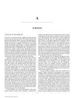
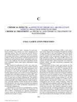
The last term in equation 6.2 may be identified as L (add), the
quantity to be added to L
1
to obtain total sound level L
T
. L (add)
Values are given to the nearest one-tenth decibel. Although
measured and predicted sound levels are often reported to the
TABLE 2
A-weighted sound levels
Approximate

sound level Noise source or criterion
140 Threshold of pain
122 Supersonic aircraft
A
120 Threshold of discomfort
112 Stage I aircraft
A
110 Leaf blower at operator
105 OSHA 1 hr/da limit
B
99 EEC 1 hr/da limit
B
90 OSHA and EEC 8 hr/da limit
B
70 EPA criterion for hearing conservation
C
67 DOT worst hour limit
D
65 Daytime limit, typical community ordinance
45 Noise limit for virtually 100% indoor speech intelligibility
35 Acceptable for sleep
0 Threshold of hearing
Notes:
A: Aircraft measurements 500 ft beyond end of runway, 250 ft to side.
Stage 3 aircraft in current use are quieter.
B: Criteria for worker exposure (US Occupational Safety and Health
Administration and European Economic Community).
C: Environmental Protection Agency identified 24-hr equivalent sound level.
D: Department of Transportation design noise level for residential use.
C014_003_r03.indd 771C014_003_r03.indd 771 11/18/2005 10:46:07 AM11/18/2005 10:46:07 AM

© 2006 by Taylor & Francis Group, LLC
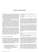
is tabulated against DIF, the difference in levels, in Table 3.
772 NOISE
nearest whole decibel, fractional values are often retained for
comparison purposes, and to insure accuracy of intermediate
calculations.
Note that addition of the contributions of two equal but
uncorrelated sources produces a total sound level 3 decibels
higher than the contribution of one source alone.
If the difference between contributions is 10 or more
decibels, then the smaller contribution increases total sound
level by less than one-half decibel. If the difference is 20
or more decibels, the smaller contribution has no significant
effect; for DIF Ն 20, L (add)Ͻ 1/20. This is an important
consideration when evaluating noise control efforts. If sev-
eral individual contributions to overall sound level can be
identified, the sources producing the highest sound levels
effect of combining noise levels.
Example Problem: Combining Noise Contributions
The individual contributions of five machines are as follows
when measured at a given location: 85, 88, 80, 70 and 95 dBA.
Find the sound level when all five are operating together.
Solution:
Using equation 6.1, the result is L
T
ϭ 10 lg[10
85/10
ϩ
10
88/10

ϩ 10
80/10
ϩ 10
70/10
ϩ 10
95/10
] ϭ 96.25 dBA. We could
use Table 3 instead. Combining the levels in ascending order,
the result is
70 ϩ 80 ϭ 80.4 and
80.4 ϩ 85 ϭ 86.3 and
86.3 ϩ 88 ϭ 90.3 and
90.3 ϩ 95 ϭ 96.3 dBA
Fractional parts of one dBA are only retained for purposes
or illustration.
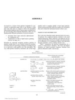
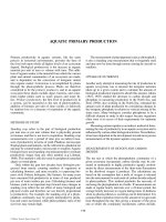
For several sources which contribute equally to sound
level at the receiver, total sound level is given by


LL n
T
ϭϩ
1
10 lg
(6.3)
where L
1
ϭ sound level contribution at the receiver due to
a single source and n ϭ the number of sources. Table 3 and
related) contributions.

SOUND FIELDS
The region within one or two wavelengths of a noise source
or within one or two typical source dimensions is called the
near field. The region where reflected sound waves have a
significant effect on total sound level is called the reverber-
ant field. Consider an ideal nondirectional noise source which
generates a spherical wave. For regions between the near field
and the reverberant field, sound intensity is given by


IW rϭ ⁄
⎡
⎣
⎤
⎦
4
2
p

(7.1)

TABLE 3
Combining noise from two uncorrelated sources
DIF L(add) DIF L(add)
0.0 3.0 5.0 1.2
0.2 2.9 5.5 1.1
0.4 2.8 6.0 1.0
0.6 2.7 6.5 0.9
0.8 2.6 7.0 0.8
1.0 2.5 7.5 0.7

1.2 2.5 8.0 0.6
1.4 2.4 8.5 0.6
1.6 2.3 9.0 0.5
1.8 2.2 9.5 0.5
2.0 2.1 10.0 0.4
2.2 2.0 10.5 0.4
2.4 2.0 11.0 0.3
2.6 1.9 11.5 0.3
2.8 1.8 12.0 0.3
3.0 1.8 12.5 0.2
3.2 1.7 13.0 0.2
3.4 1.6 13.5 0.2
3.6 1.6 14.0 0.2
3.8 1.5 14.5 0.2
4.0 1.5 15.0 0.1
4.2 1.4 15.5 0.1
4.4 1.3 16.0 0.1
4.6 1.3 16.5 0.1
4.8 1.2 17.0 0.1
— — 17.5 0.1
— — 18.0 0.1
— — 18.5 0.1
— — 19.0 0.1
— — 19.5 0.0
L1 ϭ greater sound level, L2 ϭ lower sound level. DIF ϭ
L1 Ϫ L2, Combined sound level LT ϭ L1 ϩ L(add).
0.0
1.0 2.0 3.0 4.0 5.0 6.0 7.0
8.0
9.0 10.0

Difference in levels
3.5
3
2.5
2
1.5
1
0.5
0
Add to higher level
FIGURE 1 Combining noise levels.
C014_003_r03.indd 772C014_003_r03.indd 772 11/18/2005 10:46:08 AM11/18/2005 10:46:08 AM
© 2006 by Taylor & Francis Group, LLC
should be considered first. Figure 1 is a graph showing the
Figure 2 show the effect of combining n equal (but uncor-
NOISE 773
where I ϭ sound intensity (W/m
2
), where sound pressure
and particle velocity are in-phase, W ϭ sound power of the
source (W) and r ϭ distance from the source (m). The above
equation is called the inverse square law.
Scalar sound intensity level is given by

LI
Iref
Iϭ10lg ⁄
[]

(7.2)

where L
I
ϭ scalar sound intensity level and I
ref
ϭ 10
Ϫ12
W/m
2
.
For airborne sound under typical conditions, sound pres-
sure level and scalar sound intensity level are approximately
equal, from which


LL W r
pI
ഠ ϭϪϪ10 20 109lg lg

(7.3)

for the spherical wave where L
p
and L
I
are expressed in dB. If
sound power has been A-weighted, L
p
and L
I

are in dBA.
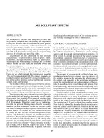
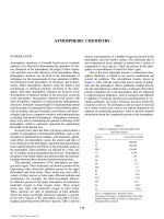
When the inverse-square law applies, then sound levels
decrease with distance at the rate: 20 lg r. Thus, if sound
level is known at one location, it may be estimated at another
location. Table 4 and Figure 3 show the distance adjustment
to be added to sound level at distance r
1
from the source to
obtain the sound level at distance r
2
.
MEASUREMENT AND INSTRUMENTATION
Sound level meters. The sound level meter is the basic tool
for making noise surveys. A typical sound level meter is a
hand-held battery-powered instrument consisting of a micro-
phone, amplifiers, weighting networks, a rootmean-square
rectifier, and a digital or analog sound level display. The A-
weighting network is most commonly used. This network
so that sound level is displayed in dBA. When measuring out-
of-doors, a windscreen is used to reduce measurement error
due to wind impinging on the microphone. Integrating sound
level meters automatically calculate equivalent sound level. If
a standard sound level meter is used, equivalent sound level
may be calculated from representative measurements, using
the procedure described later.
Frequency analysis. The cause of a noise problem may
sometimes be detected by analyzing noise in frequency
bands. An octave band is a frequency range for which the
upper frequency limit is (approximately) twice the lower
TABLE 4

Spherical wave attenuation
r2/r1 ADJ
0.5 6.0
0.6 4.4
0.7 3.1
0.8 1.9
0.9 0.9
1.0 0.0
1.1 Ϫ0.8
1.2 Ϫ1.6
1.3 Ϫ2.3
1.4 Ϫ2.9
1.5 Ϫ3.5
1.6 Ϫ4.1
1.7 Ϫ4.6
1.8 Ϫ5.1
1.9 Ϫ5.6
2.0 Ϫ6.0
2.1 Ϫ6.4
2.2 Ϫ6.8
2.3 Ϫ7.2
2.4 Ϫ7.6
2.5 Ϫ8.0
2.6 Ϫ8.3
2.7 Ϫ8.6
2.8 Ϫ8.9
2.9 Ϫ9.2
3.0 Ϫ9.5
Distance adjustment based
on the inverse-square law.

L(r2) ϭ L(r1) ϩ ADJ.
Distance ratio r2/r1
Add to sound level at r1
10
5
0
–5
–10
0.5
1.0
1.5 2.0 2.5 3.0
FIGURE 3 Distance adjustment based on the inverse-square law.
Number of equal contributions
Add to level due to one source
10
8
6
4
2
0
1
2
345678910
FIGURE 2 Combining n equal contributions.
C014_003_r03.indd 773C014_003_r03.indd 773 11/18/2005 10:46:09 AM11/18/2005 10:46:09 AM
© 2006 by Taylor & Francis Group, LLC
electronically adjusts the signal in accordance with Table 1,
774 NOISE
limit. An octave band is identified by its center frequency
defined as follows:

fff
cLu
ϭ
[]
12/
(8.1)
where f
c
ϭ the center frequency, f
L
ϭ the lower band limit,
and f
u
ϭ the upper band limit, all in Hz. The center frequen-
cies of the preferred octave bands in the audible range are
31.5, 63, 125, 250 and 500 Hz and 1, 2, 4, 8 and 16 kHz. The
center frequencies of the preferred one-third-octave bands are
Real-time analyzers and Fast-Fourier-Transform (FFT)
analyzers examine a signal in all of the selected frequency
bands simultaneously. The signal is then displayed as a bar-
graph, showing the sound level contribution of each selected
frequency band.
Sound intensity measurement. Vector sound intensity
is the net rate or flow of sound energy. Vector sound inten-
sity measurements are useful in determining noise source
power in the presence of background noise and for location
of noise sources. Sound intensity measurement systems uti-
lize a two-microphone probe to measure sound pressure at

two locations simultaneously.
The signals are processed to determine the particle veloc-
ity and its phase relationship to sound pressure.
Calibration. Acoustic calibrators produce a sound level
of known strength. Before a series of measurements, sound
measurement instrumentation should be adjusted to the cali-
brator level. Calibration should be checked at the end of each
measurement session. If a significant change has occurred,
the measured data should be discarded. Calibration data
should be recorded on a data sheet, along with instrumenta-
tion settings and all relevant information about the measure-
ment site and environmental conditions.
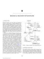
Background noise. When measuring the noise contribu-
tion of a given source, all other contributions to total noise
are identified as background noise. Let the sound level be
measured with the given source operating, and then let back-
ground noise alone be measured. The correction for back-
ground noise is given by


COR 10 lg 1 10
DIF 10
ϭϪ
Ϫ ⁄
⎡
⎣
⎤
⎦

(8.2)

where DIF ϭ Total noise level – background noise level,
and the noise level contribution of the source in question is
given by:



L
SOURCE
Total noise level COR.ϭϩ
Background noise corrections are tab
plotted in Figure 4. Whenever possible measurements should
be made under conditions where background noise is negli-
gible. When total noise level exceeds background noise by at
least 20 dB, then the correction is less than 1/20 dB. Such ideal
conditions are not always possible. Truck noise, for example,
must sometimes be measured on a highway with other moving
vehicles nearby. If the difference between total noise level and
background noise is less than 5 dB, then the contribution of
the source in question cannot be accurately determined.
HEARING DAMAGE RISK
The frequency range of human hearing extends from about
20 Hz to 20 kHz. Under ideal conditions, a sound pressure
level of 0 dB at 1 kHz can be detected. Human hearing is less
sensitive to low frequencies and very high frequencies.
Hearing threshold. A standard for human hearing has
been established on the basis of audiometric measurements
at a series of frequencies. An individual’s hearing threshold
represents the deviation from the standard or audiometric-
zero levels. A hearing threshold of 25 dB at 4 kHz, for example,

indicates that an individual has “lost” 25 dB in ability to hear
sounds at a frequency of 4 kHz (assuming the individual had
“normal” hearing at one time).
A temporary threshold shift (TTS) is a hearing thresh-
old change determined from audiometric evaluation before,
and immediately after exposure to loud noise. A measurable
permanent threshold shift (PTS) usually occurs as a result
of long-term noise exposure. The post-exposure audiometric
measurements to establish PTS are made after the subject has
been free of loud noise exposure for several hours. A com-
pound threshold shift (CTS) combines a PTS and TTS. There
is substantial evidence that repeated TTS’s translate into a
measurable PTS. Miller (1974) assembled data relating TTS,
CTS and PTS resulting from exposure to high noise levels.
Occupational Safety and Health Administration
(OSHA criteria. OSHA (1981, 1983) and the Noise Control
Act (1972) set standards for industrial noise exposure and
guidelines for hearing protection. OSHA criteria have resulted
in reduced noise levels in many industries and reduced the
incidence of hearing loss to workers. However, retrospective
studies have shown that some hearing loss will occur with
long-term exposure a OSHA-permitted sound levels.
The basic OSHA criterion level (CL) is a 90 dBA sound
exposure level for an 8 hour day. An exchange rate (ER)
of 5 dBA is specified, indicating that the permissible daily
Total - background level
Background noise correction.
0
–0.5
–1

–1.5
–2
–2.5
4.0 6.0 8.0
10.0
12.0
14.0 16.0 18.0
20.0
FIGURE 4 Background noise correction.
C014_003_r03.indd 774C014_003_r03.indd 774 11/18/2005 10:46:10 AM11/18/2005 10:46:10 AM
© 2006 by Taylor & Francis Group, LLC
those listed in the first column of Table 1 (Section 3).
ulated in Table 5 and
NOISE 775
exposure time is halved with each 5 dBA sound level increase.
The threshold level, the sound level below which no contribu-
tion is made to daily noise dose, is 80 dBA (threshold level is
not to be confused with hearing threshold). When noise expo-
sure exceeds the action level (85 dBA) a hearing conservation
program is to be implemented. A hearing conservation program
should include noise exposure monitoring audiometric testing,
employee training, hearing protection and record-keeping.
According to OSHA standards continuous noise expo-
sure (measurable on the slow-response scale of a sound level
meter) is not to exceed 1151 dBA. For sound levels L where
80 Յ L Յ 115 dBA allowable exposure time is given by


T
L

ϭϭ
Ϫ
Ϫ
82 82
5
⁄
⎡
⎣
⎤
⎦
⁄
⎡
⎣
⎤
⎦
⁄
(
)
⁄
( CL) ER
L90

(9.1)

where T ϭ allowable exposure time (hours/day). The result
is shown in Table 6.
Noise dose. When sound levels vary during the day, noise
dose is used as an exposure criterion. Noise dose is given by

DCT
i
N
%
ϭ
ϭ
100
ii
⁄
∑
1
where C ϭ actual exposure of an individual at a given sound
level (hr), T ϭ allowable exposure time at that level and N ϭ
the number of different exposure levels during one day. Noise
dose D
%
should not exceed 100%. As an alternative to moni-
toring and calculations, workers may wear dosimeters which
automatically measure and calculate daily dose.
An exchange rate of 3 dB is used in occupational noise
exposure criteria by some European countries. This exchange
rate is equivalent to basing noise exposure on L
eq
.
Environmental Protection Agency (EPA) identified
levels. Using a 4 kHz threshold shift criterion, protective
noise levels are substantially lower than the OSHA criteria.
EPA (1974, 1978) in its “Levels” document identified the
equivalent sound level of intermittent noise:

L
eq24
dBAϭ 70


as the “(at ear) exposure level that would produce no more
than 5 dB noise-induced hearing damage over a 40 year
period”. This value is based on a predicted hearing loss
smaller than 5 dB at 4 kHz for 96% of the people exposed
to 73 dBA noise for 8 hr/da ϫ 250 da/yr ϫ 40 yr. With the
following corrections, the 73 dBA level is adjusted to L
eq24
ϭ
70 dBA the protective noise level:
Ϫ1.6 dBA to account for 365 da/yr exposure,
Ϫ4.8 dBA to correct for 24 hr/day averaging,
ϩ5 dBA assuming intermittent exposure and
Ϫ1.6 dBA for a margin of safety.
NON-AUDITORY EFFECTS OF NOISE
The relationship between long-term exposure to industrial
noise and the probability of noise-induced hearing loss is
TABLE 5
Background noise correction
DIF COR DIF COR
0.2 Ϫ13.5 — —
0.4 Ϫ10.6 — —
0.6 Ϫ8.9 — —
0.8 Ϫ7.7 6.5 Ϫ1.1
1.0 Ϫ6.9 7.0 Ϫ1.0

1.2 Ϫ6.2 7.5 Ϫ0.9
1.4 Ϫ5.6 8.0 Ϫ0.7
1.6 Ϫ5.1 8.5 Ϫ0.7
1.8 Ϫ4.7 9.0 Ϫ0.6
2.0 Ϫ4.3 9.5 Ϫ0.5
2.2 Ϫ4.0 10.0 Ϫ0.5
2.4 Ϫ3.7 10.5 Ϫ0.4
2.6 Ϫ3.5 11.0 Ϫ0.4
2.8 Ϫ3.2 11.5 Ϫ0.3
3.0 Ϫ3.0 12.0 Ϫ0.3
3.2 Ϫ2.8 12.5 Ϫ0.3
3.4 Ϫ2.7 13.0 Ϫ0.2
3.6 Ϫ2.5 13.5 Ϫ0.2
3.8 Ϫ2.3 14.0 Ϫ0.2
4.0 Ϫ2.2 14.5 Ϫ0.2
4.2 Ϫ2.1 15.0 Ϫ
0.1
4.4 Ϫ2.0 15.5 Ϫ0.1
4.6 Ϫ1.8 16.0 Ϫ0.1
4.8 Ϫ1.7 16.5 Ϫ0.1
5.0 Ϫ1.7 17.0 Ϫ0.1
5.2 Ϫ1.6 17.5 Ϫ0.1
5.4 Ϫ1.5 18.0 Ϫ0.1
5.6 Ϫ1.4 18.5 Ϫ0.1
5.8 Ϫ1.3 19.0 Ϫ0.1
6.0 Ϫ1.3 19.5 Ϫ0.0
DIF ϭ total noise level–background
noise level. Sound level due to
source ϭ total noise level ϩ COR.
TABLE 6

Allowable exposure times
Time T
hr/da
Sound level L
dBA
32* 80
16 85
890
495
2 100
1 105
1/2 110
1/4 or less 115
*
The 32 hr exposure time is used
in evaluating noise dose when
sound levels vary.
C014_003_r03.indd 775C014_003_r03.indd 775 11/18/2005 10:46:10 AM11/18/2005 10:46:10 AM
© 2006 by Taylor & Francis Group, LLC
776 NOISE
well-documented. And, we can estimate the effect of intru-
sive noise on speech intelligibility and masking of warn-
ing signals. Equivalent sound levels and day-night sound
levels based on hearing protection, activity interference, and
Bureau identified noise as the top complaint about neighbor-
hoods, and the major reason for wanting to move. In a typi-
cal city, about 70% of citizen complaints relate to noise. The
most common complaints are aircraft noise, highway noise,
machinery and equipment, and amplified music.
Noise tolerance varies widely among individuals. It is

difficult to relate noise levels to psychological and non-
auditory physiological problems. But there is anecdotal evi-
dence that violent behavior can be triggered by noise. In a
New York case, one man cut off another man’s hand in a
dispute over noise. In another noise-related incident, a New
Jersey man operated his motorcycle engine inside his apart-
ment, leading a neighbor to shoot him.
Chronic noise exposure has been related to children’s
health and cognitive performance. In a study of British
schools, Stansfield and Haines (2000) compared reading
skills of students at four schools with 16-hour equivalent
sound levels less than 57 dBA and four schools with levels
greater than 66 dBA. After adjustment for socioeconomic
factors, lower average reading scores were found at the nois-
ier schools. The difference was equivalent to six months of
learning over four years.
A study by Zimmer et al. (2001) examined aircraft noise
exposure and student proficiency test results at three grade
levels. Communities with comparable socioeconomic status
were selected for the study. Noise-impacted communities
with a day-night sound level greater than 60 dBA and com-
munities with a level of less than 45 dBA were compared.
If proficiency test results are extrapolated to educational attain-
ment and salary level, one could predict a 3% salary level dis-
advantage for students from the impacted communities.
COMMUNITY NOISE
Contributors to community noise include aircraft, highway
vehicles, off-road vehicles, powered garden equipment,
construction activities, commercial and industrial activities,
public address systems and loud radios and television sets.

The major effects of community noise include sleep interfer-
ence, speech interference, and annoyance.
Highway noise. Noise levels due to highway vehicles
may be estimated from the Federal Highway Administration
(FHWA) model summarized by the sound level vs. speed
relationships in Table 7. These values make it possible to pre-
dict the impact of a proposed highway or highway improve-
ment on a community.
The contribution that a given class of vehicles makes to
hourly equivalent sound level is given by


LL DVSAAAA
A
S
eqH o o B D F G
lgϭϩ ϩϩϩϩ
ϩϪ
10
25
ր
[]

(10.1)

where D
o
ϭ 15 m, V ϭ volume (vehicles/hr), S ϭ speed
(km/hr). A
B, D, F, G

and
S
are adjustments for barriers, distance,
finite highway segments, grade and shielding due to buildings,
respectively. Each term is applied to a given class of vehicles
and traffic lane. For acoustically absorptive sites, the distance
adjustment is


ADD
Do
ϭ15lg ⁄
[]

(10.2)

where D ϭ distance from the traffic lane (m). Hourly equiva-
lent sound level at any location is predicted by combining the
contributions from all vehicle classes and traffic lanes. The
result is



L
i
eqH COMBINED
N
(
)
⁄

∑
ϭ
ϭ
10 10
10
1
lg .
LHieq

(10.3)

Design noise levels for highways. Design noise levels
specified by the Federal Highway Administration (1976) are
traffic on proposed highways are compared with the design
levels. These data aid in selecting a highway design and
routing alternative including the “no-build” alternative.
Aircraft noise. Noise contour maps are available for
most major airports. These enable one to make rough predic-
tions of the impact of aircraft noise on nearby communities.
Federal Aviation Administration publications (1985a and b)
outline aircraft noise certification procedures and aircraft
noise compatibility planning. Many of the existing airport
noise contour maps are based on the descriptor Noise expo-
sure forecast (NEF). An approximate conversion from NEF
to L
DN
is given by


L

DN
NEF 35ഠ ϩ

(10.4)

where L
DN
ϭ day-night sound level (Ϯ about 3 dBA).
Community noise criteria. There are thousands of dif-
ferent community noise ordinances, with a wide range of
permitted sound levels. Their effectiveness depends largely
on the degree of enforcement in a particular community. The
Environmental Protection Agency has identified the noise
TABLE 7
Energy mean emission levels for vehicles
Vehicle
class
Sound level
L
0
dBA
Speed S
km/hr
Autos
31.8 lg S Ϫ 2.4
у50
Autos 62 Ͻ50
Med. trucks
33.9 lg S ϩ 16.4
у50

Med. trucks 74 Ͻ50
Heavy trucks
24.6 lg S ϩ 38.5
у50
Heavy trucks 87 Ͻ50
Sound levels at 15 meters. Source: Barry and Reagan
(1978).
C014_003_r03.indd 776C014_003_r03.indd 776 11/18/2005 10:46:11 AM11/18/2005 10:46:11 AM
© 2006 by Taylor & Francis Group, LLC
annoyance are given in Table 9. The United States Census
summarized in Table 8. Noise predictions based on projected
NOISE 777
levels in Table 9 as protective of public health and welfare.
All are based on an average 24 hour day.
Control of community noise. Environmental noise
problems are particularly difficult to solve due to problems
of shared responsibility and jurisdiction. In many cases,
Federal laws preempt community regulations. Highway
noise and aircraft noise, often the most significant contribu-
tors to community noise levels, are largely exempt from local
control. In spite of the difficulties encountered, however, the
importance of protecting the quality of life makes environ-
mental noise control efforts worthwhile. Depending on the
circumstances, some of the following courses of action may
be considered.
a) Review the applicable noise ordinance. Compare
it with a model noise ordinance. Check to see if
specific limits are set in terms dBA. Determine
whether or not sound level meters are available and
whether or not the ordinance is actually enforced.

b) Meet with representatives of the local governing
body or environmental commission. Make them
aware of noise related problems in the community.
c) Initiate a campaign for public awareness with
regard to the environment including the noise
environment. Make use of the local papers.
d) Consider a ban or limitation on all-terrain- vehicles
(ATV’s). Determine whether muffler requirements
are actually enforced.
e) Encourage planning and zoning boards to require
an environmental impact statement (EIS), including
a noise report, before major projects are approved.
f) Support noise labeling for lawn mowers and other
power equipment.
g) Attend and participate in hearings involving plans
for airports, heliports, and highways. Consider
noise impact when evaluating the cost/benefit
ratio for proposed facilities.
h) Evaluate the feasibility of noise barriers on exist-
ing and proposed highways in sensitive areas.
i) Support legislation to reduce truck noise emission
limits.
j) Support legislation enabling airport curfews.
REFERENCES
Barry, T.M. and Reagan, J.A. FHW A highway traffic noise prediction
model FHWA-RD-77-108, 1978.
Environmental Protection Agency, Information on levels of environmental
noise requisite to protect public health and welfare with an adequate
margin of safety, EPA 550/9-74-004, 1974.
Environmental Protection Agency, Model community noise control ordinance,

EPA 550/9-76-003, 1975.
Environmental Protection Agency, Protective noise levels, EPA 559/979-100,
1978.
Federal Aviation Administration, Noise standards: aircraft type and air-
worthiness certification, FAR part 36, 1985(a).
Federation Aviation Administration, Airport noise compatibility planning,
FAR part 150, 1985(b).
Federal Highway Administration, Procedures for abatement of highway
traffic noise and construction noise, FHPM 7-7-3, 1976.
Federal Register, Code of federal regulations, 29, parts 1900 to 1910, 1985.
Miller, J.D., “Effects of noise on people,” J. Acoust Soc. Am. 56, no. 3,
pp. 729–764, 1974.
Noise control act of 1972, PL 92-574, HR 11021, Oct. 27, 1972.
Occupational Safety and Health Administration, “Occupational noise
exposure hearing conservation amendment” Federal Register, 46 (11),
4078–4181 and 46 (162), 42622–42639, 1981.
Occupational Safety and Health Administration, “Guidelines for noise enforce-
ment”, OSHA Instruction, CPL2-2.35,29 CFR1910.95(6) (1), 1983.
Peterson, A.P.G., Handbook of noise measurement, GenRad, Concord, MA,
9th ed., 1980.
Stansfield, S. and M. Haines, “Chronic aircraft noise exposure and chil-
dren’s cognitive performance and health: the Heathrow studies”, FICA
symposium, San Diego CA, 2000.
Wilson, C., Noise Control, Krieger, Malabar FL, 1994.
Zimmer, I.B., R. Dresnack, and C. Wilson, Modeling the impact of aircraft
noise on student proficiency”, NOISE-CON Portland ME, 2001 .
The following Internet resources may contain current information of interest:
www.faa.gov Federal Aviation Administration
www.icao.int International Civil Aviation Administration
www.fhwa.dot.gov. Federal Highway Administration

environment/noise
www.osha.gov Occ upational Safety and Health
Administration
TABLE 8
Design noise levels
Sound level
L
eqH
dBA
Measurement
location Land use category
57 Exterior Tracts of land in which
serenity and quiet are of
extraordinary
significance.
67 Exterior Residences, schools,
churches, libraries,
hospitals, etc.
72 Exterior Commercial and other
activities.
52 Interior Residences, schools,
churches, libraries,
hospitals, etc.
TABLE 9
Protective noise levels
Effect Level (dBA) Area
Hearing protection
L
eq24
р 70

All areas. See Section 9.
Outdoor activity
L
DN
р 55
Outdoors in residential
areas.
Interference and annoyance
L
eq24
р 55
Outdoor areas where
people spent limited
amounts of time.
Indoor activity
L
DN
р 45
Indoor residential areas.
Interference and annoyance
L
eq24
р 45
Other indoor areas with
human activities such as
schools, etc.
Source: EPA (1974, 1979).
C014_003_r03.indd 777C014_003_r03.indd 777 11/18/2005 10:46:11 AM11/18/2005 10:46:11 AM
© 2006 by Taylor & Francis Group, LLC
778 NOISE

www.cdc.gov/niosh Nat ional Institute for Occupational Safety and
Health
europe.osha.eu.int Eur opean Agency for Safety and Health
at Work
europa.eu.int. European Union
en/record/green
www.epa.gov Environmental Protection Agency
www.who.int/ World Health Organization
environmental_
information/noise
CHARLES E. WILSON
New Jersey Institute of Technology
C014_003_r03.indd 778C014_003_r03.indd 778 11/18/2005 10:46:11 AM11/18/2005 10:46:11 AM
© 2006 by Taylor & Francis Group, LLC