ENCYCLOPEDIA OF ENVIRONMENTAL SCIENCE AND ENGINEERING - PPARTICULATE EMISSIONSEMISSION STANDARDS doc

817
P
PARTICULATE EMISSIONS
EMISSION STANDARDS
Allowable levels of particulate emissions are specified in
several different ways, having somewhat different meth-
odologies of measurement and different philosophies of
important criteria for control. Permissible emission rates are
in a state of great legislative flux both as to the definition
of the suitable measurement and to the actual amount to be
allowed. This section summarizes the various types of quan-
titative standards that are used in regulating particulate emis-
sions. For a detailed survey of standards, the reader should
consult works by Stern,
1
Greenwood et al. ,
2
and the Public
Health Service.
3

A recent National Research Council report proposes
future studies on the nature of particulate emissions, their
effect on exposed populations and their control
4
. Friedrich
and Reis
5
have reported the results of a 10-year multinational
European study on characteristics, ambient concentrations
and sources of air pollutants.

The following paragraphs give an overview of standards
for ambient particulate pollution and source emission. The
precise and practical methodology of making accurate and/
or legally satisfactory measurements is beyond the scope of
this article. Books such as those by Katz,
6
Powals et al. ,
7

Brenchly et al. ,
8
and Hawksley et al.
9
should be consulted
for detailed sampling procedures. In the Federal Register
USEPA announced the implementation of the PM-10 regu-
lations (i.e., portion of total suspended particulate matter of
10 µ m or less particle diameter).
40,41

Ringlemann Number
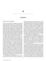
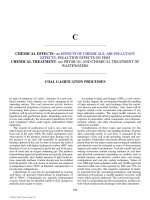
Perhaps the first attempt at quantifying particulate emis-
sions was developed late in the 19th century by Maximilian
Ringlemann. He developed the concept of characterizing a
visible smoke plume according to its opacity or optical den-
sity and originated the chart shown in Figure 1
as a conve-
nient scale for estimation of opacity. The chart consists of
four grids of black lines on a white background, having frac-
tional black areas of 20, 40, 60 and 80% which are assigned

Ringlemann Numbers of 1–4. (Ringlemann 0 would be all
white and Ringlemann 5 all black.) For rating a smoke plume,
the chart is held at eye level at a distance such that chart lines
merge into shades of grey. The shade of the smoke plume is
compared to the chart and rated accordingly. The history and
use of the Ringlemann chart is covered by Kudlich
8
and by
Weisburd.
9

In actual practice, opacity is seldom determined by use
of the chart, although the term Ringlemann Number persists.
Instead, observers are trained at a “smoke school.”
10
Test
plumes are generated and the actual percentage of light atten-
uation is measured spec-trophotometrically within the stack.
Observers calibrate their perception of the emerging plume
against the measured opacity. Trained observers can usu-
ally make readings correct to Ϯ 1/2 Ringlemann number.
11,13

Thus, with proper procedures, determination of a Ringlemann
Number is fairly objective and reproducible.
The Ringlemann concept was developed specifically for
black plumes, which attenuate skylight reaching the observ-
er’s eye and appear darker than the sky. White plumes, on
the other hand, reflect sunlight and appear brighter than the
background sky so that comparison to a Ringlemann chart is

meaningless. The smoke school approach is quite applicable,
however. Observations of a white plume are calibrated against
the measured light attenuation. Readings of white plumes are
somewhat more subject to variation due to relative locations
of observer, plume, and sun. It has been found that observa-
tions of equivalent opacity taken with the observer facing
the sun are about 1 Ringlemann number higher
13
than those
FIGURE 1 Ringlemann’s scale for grading the density of smoke.
C016_001_r03.indd 817C016_001_r03.indd 817 11/18/2005 1:15:33 PM11/18/2005 1:15:33 PM
© 2006 by Taylor & Francis Group, LLC
818 PARTICULATE EMISSIONS
taken in the prescribed method with the sun at the observer’s
back. Nevertheless, when properly made, observations of
Ringlemann numbers are reproducible among observers and
agree well with actual plume opacity.
Opacity regulations specify a maximum Ringlemann
number allowable on a long-term basis but often permit
this to be exceeded for short prescribed periods of time. For
instance, a typical requirement specifies that emissions shall
not exceed Ringlemann 1, except that for up to 3 min/hr emis-
sions up to Ringlemann 3 are permitted. This allowance is of
considerable importance to such operation as soot blowing
or rapping of electrostatic precipitator plates, which produce
puffs to smoke despite on overall very low emission level.
Federation regulations of the Environmental Protection
Agency
14
specify that opacity observations be made from a

point perpendicular to the plume, at a distance of between
two stack heights and one quarter of a mile, and with the sun
at the observer’s back. For official certification, an observer
under test must assign opacity readings in 5% increments
(1/4 Ringlemann number) to 25 plumes, with an error not
to exceed 15% on any single reading and an average error
(excluding algebraic sign of individual errors) not to exceed
7.5%. Annual testing is required for certification. In view of
previous studies,
11,13
this is a very high standard of perfor-
mance and probably represent the limits of visual quantifica-
tion of opacity.
Perhaps the greatest advantage of the Ringlemann Number
approach is that it requires no instrumentation and very little
time and manpower. Readings can usually be made by con-
trol authorities or other interested parties without entering the
premises of the subject source. Monitoring can be done very
frequently to insure continual, if not continuous, compliance
of the source. Finally, in terms of public awareness of par-
ticulate emissions, plume appearance is a logical candidate
for regulation. Air pollution is, to a great extent, an aesthetic
nuisance affecting the senses, and to the extend that plume
appearance can be regulated and improved, the visual impact
of pollution is reduced.
The Ringlemann Number concept has drawbacks reflecting
its simple, unsophisticated basis. Most serious is that, at pres-
ent, there is no really quantitative relationship between stack
appearance and the concentration of emissions. Additional
factors; such as particle size distribution, refractive index,

stack diameter, color of plume and sky, and the time of day,
all have a marked effect on appearance. On a constant weight
concentration basis, small particles and large smoke stacks will
produce a poor Ringlemann Number. Plumes that have a high
color contrast against the sky have a very strong visual impact
that does not correspond closely to the nature of the emissions.
For example, a white plume may be highly visible against a
deep blue sky, but the same emission can be practically invis-
ible against a cloudy background. As a result, it is often dif-
ficult to predict whether or not proposed control devices for a
yet unbuilt plant will produce satisfactory appearance. Certain
experience factors are presented in Table 1 for emissions, mea-
sured on a weight concentration basis, which the Industrial Gas
Cleaning Institute has estimated will give a Ringlemann 1 or
a clear stack.
A second objection is that Ringlemann number is a
purely aesthetic measurement which has no direct bearing
on physiological effects, ambient dirt, atmospheric corro-
sion, or any of the other very real and costly effects of par-
ticulate air pollution. There is some concern that regulations
of very low Ringlemann numbers will impose very costly
control measures upon sources without producing a com-
mensurate improvement in the quality of the environment.
Thus a high concentration of steam will produce a visually
prominent plume, but produce virtually no other undesirable
effects. Opacity restrictions are usually waived if opacity is
due entirely to steam but not if any other particles are pres-
ent, even if steam may be the major offender.
Instrumental Opacity
Many factors affecting the visual appearance of a smoke

plume are external variables, independent of the nature of the
emissions. In addition, visual reading cannot be taken at all
at night; and manpower costs for continuous daytime moni-
toring would be prohibitive. For these reasons, instrumental
measurements of plume opacity are sometimes desirable.
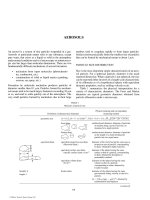
A typical stack mounted opacity meter is shown in
path traversing the smoke stack, and a phototube receiver
which responds to the incident light intensity and, hence,
to the light attenuation caused by the presence of smoke.
Various techniques including beam splitting, chopper stabi-
lization, and filter comparison are used to maintain stable
baselines and calibrations. At present, however, there is no
way to distinguish between dust particles within the gas
stream and those which have been deposited on surfaces in
the optical path. Optical surfaces must be clean for mean-
ingful measurements, and cleanliness is difficult to insure
for long periods of time in dusty atmosphere. The tendency,
therefore, is for such meters to read high, indicating more
smoke than is actually present. For this reason, and because
of reluctance to have a continuous record of emissions, there
has not been a very strong push by industries to supplant
Ringlemann observations with opacity meters.
Stack mounted opacity meters, of course, will not detect
detached plumes, which may contribute to a visual Ringlemann
observation. Detached plumes are due to particles formed by
condensation or chemical reaction after gas leaves the stack
and are thus beyond detection of such a meter.
At present, Texas is the only state with emissions control
regulations based on use of opacity meters,
15

as described
by McKee.
11
The Texas regulations is written so that smoke
of greater optical density (light attenuation per unit length
of light path) is permitted from low velocity stacks or small
diameter ones. Basically, a minimum transmittance of 70%
is allowed across the entire (circular) stack diameter if the
stack has an exit velocity of 40 ft/sec, and adjustment equa-
tions are provided for transmittance and/or optical path
length if non-standard velocity or path length is used.
Perhaps the greatest dissatisfaction with emission regula-
tions based either on visual observation number or on instru-
mental opacity is due to the fact that there is presently no
C016_001_r03.indd 818C016_001_r03.indd 818 11/18/2005 1:15:34 PM11/18/2005 1:15:34 PM
© 2006 by Taylor & Francis Group, LLC
Figure 2. It consists, basically, of a light source, an optical
PARTICULATE EMISSIONS 819
TABLE 1
Industrial process emissions expected to produce visually clear (or near clear) stack
Industrial classification Process Grains/ACF @Stack exit temp. (°F)
Utilities and industrial power plant fuel
fired boilers
Coal—pulverized 0.02 @ 260–320
Coal—cyclone 0.01 @ 260–320
Coal—stoker 0.05 @ 350–450
Oil 0.003 @ 300–400
Wood and bark 0.05 @ 400
Bagasse Fluid 0.04 @ 400
Fluid code 0.015 @ 300–350

Pulp and paper Kraft recovery boiler 0.02 @ 275–350
Soda recovery boiler 0.02 @ 275–350
Lime kiln 0.02 @ 400
Rock products—kiln Cement—dry 0.015 @ 450–600
Cement—wet 0.015 @ 450–600
Gypsum 0.02 @ 500
Alumina 0.02 @ 400
Lime 0.02 @ 500–600
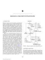
Bauxite 0.02 @ 400–450
Magnesium oxide 0.01 @ 550
Steel Basic oxygen furnace 0.01 @ 450
Open hearth 0.01–0.015 ≈450–600
Electric furnace 0.015 @ 400–600
Sintering 0.025 @ 300
Ore roasters 0.02 @ 400–500
Cupola 0.015 @ 0.02 ≈250–400
Pyrites roaster 0.02 @ 400–500
Taconite roaster 0.02 @ 300
Hot scarfing 0.025 @ 250
Mining and metallurgical Zinc roaster 0.01 @ 450
Zinc smelter 0.01 @ 400
Copper roaster 0.01 @ 500
Copper reverberatory furnace 0.015 @ 550
Copper converter 0.01 @ 500
Aluminum—Hall process 0.075 @ 300
Soderberg process 0.003 @ 200
Ilmenite dryer 0.02 @ 300
Titanium dioxide process 0.01 @ 300
Molybdenum roaster 0.01 @ 300
Ore beneficiation 0.02 @ 400

Miscellaneous Refinery cataly stregenerator 0.015 @ 475
Incinerators—Municipal 0.015 @ 500
Apartment 0.02 @ 350
Spray drying 0.01 @ 400
Precious meal—refining 0.01 @ 400
C016_001_r03.indd 819C016_001_r03.indd 819 11/18/2005 1:15:34 PM11/18/2005 1:15:34 PM
© 2006 by Taylor & Francis Group, LLC
820 PARTICULATE EMISSIONS
quantitative procedure for design of equipment to produce
complying plumes. Equipment vendors will usually guar-
antee collection efficiency and emission concentrations by
weight, but they will not give a guarantee to meet a specified
opacity. This is indeed a serious problem at a time when a
large precipitator installation can cost several million dollars
and take twenty months to fabricate and install. Overdesign
by a very conceivable factor of two can be very expensive in
unneeded equipment. Underdesign can mean years of delay
or operation under variance or with penalty payments.
Some progress has been made in applying classical theo-
ries of light scattering and transmission to the problem of
predicting opacity. This effort has been greatly hampered by
paucity of data giving simultaneous values of light attenua-
tion, particle size distribution, and particle concentration in
a stack. Perhaps the most comprehensive work to date has
been that of Ensor and Pilat.
16

Weight Limits on Particulates
Perhaps the least equivocal method of characterizing and
specifying limits on particulate emissions is according to

weight, either in terms of a rate (weight of emissions per unit
time) or in terms of concentration (weight per unit volume).
Measurement of emission weights must be done by iso-
kinetic sampling of the gas stream, as outlined in the follow-
ing section on measurement. Although the principles of such
measurement are simple, they are difficult and time consum-
ing when applied with accurate methodology to commer-
cial installations. For this reason, such measurements have
not previously been required in many jurisdictions and are
almost never used as a continual monitoring technique.
Limits on weight rate of emissions are usually dependent
on process size. Los Angeles, for instance, permits emissions
to be proportional to process weight, up to 40 lbs/hr particu-
lates for a plant processing 60,000 lbs/hr of material. Larger
plants are limited to 40 lbs/hr. For furnaces, the determining
factor is often heat input in BTU/hr rather than process weight.
In cases where a particular plant location may have several
independent units carrying out the same or similar processes,
regulations often require that the capacities be combined for
the purposes of calculating combined emissions.
Concentration limits are usually independent of process
size. For instance, the EPA specifies incinerator emission of
0.08 grains particulates per standard cubic foot of flue gas
(0.18 gm/NM
3
) Dilution of the flue gas with excess air is usu-
ally prohibited, or else correction must be made to standard
excess air or CO
2
.

Ground Level Concentrations of
Suspended Particulates
A limit on ground level concentration of particulates is an
attempt to regulate emissions in accordance with their impact
on population. A smoke stack acts as a dispersing device,
and such regulations give incentive to build taller stacks in
optimum locations.
In theory, ground level concentrations can be measured
directly. Usually, however, emissions are measured in the
stack, and plume dispersion equations are then used to cal-
culate concentration profiles. Plume dispersion depends on
stack height, plume buoyancy (i.e. density relative to ambi-
ent air), and wind velocity, and wind patterns. In addition,
plumes are never stationary but tend to meander; and cor-
rection factors are usually applied to adjust for the sampling
time at a fixed location. Dispersion calculations are usually
easier than direct ground level measurements; and in cases
where many different sources are present, calculation offers
the only practical way to assess the contributions of a spe-
cific source. A recent evaluation of plume dispersion models
is given by Carpenter et al.
15

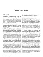
In some states, a plume dispersion model is incorporated
into a chart which gives an allowable weight rate of emissions
as a function of effective stack height and distance from prop-
erty lines. An example of this approach is shown in Figure 3.
FIGURE 3 Emission requirements for fine particles
based on plume dispersion model (New Jersey Air Pollution
Code).

FIGURE 2 Stack mounted opacity meter (Bailey Meter
Co.).
SPOTLAMP
LIGHT SOURCE
SPACED FLANGES
FOR AIR INLET
SMOKE OR DUST
PASSAGE
BOLOMETER
SPACED FLANGES
FOR AIR INLET
C016_001_r03.indd 820C016_001_r03.indd 820 11/18/2005 1:15:34 PM11/18/2005 1:15:34 PM
© 2006 by Taylor & Francis Group, LLC
PARTICULATE EMISSIONS 821
The particular regulation shown also accounts for differing
toxicity of certain particulates and allocates the emission
factors of Table 2 accordingly.
Very often permissible ground level concentrations are
set according to other sources in the area. Thus a plant would
be allowed greater emissions in a rural area than in a heavily
industrialized neighbourhood.
Dust fall
A variant on the ground level concentration limit is a dustfall
limit. This basically superimposes a particle settling velocity
on ground level concentration to obtain dustfall rates in weight
per unit area per unit time. This is a meaningful regulation
only for large particles and is not widely legislated at present.
Federal Clean Air Statutes and Regulations
The major federal statutes covering air pollution are PL 88– 206
(The Clean Air Act of 1963), PL 90–148 (The Air Quality Act

of 1967) PL 92–157, PL 93–115, PL 95–95 (The Clean Air
amendments of 1977), and PL 95–190, Administrative stan-
dards formulated by the Environmental Protection Agency
(EPA) are given in the Code of Federal Regulations Title 40,
parts 50, 51, 52, 53, 58, 60, 61, and 81.

The EPA has established National Ambient Air Quality
Standards (NAAQS). For suspended particulate matter the
primary standard (necessary to protect the public health with
an adequate margin of safety) is 75 µ g/M
3
annual geometric
mean with a level of 260 µ g/M
3
not to be exceeded more
than once per year. All states have been required to file state
implementation plants (SIP) for achieving NAAWS. It is
only through the SIP’s that existing pollution sources are
regulated.
The EPA requires no specific state regulations for
limits on existing sources, but suggestions are made for
“emission limitations obtainable with reasonable available
technology.” Some of the reasonable limits proposed for
particulates are:
1) Ringlemann 1 or less, except for brief periods
such as shoot blowing or start-up.
2) Reasonable precautions to control fugitive dust,
including use of water during grading or demo-
lition, sprinkling of dusty surfaces, use of hoods
and vents, covering of piles of dust, etc.

3) Incinerator emission less than 0.2 lbs/100 lbs
refuse charged.
4) Fuel burner emissions less than 0.3 lbs/million
BTU heat input.
5) For process industries, emission rates E in lbs/hr
and Process weight P in tons/hr according to the
relationships:
E = 3.59 P
0.62
for P р 30 tons/hr.
E = 17.31 P
0.16
for P у 30 tons/hr.
“Process weight” includes all materials introduced to the
process except liquid and gaseous fuels and combustion
air. Limits should be set on the basis of combined process
weights of all similar units at a plant.
In considering what emission limits should be estab-
lished, the states are encouraged to take into account local
condition, social and economic impact, and alternate control
strategies and adoption of the above measures is not manda-
tory. It is expected, however, that such measures will become
the norm in many areas.
For new or substantially modified pollution sources, the
EPA has established new source performance standards. The
standards for particulate emissions and opacity are given in
Table 3. Owners may submit plants of new sources to the
EPA for technical advice. They must provide ports, plat-
forms, access, and necessary utilities for performing required
tests, and the EPA must be allowed to conduct tests at rea-

sonable times. Required records and reports are available
to the public except where trade secrets would be divulged.
The states are in no way precluded from establishing more
stringent standards or additional procedures. The EPA test
method specified for particulates measures only materials
collectable on a dry filter at 250°F an does not include so
called condensables.
TABLE 2
Pollution Control Code)
Material Effect factor
Fine Solid Particles
All materials not specifically listed hereunder 1.0
Antimony 0.9
A-naphthylthiourea
0.5
Arsenic 0.9
Barium 0.9
Beryllium 0.003
Cadmium 0.2
Chromium 0.2
Cobalt 0.9
Copper 0.2
Hafnium 0.9
Lead 0.3
Lead arsenate 0.3
Lithium hydride 0.04
Phosphorus 0.2
Selenium 0.2
Silver 0.1
Tellurium 0.2

Thallium 0.2
Uranium (soluble) 0.1
Uranium (insoluble) 0.4
Vanadium 0.2
C016_001_r03.indd 821C016_001_r03.indd 821 11/18/2005 1:15:34 PM11/18/2005 1:15:34 PM
© 2006 by Taylor & Francis Group, LLC
Emission effect factors (for use with Fig. 3) (New Jersey Air
Chapter 1, Sub-chapter C, with regulations on particulates in
822 PARTICULATE EMISSIONS
In addition to new source performance standards, major
new stationary sources and major modifications are usually
subject to a “Prevention of Significant Deterioration” review.
If a particulate source of more than 25 tons/year is located
in an area which attains NAAQS or is unclassifiable with
respects to particulates, the owner must demonstrate that the
source will not violate NAAQS or PSD concentration incre-
ments. This requires modelling and preconstruction moni-
toring of ambient air quality. If the new or expanded source
is to be located in an area which does not meet NAAQS, then
emission from other sources must be reduced to offset the
new source. The regulation regarding emission offsets and
prevention of significant deterioration are relatively recent.
A summary of federal regulations as of 1981 has recently
been published as a quick guide to this rapidly changing
field.
18

In recent years, regulation of particulate emissions from
mobile sources has been initiated. The burden is essentially
on manufacturers of diesel engines. Because the emission

requirements and test procedures are quite complex and
because the target is highly specific, a comprehensive discus-
sion is beyond the scope of this article. Some representative
standards are: Diesel engines for urban buses, 0.019 grams/
megajoule, and other diesel engines for road use, 0.037 grams/
megajoule:
19
Non-road diesel engines, 1 gram/kilowatt-hour
for sizes less than 8 kilowatts in tier 1 down to 0.2 grams/
kilowatt-hour for units larger than 560 kilowatts in tier 2.
20

Locomotives, 0.36 grams/bhp-hr for switching service in tier
1 down to 0.1 grams/bhp-hr for line service in tier 3.
21
Marine
diesel engines, 0.2 grams/KwH to 0.5 grams/KwH, depending
on displacement and tier.
22
Note that the emission units above
are as specified in the printed regulation.
Particulate emission standards are also being promulgated
by agencies other than the Environmental Protection Agency.
In general, these are workplace standards. An example
would be the standard for mobile diesel-powered transporta-
tion equipment promulgated by the Mine Safety and Health
Administration. This specifies that the exhaust “shall not con-
tain black smoke.”
23

MEASUREMENT OF PARTICULATE EMISSIONS
As a first step in any program for control of particulate emis-
sions, a determination must be made of the quantity and
nature of particles being emitted by the subject source. The
quantity of emissions determines the collection efficiency
and size of required cleanup equipment. The particle size and
chemical properties of the emitted dust strongly influence
the type of equipment to be used. Sampling for this purpose
has been mainly a matter of industrial concern. A last step
in most control programs consists of measuring pollutants
in the cleaned gas stream to ensure that cleanup equipment
being used actually permits the pertinent emission targets to
be met. With increasing public concern and legislation on air
pollution, sampling for this purpose is increasingly required
by statute to determine compliance with the pertinent emis-
sion regulations. To this end the local pollution control
authority may issue a comprehensive sampling manual
which sets forth in considerable detail the procedures to be
used in obtaining raw data and the computations involved in
calculating the pertinent emission levels.
Complete and comprehensive source testing procedures
are beyond the scope of this paper. References 24–28 give
detailed instruction for performance of such tests.
Sampling of gas streams, especially for particulates, is
simple only in concept. Actual measurement require special-
ized equipment, trained personnel, careful experimental and
computational techniques, and a considerable expenditure
of time and manpower. Matters of technique and equipment
are covered in source testing manuals as mentioned above
and are briefly summarized later in this paper. Two addi-

tional complicating factors are usually present. First is the
frequent inaccessibility of sampling points. These points are
often located in duct work 50–100 ft above ground level.
Scaffolding must often be installed around the points, and
several hundred pounds of equipment must be lifted to that
level. Probe clearances are often critical, for in order to make
a sample traverse on 12 ft dia. stack, a 14 ft probe is needed,
and clearance must be available for insertion into the sam-
pling port as well as a means for suspending the probe from
above. At least one professional stack sampler is an ama-
teur mountain climber and puts his hobby to good use on
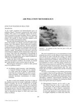
the job. A second complicating factor is the adverse physical
conditions frequently encountered. A somewhat extreme but
illustrative example is a refinery stream recently sampled. Gas
temperature was 1200°F requiring special probes and gas-
kets and protective clothing for the workers. The gas stream
contained 10% carbon monoxide creating potential hazards
of poisoning and explosion especially since duct pressure
was slightly above that of the atmosphere. Temperature in
the work area was in excess of 120°F contributing further to
the difficulty of the job.
In preparation for a sampling program, work platforms
or scaffolding and valved sample ports must be installed.
All special fittings for adapting the sampling probes to the
ports should be anticipated and fabricated. Arrangements
must be made with plant operating personnel to maintain
steady operating conditions during the test. The test must
be carefully planned as to number and exact location of tra-
verse sample points, and probes should be premarked for
these locations. Flow nomographs for sampling nozzles

should be made; and all filters, impingers, and other ele-
ment of sampling trains should be tared. With that advance
preparation a 3 man sampling team would require 1–2 days
to position their equipment and make gas flow measure-
ments and 2 sample transverses at right angles in a large
duct or stack.
Measurement of Gas Flow Rates
A preliminary step in determination of emission rates from
a stack is measurement of the gas flow rate. Detailed pro-
cedures in wide use including the necessary attention to
technique have been published by the ASME,
20
ASTM,
19

the Environmental Protection Agency, referred to as EPA,
21

C016_001_r03.indd 822C016_001_r03.indd 822 11/18/2005 1:15:34 PM11/18/2005 1:15:34 PM
© 2006 by Taylor & Francis Group, LLC
PARTICULATE EMISSIONS 823
TABLE 3
Federal Limits of Particulate Emissions from New Stationary Sources
(Through 2004 Codified in CFR, Title 40. Chapter 1/Part 60)
Subpart Source Particulate Emissions Opacity (%)
D Fossil fired steam generators 13 ng/j 20*
(27% for 6 min/hr)
Da Electric utility steam generators 43 ng/j 20*
(27% for 6 min/hr)
Db Industrial/commercial/institutional 22 to 86 ng/j 20*

steam generators depending on fuel, size, construction date (27% for 6 min/hr)
Dc Small industrial/commercial steam generators 22 to 43 ng/j 20*
depending on fuel, size (27% for 6 min/hr)
E Incinerators 0.18 g/dscm —
F Portland cement
kiln 0.15 kg/ton 20*
clinker cooler 0.05 kg/ton 10*
other facilities — 10
G Nitric acid — 10
H Sulfuric Acid 0.075 kg/ton 10
I Hot mix asphalt 90 mg/dscm 20
J Refinery—fluid catalytic cracker regenerator 1 kg/1000 kg coke burned 30*
(6 min/hr exception)
L Secondary lead smelters cupola or
reverberatory furnace 50 mg/dscm 20
pot furnace — 10
M Secondary brass and bronze production 50 mg/dscm 20
N Basic oxygen steel, primary emission 50 mg/dscm 10
with closed hooding 68 mg/dscm (20% once per production cycle)
Na Basic oxygen steel, secondary emissions
from shop roof — 10
(20% once per production cycle)
from control device 23 mg/dscm 5
O Sewage plant sludge incinerator 0.65 g/kg dry sludge 20
P Primary copper smelters, dryer 50 mg/dscm 20*
sulfuric acid plant — 20
Q Primary zinc smelters, sintering 50 mg/dscm 20*
sulfuric acid plant — 20
R Primary lead smelters, sintering or furnaces 50 mg/dscm 20*
sulfuric acid plant — 20

S Primary aluminum reduction
pot room — 10
Anode bake plant — 20
Y Coal preparation
thermal dryer 0.07 g/dscm 20
pneumatic coal cleaning 0.04 g/dscm 10
conveying, storage, loading — 20
(continued)
C016_001_r03.indd 823C016_001_r03.indd 823 11/18/2005 1:15:34 PM11/18/2005 1:15:34 PM
© 2006 by Taylor & Francis Group, LLC
824 PARTICULATE EMISSIONS
TABLE 3 (continued)
Subpart Source Particulate Emissions Opacity (%)
Z Ferroalloy production
control device; silicon, ferrosilicon, 0.45 kg/MW-hr 15*
calcium silicon or silicomanganese zirconium alloys
control device; production of other alloys 0.23 kg/MW-hr 15*
uncontrolled emissions from arc furnace — Not visible
uncontrolled emissions from tapping station — Not visible for more than 40% of
tap period
dust handling equipment — 10
AA Electric arc steel plants
control device 12 mg/dscm 3*
shop exit due to arc furnace operation — 6
except during charging — 20
except during tapping — 40
dust handling equipment — 10
BB Kraft pulp mills
recovery furnace
smelt dissolving tank

lime kiln, gas fired
oil fired
10 g/dscm
0.1 g/kg black liquor solids
0.15 g/dscm
0.30 g/dscm
35
—
—
—
CC Glass manufacture, standard process
container glass
pressed & blown glass, borosilisate
pressed & blown glass, soda lime & lead
pressed & blown glass, other compositions
wool fiberglass
flat glass
Gas fuel
l0.1 g/kg glass
0.5 g/kg
0.1 g/kg
0.25 g/kg
0.25 g/kg
0.225 g/kg
Oil fuel
l0.13 g/kg glass
0.65 g/kg
0.13 g/kg
0.325 g/kg
0.325 g/kg

0.225 g/kg
—
—
—
—
—
—
Glass manufacture, modified process
container, flat, pressed, blown glass, soda lime
container, flat, pressed, blown glass, borosilicate
textile and wood fiberglass
0.5 g/kg
1.0 g/kg
0.5 g/kg
*
*
*
DD Grain elevators
column dryer, plate perforation >2.4 mm
rack dryer, exhaust screen filter cans thru 50 mesh
other facilities
fugitive, truck unloading, railcar loading/unloading
fugitive, grain handling
fugitive, truck loading
fugitive, barge or ship loading
—
—
0.023 g/dscm
—
—

—
—
0
0
0
5
0
10
20
GG Lime rotary kiln 0.30 g/kg stone feed 15*
LL Metallic mineral processing
stack emissions
fugitive emissions
0.05 g/dscm
—
7
10
NN Phosphate rock
dyer
calciner, unbeneficiated rock
calciner, beneficiated rock
rock grinder
0.03 g/kg rock
0.12 g/kg rock
0.055 g/kg rock
0.0006 g/kg rock
10*
10*
10*
0*

PP Ammonium sulfate manufacture, dryer 0.15 g/kg product 15
(continued)
C016_001_r03.indd 824C016_001_r03.indd 824 11/18/2005 1:15:34 PM11/18/2005 1:15:34 PM
© 2006 by Taylor & Francis Group, LLC
PARTICULATE EMISSIONS 825
TABLE 3 (continued)
Subpart Source Particulate Emissions Opacity (%)
UU Asphalt roofing
shingle of mineral-surfaced roll
saturated felt or smooth surfaced roll
Asphalt blowing still
with catalyst addition
with catalyst addition, #6 oil afterburner
no catalyst
no catalyst, #6 oil afterburner
Asphalt storage tank
Asphalt roofing mineral handling and storage
0.04 g/kg
0.4 g/kg
0.67 g/kg
0.71 g/kg
0.60 g/kg
0.64 g/kg
20
20
—
—
—
—
0

1
AAA Residential wood heaters
with catalytic combustor
no catalytic combustor
4.1 g/hr
7.5 g/hr
—
—
OOO Nonmetallic mineral processing
stack or transfer point on belt conveyors
fugitive emissions
crusher fugitive emissions
0.05 g/dscm
—
—
7
10
15
PPP Wool fiberglass insulation 5.5 g/kg
UUU Calciners & dryers in mineral industries 0.092 g/dscm 10*
*Continous monitoring by capacity meters required
The above standards apply to current construction. Existing unmodified units may have lower standards.
Many applications require continuous monitoring of operating variables for process and control equipment.
the Lost Angeles Air Pollution Control district, referred
to as APCD,
21
and the Western Precipitation Division,
referred to as WP.
21
This article will only treat the general

procedures and not significant differences between popu-
lar techniques.
Velocity Traverse Points Because of flow non-uniformity,
which almost invariably occurs in large stacks, the stack
cross section in the sampling plane must be divided into a
number of smaller areas and gas velocity determined sepa-
rately in each area. Circular ducts are divided by concentric
circles, and 2 velocity traverses are made at right angles.
Figure 4 shows a typical example. Location of the sample
points can be determined from the formula

RD
n
N
n
ϭ
Ϫ21
2



where
R
n
= distance from center of duct to the “ n th” point
from the center
D = duct diameter
n = sample point number, counting from center
N = total number of measurement points in the duct. The
number of sample points along one diameter is N /2.

For rectangular ducts the cross section is divided into
N equal rectangular areas such that the ratio of length to
width of the areas is between one and two. Sample points are
at the center of each area.
The number of traverse points required is usually speci-
fied in the applicable test code as a function of duct area or
diameter. Representative requirements are shown in Table 4.
S-6
S-5
S-4
E-4E-5E-6 E-3 E-2 E-1
EAST
S-3
S-2
S-1
SOUTH
R
3
R
2
R
1
FIGURE 4 Velocity and sampling traverse positions
in circular ducts.
C016_001_r03.indd 825C016_001_r03.indd 825 11/18/2005 1:15:35 PM11/18/2005 1:15:35 PM
© 2006 by Taylor & Francis Group, LLC
826 PARTICULATE EMISSIONS
Very often more points are required if the flow is highly non-
uniform or if the sampling point is near an elbow or other
flow disturbance. Figure 5 shows the EPA adjustment for

flow nonuniformity.
Velocity Measurement Velocity measurements in dusty
gases are made with a type S (special or staubscheibe) pitot
tube, shown in Figure 6, and a draft gage manometer. Gas
velocity is given by

VCgh
LL
ϭ 2 rr/
g

where
V = gas velocity
C = pitot tube calibration coefficient. This would be
1.0 for an ideal pitot tube, but type S tubes deviate con-
siderably.
g = acceleration of gravity
h
L
= liquid height differential in manometer
␳
L
= density of manometer liquid
␳
g
= gas density.
It is necessary to measure the temperature and the pres-
sure of the gas stream and estimate or measure its molecular
weight in order to calculate density.
Gas Analysis For precise work gas composition is needed

for three reasons (1) so that molecular weight and gas density
may be known for duct velocity calculations, (2) so that duct
flow rates at duct condition can be converted to standard-
ized conditions used for emission specifications. Standard
conditions are usually 70°F, 29.91 in. mercury barometric
pressure, moisture free basis with gas volume adjusted to
TABLE 4
Required traverse points
Code Duct sizes Number of points
EPA
8
2 ft dia. 12 minimum
More according to Figure 2 if near flow disturbance
WP
17
<2 ft
2
>2–25 ft
2
25 ft
2
4
12
20 or more
APCD
14
and
ASTM
15
1–2 ft

2
(rectangular)
2–12 ft
2
>12 ft
2
1–2 ft dia.
2–4 ft
4–6 ft
>6 ft
4
6–24
24
12
16
20
24 or more
These numbers should be doubled where only 4–6 duct
diameters of straight duct are upstream.
ASME
16
<25 ft
2
>25 ft
2
8–12
12–20
Double or triple these numbers for high nonuniform flow.
MINIMUM NUMBER OF TRAVERSE POINTS
NUMBER OF DUCT DIAMETERS DOWNSTREAM*

(DISTANCE B)
DISTURBANCE
SAMPLING
DISTURBANCE
*FROM POINT OF ANY TYPE OF
DISTURBANCE (BEND, EXPANSION, CONTRACTION, ETC.)
NUMBER OF DUCT DIAMETERS UPSTREAM*
(DISTANCE A)
SITE
A
B
23 4 5 6 7 8 9 10
0
10
20
30
40
50
0.5 1.0 1.5 2.0 2.5
FIGURE 5 Sampling points required in vicinity of flow distur-
bance (EPA).
TUBLING ADAPTER
PIPE COUPLING
STAINLESS STEEL TUBLING
FIGURE 6 Type S Pitot tube for use in dusty gas
stream.
12% CO
2
. Some codes differ from this, however. (3) For iso-
kinetic sampling moisture content at stack conditions must

be known in order to adjust for the fact that probe gas flow is
measured in a dry gas meter at ambient conditions.
C016_001_r03.indd 826C016_001_r03.indd 826 11/18/2005 1:15:35 PM11/18/2005 1:15:35 PM
© 2006 by Taylor & Francis Group, LLC
PARTICULATE EMISSIONS 827
Gas analysis for CO
2
, CO, and O
2
is almost always done
by Orsat analysis. Moisture may be determined gravimetri-
cally by condensation from a measured volume of gas as
required by EPA.
Overall Flow Rate Total flow rate is calculated from duct
area and average gas velocity as determined by the pitot tube
measurements. Pitot tube traverse points are at the center of
equal areas so no weighting is necessary to determine aver-
age velocity. This gives flow at duct conditions which is usu-
ally converted to standard conditions.
Measurement of Particulate Concentrations in Stacks
Standard methods for measuring particulation concentrations
in stacks depend on the principle of isokinetic sampling. Since
particles do not follow gas streamlines exactly but tend to
travel in straight lines, precautions must be taken that the gas
being sampled experiences no change in velocity or direction
in the vicinity of the sampling point. This is done by using a
thin walled tubular probe carefully aligned with the gas flow
and by withdrawing gas so that velocity just within the tip of
the probe equals that in the main gas stream. Several recent
studies

29 – 31
have measured effects of probe size, alignment,
and velocity on accuracy of sampling. The sampled gas is
drawn through a train of filters, impingers, and a gas meter
by means of a pump or ejector. Typical probes are shown
in Figure 7, and several types are commercially available.
With these probes the necessary gas sampling velocity must
be previously determined by pitot tube measurement, and
the gas flow rate at the flow meter is adjusted (taking into
account gas volume changes due to cooling and condensation
between stack and meter) to equal that velocity. An alternate
method is to use a null nozzle, which contains static pressure
taps to the outside and inside surfaces of the sample probe as
shown in Figure 8. Flow through the probe is adjusted so that
the static pressures are equal at which point the velocities
inside and outside the probe should be the same. The null
nozzle greatly simplifies sampling, but null nozzles require
careful periodic calibration and are not generally used for
high precision work.
The sampling train of filters and impingers, which col-
lects the particles, is usually carefully specified in the test
method or governmental regulation in force. Differences
between sampling trains to some extent reflect different
technical solutions to the sampling problem but they also
reflect differences in the philosophy of what exactly should
be measured.
Perhaps the most widespread train will be that specified by
the EPA
14
for testing new emission sources, shown in Figure 9.

The original intent was to collect and measure not only par-
ticles which actually exist in the stack at stack conditions, but
also solids or droplets that can be condensed out of the stack
gas as it is cooled to ambient conditions. The filter is heated
to avoid condensation and plugging. The first two impingers
contain water to collect most of the condensables. The third
impinger is empty and serves as an additional droplet tray
while the fourth impinger is filled with silica gel to collect
residual water vapor. Although the impingers in the train col-
lect condensibles, present regulations are written only in terms
of the solid particulates which are collected in the filter.
Slatic tap
Slatic tap
6 - No.60 holes
17
12
2
3
4
3
6
3
4
5
8
1
2
5
8
1

8
1
1
1
5°
3
1
°
12
FIGURE 8 Null type nozzle for isokinetic sampling.
HEATED AREA
FILTER HOLDER
THERMOMETER
CHECK
VALVE
VACUUM
LINE
ICE BATH
VACUUM
GAUGE
MAIN VALVE
AIR-TIGHT
PUMP
DRY TEST METER
THERMOMETERS
STACK
WALL
PROBE
REVERSE-TYPE
PITOT TUBE

PITOT MANOMETER
ORIFICE
BY-PASS VALVE
IMPINGERS
IMPINGER TRAIN OPTIONAL. MAY BE REPLACED
BY AN EQUIVALENT CONDENSER
FIGURE 9 Environmental Protection Agency particulate sam-
pling train.
Smooth Bend
d
Angle
30° or less
Pipe thread connection
to thimble holder
d
R
R
R
.
2d
Ն
Knife-edge circular opening
with straight internal wall
A. Elbow Nozzle
Goose-neck Nozzle
B.
FIGURE 7 Nozzles for particulate sampling.
C016_001_r03.indd 827C016_001_r03.indd 827 11/18/2005 1:15:35 PM11/18/2005 1:15:35 PM
© 2006 by Taylor & Francis Group, LLC
828 PARTICULATE EMISSIONS

The ASME power test code,
27
in contrast, is designed to
measure performance of devices such as precipitators and
cyclones, and thus is concerned only with substances which
are particulate at conditions prevailing in the equipment. This
test usually used a filter assembly with the filter very close to
the sampling probe so that the filter may be inserted into the
stack avoiding condensation. No impingers are used.
To some extent filter characteristics are determined by
process conditions. Alundum thimbles and glass wool packed
tubes are used for high temperatures. If liquid droplets are
present at the filter inlet, glass-wool tubes are the only useful
collection devices, because conventional filters will readily
become plugged by droplets. Glass-wool collection greatly
complicates quantitative recovery of particles for chemical
or size analysis.
In sampling a large duct having several traverse points
for flow and particle measurement, particles for all points
on a traverse are usually collected in a single filter impinger
train, thus giving an average dust concentration. Each sample
point is sampled for an equal time but at its own isokinetic
velocity. The probe is then immediately moved to the next
point and the flow rate adjusted accordingly. Sample flow
rate is adjusted by rotameter or orifice readings, but total gas
flow during the entire test is taken from a dry meter.
Minimum sampling time or volume is often set by regu-
lation. Examples are:
Bay area
24

—Sample gas volume = 20 L
0.8
, where volume
is in standard cubic ft, and L is duct equivalent dia. in ft.
A maximum sampling rate of 3 SCFM is specified and a
minimum time of 30 min.
ASME
27
—Minimum of 2hr with at least 10 min at each
traverse point through two complete circuits.
APCD
25
—5–10 min/point for a total run of at least 1 hr.
Industrial gas cleaning institute —At least 2 hr or 150 ft
3

sample gas or until sample weight is greater than 30% of filter
weight.
Emissions are calculated from test volumes of weight of
particulates collected and volume of sample gas through the
gas meter. Care must be taken to include particles deposited on
tubing walls as well as those trapped by the filter. If conden-
sibles are to be included, the liquid from the impinger train is
evaporated to dryness, and the residue is weighed and included
with the particulates. Corrections to the gas volume depend on
sample train operation and on standard conditions for report-
ing emissions, and these are spelled out in detail in the specific
test codes to be used. Results are usually expressed both as
grains per cubic foot (using standard conditions defined in the
code) and as lbs/hr from the whole stack.

Measurement and Representation of Particle Size
A determination of the emitted particle size and size dis-
tribution is a desirable element in most control programs.
Collection efficiency of any given piece of equipment is a
function of particle size, being low for small particles and
high for large ones, and capital and operating costs of equip-
ment required increased steadily as the dust particle size
decreases.
Perhaps the simplest method of particle size measure-
ment, conceptually at least, is by microscope count. The
minimum size that can be counted optically is about 0.5 µ
which is near the wavelength of visible light. Electron micro-
scopes may be used for sizing of smaller particles. Counting
is a laborious procedure, and sample counts are often small
enough to cause statistical errors at the very small and very
large ends of the distribution. This method requires the small-
est sample size and is capable of giving satisfactory results.
Care must be taken in converting from the number distribu-
tion obtained by this method to mass distribution.
A second simple method is sieve analysis. This is com-
monly used for dry freely flowing materials in the size range
above 44 µ, a screen size designated at 325 mesh. Using spe-
cial shaking equipment and very delicate micromesh sieves
particles down to 10 µ can be measured. Error can be caused
by “blinding” of the sieve mesh and sticky or fine particles,
incomplete sieving, and particle fragmentation during siev-
ing. A sample size of at least 5–10 g is usually required.
Another class of measurement techniques is based on the
terminal falling velocity of particles in a gas (air). The quan-
tity measured is proportional to rd

2
, where r is particle density
and d is diameter. Hence a separate determination of density
is needed. One such device is the Sharples Micromerograph
(Sharples-Stokes Division, Penwalt Corporation, Warminster,
Pennsylvania). The device records the time for particles to fall
through a 2 m high column of air onto the pan of a continu-
ously recording balance. Templates are available to convert
fall time to rd
2
. The Micromerograph is mechanically and
electrically complex but easy to use. An objection is that a
significant fraction of the injected particles stick to the column
walls and do not reach the balance pan. This effect can some-
times be selective, and it thus gives a biased size distribution.
A second sedimentation device is the Roller elutria-
and air is passed upwards through it for a specified time.
A separation is effected with small particles being carried
overhead and large ones remaining in the tube. Often a series
of tubes of decreasing diameter are connected in a cascade
with each successive tube having a lower air velocity and
retaining finer particles. The Roller method was used quite
widely in the petroleum industry for many years. However, it
is slow, requires a large sample, does not give clean particle
size cuts, and is sensitive to tube orientation. It is therefore
being supplanted by newer methods.
A third sedimentation is centrifugal sedimentation. This
is the standard test method of the Industrial Gas Cleaning
Institute, and use of such devices of the Bahco type has been
standardized by the ASME.

32
The Bahco analyzer consists
of a rapidly spinning rotor and a superimposed radial gas
flow from circumference to center. Larger particles are cen-
trifuged to the outside diameter of the rotor, while small ones
are carried to the center with a cut point determined by gas
velocity and rotor speed.
Still another method is the Coulter Counter. In this
technique the test powder is dispersed in an electrolyte,
which is then pumped through a small orifice. Current flow
between electrodes on each side of the orifice is continuously
C016_001_r03.indd 828C016_001_r03.indd 828 11/18/2005 1:15:35 PM11/18/2005 1:15:35 PM
© 2006 by Taylor & Francis Group, LLC
tor tube, Figure 10. A powder sample is placed in the tube
PARTICULATE EMISSIONS 829
monitored. Passage of a particle through the orifice momen-
tarily reduces current to an extent determined by particle
size. The device electronically counts the number of par-
ticles in each of several size ranges, and a size distribution
can then be calculated. The method is capable of giving very
good results, and newer model counters are very fast.
A novel liquid phase sedimentation analyzer is the
Sedigraph (Micrometrics Instrument Corporation, Norcross,
Georgia). The particle sample dispersed in liquid is put into a
sample cell and allowed to settle. Mass concentration is con-
tinuously monitored be attenuation of an X-ray beam, and
this is mathematically related to particle size, X-ray location
and time. The instrument automatically plots particle diam-
eter as cumulative weight percent. The device can cover the
size range from 0.1–10 µ in a single operation, a much wider

range than can be conveniently analyzed by most analyzers.
Laser optics techniques relying on light scattering,
Fraunhofer diffraction, or light extinction are becoming
the method of choice in many applications. The Leeds and
Northrop “Microtrac” and Malvern Instruments Co. laser par-
ticle and droplet sizer are representative of such techniques.
These Instruments can measure particles in a flowing gas
stream, and thus can theoretically be used on line. More often a
collected particulate sample is dispersed in liquid for analysis.
Impingement devices such as the Anderson Impactor, or
in the impactors developed by May or Batelle, may be used
to measure particle sizes in situ in a combined sampling and
sizing operation. As is shown in Figure 11 such a device con-
sists of a series of orifices arranged to give gas jets of increas-
ing velocity and decreasing diameter, which jets impinge
on collection plates, Successive stages collect smaller and
smaller particles, and the size distribution of aspirated par-
ticles can be obtained from the weight collected on each stage
and the size “cut point” calibration of the stage. Several stud-
ies of calibrations have been published,
33 - 37
and discrepancies
have been pointed out.
38
Impactors must be operated at con-
stant known gas flow rate and for this reason are not capable
of giving true isokinetic sampling under conditions of fluc-
tuating duct velocity. This is one of the few types of devices
which may be applied to liquid droplets, which coalesce once
collected. It is capable of size determination well below 1 µ

(finer than most devices). Because it eliminates recovery
of particles from a filter and subsequent handling, it can be
useful in measuring distributions at low concentrations.
Most particles emitted to the atmosphere are approxi-
mately spherical so that the exact meaning of “diameter”
is not usually important in the context. For highly irregular
particles a great many different diameters many be defined,
each with particular applications. For purposes of particulate
control equipment, persistence of airborne dusts, and physi-
ological retention in the respiratory tract, the most meaning-
ful diameter is usually the “aerodynamic” diameter, that of
the sphere having the same free fall velocity as the particle
of interest. This is the diameter measured by sedimentation,
eleutriation, and inertial impaction techniques.
A large number of methods are available for expressing
particle size distributions, each having properties of fitting
certain characteristic distribution shapes or of simplifying
1
1
2
COLLECTION
CUP
SPRING
JET SPINDLE
GASKET
FIGURE 11 Stage of typical cascade impactor
(Monsanto).
FIGURE 10 Air classifier for subsieve particle size
analysis.
C016_001_r03.indd 829C016_001_r03.indd 829 11/18/2005 1:15:36 PM11/18/2005 1:15:36 PM

© 2006 by Taylor & Francis Group, LLC
830 PARTICULATE EMISSIONS
certain mathematical manipulations. A comprehensive sum-
mary of various distribution functions is given by Orr.
39
The
most useful function in emission applications seems to be the
long-normal distribution. Commercial graph paper is avail-
able having one logarithmic scale and one cumulative normal
probability scale. If particle size is plotted vs. cumulative
percentage of sample at or below that size, the log-normal
distribution gives a straight line. A large percentage of emis-
sions and ambient particulate distributions have log-normal
distributions, and plotting on log-probability paper usually
facilitates interpolation and extrapolation even when the line
is not quite straight. For a true log-normal distribution very
simple relationships permits easy conversion between distri-
butions based on number, weight, surface area, and so on,
which are covered in Orr.
39
Relationships between weight
and number distribution are shown in Figure 12.
REFERENCES
1. Stern, A.C. 1977, Air Pollution Standards, 5, Chapter 13 in Air Pollu-
tion, 3rd Edition, Ed. by A.C. Stern, Academic Press, New York.
2. Greenwood, D.R., G.L. Kingsbury, and J.G. Cleland, “A Handbook of
Key Federal Regulations and Criteria for Multimedia Environmental
Control” prepared for U.S. Environmental Protection Agency. Research
Triangle Institute, Research Triangle N.C. 1979.
3. National Center for Air Pollution Control (1968), A Compilation of

Selected Air Pollution Emission Control Regulations and Ordinance,
Public Health Service Publication No. 999-AP-43. Washington.
4. National Research Council ad hoc Committee (vol. 1, 1998, vol.
2, 1999, vol. 3, 2001) “Research Priorities for Airborne Particulate
Matter”, National Academy Press, Washington, D.C.
5. Friedrich, R. and Reis, S. (2004) “Emissions of Air Pollutants” Springer,
Berlin.
6. Katz, M. ed. “Methods of Air Sampling and Analysis” American Public
Health Association, Washington, 1977.
7. Powals, R.J., L.V. Zaner, and K.F. Sporck, “Handbook of Stack Sam-
pling and Analysis” Technomic Pub. Co. Westport Ct., 1978.
8. Brenchley, D.L., C.D. Turley, and R.F. Yarmak “Industrial Source Sam-
pling Ann Arbor Science, Ann Arbor MI 1973.
9. Hawksley, P.G.W., S. Badzioch, and J.H. Blackett, “Measurement of
Solids in Flue Gases, 2nd Ed.” Inst. of Fuel, London, 1977.
10. Kudlich, R., Ringlemann Smoke Chart, US Bureau of Mines Informa-
tion Circular 7718, revised by L.R. Burdick, August, 1955.
11. Weisburd, M.I. (1962), Air Pollution Control Field Operations, Chapter
10, US Public Health Service, Publication 397, Washington.
12. Griswold, S.S., W.H. Parmelee, and L.H. McEwen, Training of Air pol-
lution Inspectors, 51st annual meeting APCA, Philadelphia, May 28,
1958.
13. Conner, W.D. and J.R. Hodkinson (1967), Optical Properties and Visual
Effects of Smoke-Stack Plumes, PHS Publication No. 999-AP-30.
14. Environmental Protection Agency, Standards of performance for new
stationary sources, Code of Federal Regulations 40 CFR, Part 60.
15. McKee, Herbert C. (1971), Instrumental method substitutes for visual
estimation for equivalent opacity, Jr. APCA 21, 489.
16. Ensor, D.S. and M.J. Pilat (1971), Calculation of smoke plume opacity
from particulate air pollutant properties, Jr. APCA 21, 496.

17. Carpenter, S.B., T.L. Montgomery, J.M. Leavitt, W.C. Colbaugh and
F.W. Thomas (1931), Principal plume dispersion models, Jr. APCDA
21, 491.
18. Air Pollution Control Association Directory and Resource Book pp
143–158. Pittsburgh, 1981.
19. Code of Federal Regulations 40:CFR 86.004–11. US Government
Printing Office, Washington 7/1/2004.
20. Code of Federal Regulations 40:CFR 89.112. US Government Printing
Office, Washington 7/1/2004.
21. Code of Federal Regulations 40:CFR 92.8, US Government Printing
Office, Washington 7/1/2004.
Geometric Mean
(Count Basis) And
Number-Median
Diameter
Geometric Mean
(Mass Basis)
And Mass-Median
Diameter
d
gm
d
gc
110
100
99
98
95
90
80

70
60
50
40
30
20
10
5
2
1
LOG-NORMAL DISTRIBUTIONS
PARTICLE DIAMETER, MICRONS
(LOGARITHMIC SCALE)
(NORMAL PROBABILITY SCALE)
PERCENT UNDERSIZE
log
log
= 6.91
84.13
50
d
d
d
gm
d
gc
=
2
(
(

σ
σ
Number Distributio
n
Mass Distribution
FIGURE 12
C016_001_r03.indd 830C016_001_r03.indd 830 11/18/2005 1:15:36 PM11/18/2005 1:15:36 PM
© 2006 by Taylor & Francis Group, LLC
PARTICULATE EMISSIONS 831
22. Code of Federal Regulations 40:CFR 94.8, US Government Printing
Office, Washington 7/1/2004.
23. Code of Federal Regulations 30:CFR 36.2a, US Government Printing
Office, Washington 7/1/2004.
24. Wolfe, E.A. (1966), Source testing methods used by bay area air pollu-
tion control district, BAAPCD, San Francisco.
25. Devorkin, H. (1963), Air pollution source testing manual, Air Pollution
Control District, Los Angeles.
26. ASTM Standards (1971), Standard method for sampling stacks for
particulate matter, Part 23, designation D-2928–71. ASTM, Phila-
delphia.
27. ASME Power Test Codes (1957), Determining dust concentration in a
gas stream, Test code No. 17, ASME, New York.
28. Haaland, H.H. (1968), Methods for determination of velocity, volume,
dust and mist content of gases, bulletin WP-50, Western Precipitation
Division, Joy Manufacturing Company, Los Angeles.
29. Benarie, M. and S. Panof (1970), Aerosol Sei. 1, 21.
30. Davies, D.N., The entry of aerosols into sampling tubes and heads,
Staub-Reinhalt Luft, 28 (June, 1968), p. 1–9.
31. Raynor, C.S. (1970), Variation in entrance efficiency of a filter sampler
with air speed, flow rate, angel, and particle size, Am. Ind. Hyg. Ass. J. ,

31, 294.
32. ASME Power Test Codes, Bacho, No. 28.
33. May, K.R. (1945), The cascade impactor, J. Sci. Inst. , 22, 187.
34. Ranz, W.E. and J.E. Wong (1952), Impaction of dust and smoke par-
ticles, Ind. Eng. Chem. , 3, 1371.
35. Mitchell, R.J. and J.M. Pilcher (1959), Improved cascade impactor,
Ind. Eng. Chem. , 51, 1039.
36. Brink, J.A. (1958), Cascade impactor for adiabatic measurements, Ind.
Eng. Chem. , 50, 645.
37. Andersen, A.A. (1958), New sampler for the collection, sizing,
and enumerations or viable airborne particles, J. of Bacteriology,
76, 471.
38. Lippmann, S.M. (1959), Review of cascade impactors for particle size
analysis, Am. Ind. Hygiene Assoc. J. 20, 406.
39. Orr, C. (1966), Particulate Technology, Macmillan, New York.
40. Federal Register Vol. 52, 126, July 1, 1987 pages 24634–24750. Engi-
neering Nov. 1987, p. 60.
41. Rich, G.A., PM-10 Regulations Pollution Engineering Nov. 1987,
p. 60.
JOHN M. MATSEN
Lehigh University
C016_001_r03.indd 831C016_001_r03.indd 831 11/18/2005 1:15:36 PM11/18/2005 1:15:36 PM
© 2006 by Taylor & Francis Group, LLC
OIL SPILLAGE: see MARINE SPILLAGE—SOURCES AND HAZARDS