ENCYCLOPEDIA OF ENVIRONMENTAL SCIENCE AND ENGINEERING - SEDIMENT TRANSPORT AND EROSION ppt

1064
S
SEDIMENT TRANSPORT AND EROSION
INTRODUCTION
The literature on the subject of erosion and sediment transport
is vast and is treated in the publication of such disciplines as
civil engineering, soil science, agriculture, geography and geol-
ogy. This article provides a brief introduction to the subjects of
soil erosion, transport of detritus by streams and the response
of a stream channel to changes in its sediment characteristics.
The agriculturalist is concerned with the loss of fertile
land through erosion. Sheet, gully and other erosion mecha-
nisms result in the annual movement of about five billion
tons of sediment in the United States.
1
By this process, plant
nutrients and humus are washed away and conveyed to the
streams, reservoirs, and lakes.
The sediment characteristics of a stream also affect its
aquatic life. Changes in the character of the sediment load
will normally tend to change the balance of aquatic life. Fine
sediment, derived from sheet erosion, causes turbidity in the
waterways. This turbidity may interfere with photosynthesis
and with the feeding habits of certain fish, thus favoring the
less susceptible (often less desirable) varieties of fish. The
resulting mud deposits may have similar selective results on
spawning. The plant nutrients (phosphates and nitrates) that
accompany erosion from farmlands may contribute to the
eutrophocation of the receiving waters.
Turbidity also makes waters less desirable for municipal
and industrial use. Mud deposits may ruin sand beaches for

recreational use.
From the engineer’s point of view an understanding of sed-
iment transport processes is essential for proper design of most
hydraulic works. For example, the construction of dam on a
stream is almost always accompanied by, a reservoir siltation
or aggradation problem and a degradation problem. A reason-
able prediction of the rate of reservoir siltation is necessary in
order to establish the probable useful life and thus the econom-
ics of a proposed reservoir. The degradation or erosion of the
downstream channel and the consequent lowering of the river
level may, unless properly accounted for, endanger the dam
and other downstream structures (due to under-cutting). After
construction of the Hoover Dam the bed of the Colorado River
downstream from the dam started to degrade. In 12 years the
bed level dropped about 14 feet (Brown
1
).
In addition the downstream channel may change its
regime (i.e. its dominant stable geometry). For example, a
wide braided channel or delta area may become a much nar-
rower and deeper meandering channel thus affecting the prior
uses of the stream. This appears to have happened as a result
of the Bennett Dam on the Peace River in British Columbia.
2

CLASSIFICATION OF STREAMBORNE SEDIMENTS
Terminology
The materials transported by a stream may be grouped under
the following type of load:
1) dissolved load,

2) bed load,
3) suspended load.
The dissolved load, although a significant portion of total
stream load, is generally not considered in sediment trans-
port processes. According to Leopold, Wolman and Miller,
3

the dissolved load in US streams increases with increas-
ing annual runoff, reaching a maximum of about 125 tonsր
sq.mileրyear for runoffs of 10 inchesրyear or more.
Bed load consists of granular particles, derived from the
stream bed, which are transported by rolling, skipping or slid-
ing near the stream bed. Einstein
4,5
defines the bed load as the
sediment discharge within the bed layer which he assumes to
have an extent of two sediment grain diameters from the bed.
Suspended sediment load is that part of the sediment load
which is transported within the main body flow, i.e. above the
bed layer in Einstein’s terminology. Turbulent diffusion is the
primary mechanisms of maintaining the sediment particles in
suspension. The suspended load may be subdivided into:
1) Wash load which consists of fine sediments mainly
derived from overland erosion and not found in
C019_001_r03.indd 1064C019_001_r03.indd 1064 11/18/2005 11:05:59 AM11/18/2005 11:05:59 AM
© 2006 by Taylor & Francis Group, LLC
SEDIMENT TRANSPORT AND EROSION 1065
significant quantities in alluvial beds; often wash
load is arbitrarily taken to be sediments finer than
0.062 mm, i.e. silts and clays.

2) Suspended bed material load which is the portion
of the suspended load derived primarily from the
channel bed; generally the bed material is assumed
to be the sediment coarser than 0.062 mm, i.e.
sands and gravels.
Table 1 indicates the terminology used by the American
Geophysical Union in describing various sizes of sediment.
Properties of Sediments
An excellent review of the properties of sediments is presented
by Brown.
1
He discussed the determination and significance
of the following:
a) properties of the individual particle,
b) particle size distribution and
c) bulk properties of sediments.
Properties of the Particle Neglecting interaction effects, the
behavior of an individual particle in a stream depends on its
size, specific weight, shape, and the hydraulics of the stream.
Two commonly used methods of determining particle
size are: (1) mechanical sieve analysis and (2) the fall velocity
method. The sieve analysis method differentiates particle size
on the basis of whether or not the particle will pass through
a certain standard square opening in a sieve or mesh. This
method is applicable for sands or coarser particles. Except in
the case of spheres, “sieve size” will only be an approxima-
tion to the true equivalent diameter of the particle since the
results depend to some extent on the particle shape.
The fall velocity method of determining the effective sedi-
ment size is gaining popularity in sediment transport research.

On the basis of the particle’s terminal velocity, in a specified
fluid (water) at a specified temperature, the particle is assigned
a fall or sedimentation diameter equal to the diameter of the
quartz sphere which has the same terminal velocity in the
same fluid at the same temperature.
1
This particle size inte-
grates the effects of grain size, specific weight and shape into
a single meaningful parameter for sediment transport studies.
Researchers at Colorado State University have developed a
Visual Accumulation Tube to aid in the determination of the
fall diameter distributions for sediment samples.
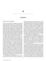
Particle Size Distribution On the basis of a sieve analysis
of fall diameter analysis, of a sediment sample, a cumulative
frequency curve for the particle size can be drawn. Figure 1

shows typical particle size frequency curves for a sample taken
from a sandy stream bed and for a sample of suspended load
over the same bed.
6
The frequency curves are usually plotted
on logarithmic-probability paper.
TABLE 1
Sediment grade scale
Group Particle size range, mm
Boulders 4096–256
Cobbles 256–64
Gravel 64–2
Sand 2–0.062
Silt 0.62–0.004

Clay 0.004–0.00024
FIGURE 1 Typical particle size frequencies curves for stream sediments (after Bishop et al.).
GRAIN SIZE (mm.)
IN TRANSPORT (by dunes)
PERCENT FINER (by weight)
ON THE
BED
1.0
.01 .05 .1 .2 .5 1 2 5 10 20 30 40 50 60 70 80 90 95 96 99 99.5 99.9 99.99
.10
.08
.20
.30
.40
.50.
.60
.80
C019_001_r03.indd 1065C019_001_r03.indd 1065 11/18/2005 11:05:59 AM11/18/2005 11:05:59 AM
© 2006 by Taylor & Francis Group, LLC
1066 SEDIMENT TRANSPORT AND EROSION
Some important descriptors of the frequency distribution
are: (1) the median size or d
50
, that is, the size for which 50%
by weight of the sample has smaller particles; (2) the scatter of
particle size as indicated, for example, by the standard devia-
tion or perhaps the geometric deviation; (3) the characteristic
grain roughness which has been associated with the d
65
;

5,7,8

(4) the d
35
has also been used as characteristic sediment size.
9

Bulk Properties The determination of bulk, in place
specific weights of sediments is discussed under Reservoir
Sedimentation.
EROSION
Most of the sediment in streams is produced by the following
processes:
1

1) Sheet erosion,
2) Gully erosion,
3) Stream channel erosion,
4) Mass movements of soil (e.g. landslides and soil
creep),
5) Erosion to construction works,
6) Solids wastes from municipal, industrial, agricul-
tural and mining activities.
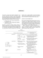
Morisawa,
10
using a system diagram, similar to Figure 2, sum-
marizes the inter-relation of climatic and geologic factors that
influence soil erosion and runoff. Figure 2 also shows man’s
influence on the system.
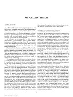
Langbein and Schumm

3,17
proposed the correlation
shown in Figure 3 between annual sediment yield and effec-
tive annual precipitation for the United States. The effec-
tive precipitation is the adjusted precipitation which would
have produced the observed runoff for an annual mean
temperature of 50°F.
A recent paper by Saxton et al.
11
relates total runoff, surface
runoff and land use practices to the sediment yield from loessial
watersheds in Iowa. This paper compares erosion and surface
runoff from contoured-corn watersheds and from pastured-
grass and level-terraced areas. In a 6-year study the contoured-
corn areas yielded, annually, about 19,000 tonsրsq. mile of
sheet erosion plus 3000 tonsրsq. mile of gully erosion while the
level terraced and grassed watersheds yielded about 600 tonsր
sq. mile. Similarly the surface runoff from the contoured-corn
areas was approximately 5 inches compared with 1.5 inches
for the level-terraced and grassed areas. The experimental
watersheds were of the order of 100 square miles.
Other land use factors are discussed in a paper by Dawdy
12

who presents sediment yields for the state of Maryland. The
annual sediment yield from heavily wooded areas is about
15 tonsրsq. mile compared with 200 to 900 for crop land.
The annual sediment yields from urban development areas
(usually only a few acres) varied from about 1000 to 140,000
tonsրsq. mile.

Curtis
13
obtained annual sediment yields of 390 and 290
for two watersheds (264 and 651 square miles) in the Miami
Conservancy District, Ohio.
A number of empirical formulae have been devel-
oped
1,14,15
to permit estimation of rates of overland erosion.
The US Department of Agriculture developed the universal
soil-loss equation (for upland areas),
E ϭ RKLSCP, (1)
where E ϭ soil lossրunit area; R ϭ rainfall runoff factor;
K ϭ soil erodibility factor; L ϭ slope length factor; S ϭ slope
steepness factor; C
1
ϭ crop management factor; and P
1
ϭ
erosion control practice factor. Details for estimating the
above factors are given by Meyer.
15

MEASUREMENT OF SEDIMENT DISCHARGE
Samplers have been developed to measure both suspended
and bed load in streams. However bed-load samplers are not
temp, rain
rock type topography
excavations
fills

reservoirs
CLIMATE
GEOLOGY
SOIL CHARACTER
SOIL EROSION
(RUNOFF)
RAINFALL
VEGETATION
MAN
farming
lumbering
amount
intensity
duration
MAN
eg.
eg.
FIGURE 2 The relationship of climate and geology to soil erosion (adapted from Morisawa).
C019_001_r03.indd 1066C019_001_r03.indd 1066 11/18/2005 11:05:59 AM11/18/2005 11:05:59 AM
© 2006 by Taylor & Francis Group, LLC
SEDIMENT TRANSPORT AND EROSION 1067
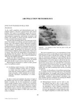
widely used because of their doubtful accuracy. Generally, only
suspended load samples are collected in samplers of the type
shown schematically in Figure 4.
This sampler is designed so
that the intake velocity is nearly the same as the local stream
velocity. The extent of the suspended sampled zone is limited
by the size of the sampler. Methods or extrapolating these
measurements and estimating bed load are discussed in the next
section.

For more details of sediment measurement techniques and
equipment, the reader is referred to Nordin and Richardson,
15

010
20 30
40
50
60
200
400
600
800
1000
EFFECTIVE PRECIPITATION (inches/year)
SEDIMENT YIELD (tons/sq.mi/year)
T = 50°F
FIGURE 3 Sediment yield in the United States (after Langbein and Schumm).
FLOW
AIR
WATER
SEAL
INTAKE
SAMPLE BOTTLE
SPRING
EXHAUST VENT
FIGURE 4 Sketch of a suspended load sampler.
C019_001_r03.indd 1067C019_001_r03.indd 1067 11/18/2005 11:05:59 AM11/18/2005 11:05:59 AM
© 2006 by Taylor & Francis Group, LLC
1068 SEDIMENT TRANSPORT AND EROSION

Shen,
15
Karaki,
15
Graf,
16
Brown,
1
Simons, and Senturk and
the ASCE Sedimentation Engineering Manual.
In some instances
15
turbulence flumes (a concrete lined
reach with baffles to create severe turbulence) have been con-
structed across a stream channel in order to suspend the bed
load and thus to sample it by suspended load techniques.
THE MECHANICS OF SEDIMENT TRANSPORT
IN A STREAM
General
The nature of sediment transport in a stream depends on the
shear intensity of the flow and the type of bed material. The
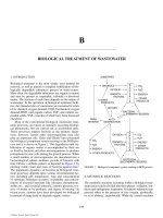
diagram in Figure 5 shows the sequence of bed forms (waves)
associated with increasing levels of shear on a fine granular
bed material.
3
This figure also shows, schematically, the typi-
cal changes in the Darcy friction factor and the sediment con-
centration with increasing flow velocity. The primary mode
of transport of particles, in the case of ripples,
17

is discrete
steps along the bed; however with increasing shear more of
the bed material becomes suspended until the particle motion
is nearly continuous for anti-dunes.
Dunes and ripples are triangular in shape with relative
flat upstream slopes and sleep downstream slopes. The
water surface waves are out of phase with the dune forma-
tion while ripple formations appear to be independent of the
free surface.
Dune wave lengths, ␭
d
, are related to the depth of flow
and in general,
l
d
Ͼ 3 feet (2)
whereas ripple wave lengths ␭
r
are shorter,
2" Շ l
r
Շ 18" (3)
Dune heights, H
d
, are related to the depth of flow, with the
limiting height approaching the average flow depth. The
ratio of dune length to height is given by
17

815ՇՇ
l
H
d
.
(4)
The maximum ripple height is about 0.1 feet.
Both ripples and dunes progress downstream. The tran-
sition from dunes to anti-dunes occurs at a Froude number
close to 1.0.
Anti-dunes, as indicated by Figure 5, are in phase with
the surface wave. The may be stationary or move upstream.
The maximum height of an anti-dune is approximately equal
to the flow depth at the trough of the surface wave.
Simons,
17,18
on the basis of experimental data, developed
the relationship shown in Figure 6 between stream power and
bedform for varying fall diameters. Simons and Richardson
19

also studied the variation of Chézy’s C with bed form. Their
results are summarized in Table 2.
0
12
34
56
V feet/sec.
Friction
Factor

f
0.02
0.04
0.06
0.08
0.1
1
10
100
1,000
10,000
100,000
Concentration of
Bed Material
C ppm.
Flat
Bed
Ripples Dunes Transition Antidunes
C
f
FIGURE 5 The behavior of a mobile stream bed (adapted from Leopold, Wolman, and Miller).
C019_001_r03.indd 1068C019_001_r03.indd 1068 11/18/2005 11:06:00 AM11/18/2005 11:06:00 AM
© 2006 by Taylor & Francis Group, LLC
SEDIMENT TRANSPORT AND EROSION 1069
Initial Motion
White, in 1940,
20,21
using an analytical approach, showed
that, for sufficiently turbulent flow over a granular bed, the
critical shear or shear to initiate grain movement is

t
c
ϭ k
c
g
f

( S
s
–1) d, (5)
in which k
c
; 0.06; g
f
ϭ fluid specific weight; S
s
ϭ specific
gravity of sediment grain; d ϭ grain diameter.
Shields,
21
using an experimental approach, obtained the
more general equation
t
c
ϭ g


f

( S
s
–1) d f ( R
*
), (6)
in which R
*
ϭ U
*
dր n; U
*
ϭ friction velocity; n ϭ kinematic
viscosity; and f ( R
*
) is defined in Figure 7.
Permissible or allowable tractive stresses for use in chan-
nel designs with granular or cohesive boundaries are given
by Chow.
7

Bed Load Formulae
When the bed shear, t
o
, due to the flowing stream exceeds the
critical shear, t
c
, a part of the bed material starts to move in a
layer of the stream near the bed, i.e. the bed layer. Experimental
0.2
0.4

0.6
0.8 1.0
1.2
0
Median Fall Diameter in mm.
0.001
0.002
0.004
0.006
0.008
0.01
0.02
0.04
0.06
0.08
0.1
0.1
0.2
0.4
0.6
0.8
1.0
1.0
10
4.0
2.0
Stream power, tV, lbs/ft – sec.
Stream power, tV, gms/cm – sec.
Upper Region
Transition

Dunes
Ripples
Plane
FIGURE 6 Relation of stream power and median fall diameter to bed form (after
Simons).
TABLE 2
Chézy C in sand channels
Regime Bed Form
Cl √g (where C is Chézy C)
Lower regime
ripples d
50
Ͻ 0.6 mm 7.8 to 12.4
dunes 7.0 to 13.2
transition 7.0 to 20
Upper regime plane bed 16.3 to 20
anti-dune {standing wave 15.1 to 20
{breaking wavechutes and
pools“slug” flow
10.8 to 16.3
9.4 to 10.7
—
C019_001_r03.indd 1069C019_001_r03.indd 1069 11/18/2005 11:06:00 AM11/18/2005 11:06:00 AM
© 2006 by Taylor & Francis Group, LLC
1070 SEDIMENT TRANSPORT AND EROSION
studies
3
indicate that this sediment discharge, known as the
bed load, q
B

, is a function of the excess of t
o
above t
c
or
q
B
ϰ fcn ( t
o
— t
c
). (7)
Figure 8 illustrates a typical experimental relationship
between q
B
and ( t
o
— t
c
).
DuBoys in 1879
22
treated the bed material, involved
in the bed load, as it if consisted of sliding layers which
respond to and distribute the applied stress t
o
. He proposed
the relation
q
B

ϭ C
s
t
o
( t
o
– t
c
) (8)
Both C
s
and t
c
depend on particle size as indicated in Table 3.
Chang,
1
Schoklitsch,
1,16
MacDougall,
1
and Shields
1
have
presented bed load formulae similar to Eq. (8).
The theoretical bed load model developed by Einstein
4,5,8,24

has formed the basis for a number of researches in sediment
transport.
6,15,24,36

Einstein utilized: (1) the statistical nature of
turbulent flow; (2) the fact that in steady uniform flow there
is an equilibrium between the processes of erosion and depo-
sition, that is, (probability of erosion) ϭ (the probability of
deposition); (3) the fact that grains near the bed are more in
quick “steps” interrupted by “rest” periods; (4) a separate
hydraulic radius, R ′, associated with grain roughness and
another hydraulic radius, R ′′, associated with the bed form.
Einstein obtained the erosion probability function by
assuming that the lift force, on a grain, consists of an aver-
age component [related to ( U
*
)
2
] and a normally distributed
random component. Einstein thus obtained the “bed load”
equation

A
A
t
B
B
o
o
∗∗
∗∗
−−
−
∗∗

∗∗
∫
⌽
⌽1
1
1
1
ϩ
ϭ
p
ch
ch
d
(/ )
(/ )

(9)
in which

⌽ϭ
Ϫ
∗
iq
igdS
BB
bs s
g
3
1()

(10)
is Einstein’s bed transport function; A
*
ϭ 43.5; B
*
ϭ 0.143;
h
o
ϭ 1ր2;

cj
∗
⎧
⎨
⎪
⎩
⎪
⎫
⎬
⎪
⎭
⎪
ϭ
⌬
Ϫ
ϪЈ
Y
X
S
d

SR
s
log
log
.
()
10.6
2
10 6
1

(11)
in the Einstein flow intensity function; i
B
ϭ fraction of q
B
in the
size range associated with d; d ϭ geometric mean of particle
1.0
0.01
0.1
1.0
10
100 1000
R
s
=
U
s
f

n
f(R
s
)
Laminar
flow of bed
Turbient
flow of bed
FIGURE 7 Shields’ critical shear function (adapted from
Henderson).
0.001
0.003
0.005
0.007 0.009 0.011
0.013
0.0
0.02
0.03
0.04
0.05
0.06
0.07
0.08
0.09
0.10
0.11
0.12
0.13
0.14
0.15

0.01
T
0
(gm/cm
2
)
SEDIMENT LOAD (gm./sec./cm.)
T
0
FIGURE 8 Typical relation of shear and sediment load
(adapted from Leopold, Wolman and Miller).
TABLE 3
Typical values of C
s
and t
c
(after Straub
22,23
)
d mm
1
8
1
4
1
2
124
C
s
ft

6
2
16 Ϫsec
0.81 0.48 0.29 0.17 0.10 0.06
t
c
lb
ft
2
0.016 0.017 0.022 0.032 0.051 0.09
C019_001_r03.indd 1070C019_001_r03.indd 1070 11/18/2005 11:06:00 AM11/18/2005 11:06:00 AM
© 2006 by Taylor & Francis Group, LLC
SEDIMENT TRANSPORT AND EROSION 1071
size range being considered; S
e
ϭ energy slope; i
b
ϭ fraction
of bed sediment in specified range; j ϭ hiding factor; Y ϭ lift
correction factor; ⌬ ϭ d
65
ր X; X ϭ correction factor for hydrau-
lically smooth flow; dЈ ϭ 11.6 n ր U
*
;

UgRS
e
ЈϭЈ
∗ (12)

X ϭ 0.770 if ⌬ր d Ͼ 1.80; X ϭ 1.39 d if ⌬ր d Ͻ 1.80.
Schen
15
gives an up-to-date review of the modern stochas-
tic approaches to the bed material transport problem.
The Suspended Load
Equations of Motion of the Fluid The flow in natural streams
is almost always turbulent and may be assumed to be incom-
pressible; consequently the applicable equations of motion
for the fluid are the Reynolds
25
equations

rs
∂
∂
∂
∂
⎡
⎣
⎢
⎢
⎤
⎦
⎥
⎥
∂
∂
U
t

U
U
xx
F
i
j
i
jj
ji
i
ϩϭ() ,ϩ

(13)
in which U
_
i
ϭ ensemble mean point velocity in the direction i;
s
ij
ϭ stress tensor ϭ{ϪP
_
d
ji
ϩmD
_
ji
Ϫru
i
u
j

} ϭ average pressure;
d
ji
ϭ Kronecker delta; m ϭ dynamic viscosity; D
_

ji

ϭ deforma-
tion tensor; Ϫ ru
i
u
j
ϭ turbulence or Reynolds Stresses; r ϭ
fluid density ; u
i
ϭ random component of velocity in the i
direction; F
_
ϭ body force in the i direction. The first term in
the stress tensor represents the normal stresses due to the aver-
age pressure at a point; the second term represents the viscous
shear forces; the last term or Reynolds stress has both normal
and tangential components. A common method of simplify-
ing equations involves the introduction of an eddy viscosity,
␧
m
such that

rr␧ϭϪ

m
ji
i
jji
Duu
()
.
≠
(14)
The requirement that ( i  j ) in Eq. (14) eliminates the normal
stresses due to turbulence; in order to account for these
normal stresses an average turbulence pressure P
_
i
is added to
P
_

thus yielding the simplified stress tensor

sdmr
ji
t
ji m i ji
PP DϭϪϩϩϩ␧()( ).

(15)
The fluid continuity equation is

∂

∂
U
x
i
i
ϭ 0. (16)
Equations (13), (15), and (16) may be solved in a few
cases by methods developed to solve the Navier-Stokes
equations.
Transport of a Scalar Quantity in Turbulent Flow In an
incompressible turbulent fluid the conservation of a scalar
quantity requires that the rate of change of a scalar (say

c
_

plus the rate of generation of c
_

at the point or

Dc
Dt x
h
c
x
uc F
ii
i
c

ϭϪЈϩ
∂
∂
∂
∂
⎛
⎝
⎜
⎞
⎠
⎟ (17)
in which c ϭ c
_
ϩcЈ; c
_
ϭ ensemble average of c; c Ј ϭ random
component of c; D ր Dt ϭ substantial derivative; F
_
c_
is the gen-
eration term; h ϭ molecular diffusion coefficient. It is usual
to introduce, into Eq. (17), an “eddy” transport coefficient
␧
j
, such that

ϪЈϭ␧uc
c
x
ic

i
∂
∂
.

(18)
Since in most practical problems ␧
c
ϾϾ h, then Eq. (17) can
be reduced to

Dc
tx
c
x
F
i
c
i
c
d
ϭ␧ϩ
∂
∂
∂
∂
⎛
⎝
⎜
⎞

⎠
⎟
.

(19)
Equations (3) and (19) are valid for low sediment
concentrations. A review paper by Vasiliev
26
discusses the
governing equation which account for various levels of sedi-
ment concentrations. For example a first order correction to
the Reynolds equations is

rs
DU
Dt x
rc F
i
i
ji t
ϭϩϩ
∂
∂
()( ).1

(20)
The volume continuity equation is the same as Eq. (16) while
the mass continuity equation becomes

Dc

Dt x
cu v
c
x
i
is
ϭϪϩ
∂
∂
∂
∂
⎧
⎨
⎩
⎫
⎬
⎭
()
3
(21)
in which r ϭ ( S
s
—1); c
_

ϭ average ensemble concentration
at a point (massրmass); n
s
ϭ settling viscosity; x
3

ϭ vertical
coordinate (opposite to the direction of n
s
).
The Vertical Concentration Profile There is no general solu-
tion for Eqs. (3), (16), and (19) or (18), (20), and (21); however
a few special cases, of practical interest, have been solved.
Using the simplifications which result for steady, uni-
form flow in two dimensions (as shown in Figures 9 and 10),
it is possible to obtain a solution for the vertical velocity, and
concentration profiles. The following assumptions are typi-
cal of those required to solve Eqs. (13), (14), and (21):
a) c
_



ϾϾ 1;
b) ␧
c
ϭ b␧
m
where b ; 1;
c) F
_
x
; grs
0
;
C019_001_r03.indd 1071C019_001_r03.indd 1071 11/18/2005 11:06:00 AM11/18/2005 11:06:00 AM

© 2006 by Taylor & Francis Group, LLC
1072 SEDIMENT TRANSPORT AND EROSION
d)

∂
∂
()
;
PP
x
t
ϩ
ϭ 0

e)

tr tro g and g );ϭϭSoD So (D yϪ

Chang et al. , used the above assumptions to obtain: (a) the
vertical velocity profile,

U
U
U
xx
ϭϪ␧Ϫ
␧
ϪϪ␧
ϩϩ
2

1
11
1
3
12
*
/
k
1n
⎛
⎝
⎜
⎞
⎠
⎟
⎧
⎨
⎪
⎩
⎪
⎫
⎬
⎪
⎭
⎪
(22)
and (b) the vertical concentration profile

cy c
a

y
a
DDa
DDy
z
() ,
/
ϭ
Ϫ
Ϫ
⎛
⎝
⎜
⎞
⎠
⎟
−
()
−
()
⎧
⎨
⎪
⎩
⎪
⎫
⎬
⎪
⎭
⎪

12
2

(23)
in which U
*
ϭ friction velocity
ϭ gDs
0
;

␬ϭ fcn ( U
*
d ր v ) Ϭ 0.4;
␧ ϭ y ր D; Ú ϭ average velocity in vertical; a ϭ reference height;
Z ϭ v
s
ր( bU
*
k ). Using the Keulegan velocity distributions

U
yU
v
x
ϭ 575
905
10
.log
.

∗
⎛
⎝
⎜
⎞
⎠
⎟

(for smooth boundaries) (24a)
U
y
d
x
ϭ 575
30 2
10
65
.log
.
⎛
⎝
⎜
⎞
⎠
⎟

(for smooth boundaries) (24b)
Einstein and others
5,1
have obtained a slightly different equa-

tion for c ( y ), i.e.

cy c
a
aD y
yD a
z
() .
()
()
ϭ
−
−
⎡
⎣
⎢
⎤
⎦
⎥
(25)
The Suspended Sediment Load The suspended sediment dis-
charge q
s
(weightրunit timeրunit width) above a reference
level y ϭ a is given by

qUcdy
s
x
a

D
ϭg
∫
,

(26)
where U
–
and c
–
are given by Eqs. (22) and (23) or (24) and (25).
Longitudinal Dispersion Another problem which has
received some attention is that of longitudinal diffusion and
dispersion in natural streams and estuaries. Several research-
ers
16,33,34,35
have sought analytical and numerical solutions for
the longitudinal variation in the mean concentration in the
vertical, c
–
.
Considering two dimensional longitudinal dispersion,
Eq. (17) can be approximated by
16


∂
∂
∂
∂

∂
∂
ˆˆ ˆ
c
t
U
c
t
E
c
x
x
L
ϩϭ
2
2
(27)
in which E
L
; coefficient of longitudinal diffusion. A typical
16

value for E
L
is

EUD
L
ϭ 59
∗

The solution of Eq. (27) for an initial step change, M
o
, in
concentration, is

ˆ
(,) .
()/
cxt
M
Et
e
o
L
xUt Et
xL
=
−−
4
2
4
p
(29)
Other treatments of the dispersion problem may be found in the
works of Holley
28
Householder et al. ,
29
Chiu et al. ,

30
Conover
et al. ,
31
Sooky,
32
Fischer,
33
Harleman et al. ,
34
and Sayre.
35

The Total Sediment Load
Einstein
5
developed a unified total bed material formulae by
converting his computed bed load, q
B
to a reference concen-
tration

at y ϭ a ϭ 2 d. Inserting

into Eqs. (25) and (26) he
obtained an estimate of q
sB
the suspended bed material load.
Hence the total bed material load per unit width, q
TB

is
q
TB
ϭ q
B
ϩ q
sB

ϭ ⌺ i
B
q
B
(1 ϩ P
e
I
1
ϩ I
2
) (30)
all size
ranges
S
0
FLOW
T
0
=gDS
0
g(D–y)S
0

1
y
y
D
T
FIGURE 9 Defining sketch for uniform flow.
D
U
x
U
x
C
σ
C
y
S
0
σ
FIGURE 10 Defining sketch for velocity
and concentration profiles.
C019_001_r03.indd 1072C019_001_r03.indd 1072 11/18/2005 11:06:01 AM11/18/2005 11:06:01 AM
© 2006 by Taylor & Francis Group, LLC
SEDIMENT TRANSPORT AND EROSION 1073
in which

I
Ky yIKy
z
AA
ee

1
1
2
1
11 11ϭϪϭϪ(); ();/d /lnd
∫∫
y y

K ϭ
0.216


AA
e
Z
e
Z′′Ϫ
Ϫ
1
1/( ) ;

A
e
ϭ 2dր D ; P
e
ϭ 2.3 log 30.2 ␹d ր d
65
;
Z ′ ϭ v
s

ր( bU
*
␬ ); ( X see Bed Load Formulae ).
The total sediment load per unit width in a stream q
T
is
q
T
ϭ q
TB
ϩ q
w
, (31)
where q
w
ϭ wash load (fines) which must be obtained inde-
pendently, e.g. by direct measurement. The Einstein method
requires a knowledge of: grain size distribution in the bed;
the grain density; the energy slope, S
e
; and the water temper-
ature, in order to compute both bed material load and water
discharge for a given depth and width of flow.
Colby and Hembree
9,36
modified Einstein’s method in
order to compute total sediment load ( q
T
). Their procedure
utilizes: the sampled suspended load Q

s
; measured discharge;
measured depths and sampler depths, the extent of the sam-
pled zone; and all the data used by the Einstein procedure
except S
e
. Their main modifications are:
1) The finer portion of the total suspended load, Q
s
,
is based on extrapolation of the actual sampled
load Q′
s
(using Eqs. (25) and (26)).
2) The coarser part of the total load (including the
bed load) is computed from a simplified Einstein
procedure (using a modification of Eq. (30)).
3) Einstein’s grain shear velocity U′∗ is replaced
by an equivalent shear velocity U
m
based on the
Keulegan equations and the measured discharge.
4) Einstein’s flow intensity function ␺
*
, is replaced
by the larger of
C
m
ϭ 1.65 gd
35

ր( U
m
)
2
or C
m
ϭ 0.66 gd ր( U
m
)
2
(32)
5) The modified term ⌽
m
is used to enter Einstein’s
Eq. (9) to obtain a bed transport function ␺
*
; the
modified bed transport function is
⌽
*
ϭ ⌽
*
ր2. (33)
The value of ⌽


m


is used to compute the bed load associated

with a size range d, i.e.
i
B
q
B
; 1200 d
3 ր2
i
B
⌽


m


lbրsecրft. (34)
6) Using the computed bed load for a certain size
range, i
B
Q
B
, the measured suspended load in the
same size range, I
s
Q′
s
,

and Einstein’s Eq. (30) one
can obtain a value for Z ′ in Eq. (25) which should

be better than a Z ′ based on an estimated v
s
.
Bishop, Simons, and Richardson
6
simplified the Einstein
procedure for determining total bed material load. They
introduced a single sediment transport function ⌽

T

which
includes both suspended bed material and bed load. Their
flow intensity term is

y
Ts
e
S
d
RS
=−
′
().1
35
(35)
The experimental relationship shown in Figure 11
were estab-
lished for actual river sediments of various median sizes. Using
⌽

T

from Figure 11 the total bed material load per unit width, is
q
TB
= ⌽
Trs
(gd)
3/2
(S
s
–1)
1/2
. (36)
The wash load must be added to q
TB
to obtain the total
sediment load.
Colby
37
analysed extension laboratory and field data to
establish the empirical relationship, shown in Figure 12, for
the determination of sand discharge. Figure 12 is valid for a
water temperature of 60°F and a flow to moderate wash load
(c
^
<10,000 ppm). Colby provides adjustment coefficients for
water temperature and wash load. For example, at a flow
depth of 10 feet a Ϯ20°F change in temperature would result

in about ϩ25% change in the sand discharge and an increase
in the concentration of fines from 0 to 100,000 ppm could
cause up to 10 fold increase in the sand load.
The reader is referred to Graf,
16
Shen,
15
and Chang et al. ,
27

for other contributions to the determination of total bed
material load.
The Annual Sediment Transport
In general it is not practical to continuously sample the sedi-
ment in a stream; instead, representative samples are taken
for various flow conditions and a sediment load versus water
discharge or sediment rating curve is established. A typical
sediment rating curve is shown in Figure 13. A number of
factors contribute to the scatter of data points in Figure 13.
The sediment load is out of phase with the discharge hydro-
graph as illustrated by Figure 14. The sediment load depends
on the season of the year.
Using the available stream flows and the sediment
rating curve an average annual sediment transport can be
estimated.
Often the bed load is not included in the sediment rating
curve; if this is the case, the bed load may be computed as
discussed under Bed Load Formulae and added to the annual
sediment transport.
THE RESPONSE OF A CHANNEL TO CHANGES IN

ITS SEDIMENT CHARACTERISTICS
Lane’s Model
Lane
39
proposed the relationship
(sediment load) ϫ (sediment size) ϱ (stream slope) ϫ
(stream flow)
or
( Q
s
ϫ d ) ϱ ( S ϫ Q ) (37)
to describe qualitatively to behavior of a stream carrying
sediment.
Lane used the following terms in referring to streams:
(1) “grade ϵ equilibrium or regime slope; (2) “aggrad-
ing” ϵ rising of the stream bed due to deposition;
(3) “degrading” ϵ losing of the stream bed due to scouring
C019_001_r03.indd 1073C019_001_r03.indd 1073 11/18/2005 11:06:01 AM11/18/2005 11:06:01 AM
© 2006 by Taylor & Francis Group, LLC
1074 SEDIMENT TRANSPORT AND EROSION
(4) “base level” ϵ the local level to which a stream tends to
cut its bed.
Lane contended that there is a natural tendency for a bal-
ance between the products in Eq. (38). For example, if one
of the factors, Q
s
, is decreased then, in order to balance the
equation, the stream slope might also tend to decrease, i.e.
degradation. On the other hand an increase in Q
s

could lead
to an increase in S, i.e. aggradation.
The Regime Approach
“The dimensions (width, depth, and slope) of a channel
to carry a given discharge, with a given silt load, are fixed by
nature, i.e. uniquely determined.” A channel whose dimen-
sions are so established is said to be in regime.
In the geological sense
3,10
a river system is never really
in equilibrium. According to W.M. Davis, who postulated a
geomorphological cycle,
3,10
the agents of uplift and gravity
(represented mainly by steam erosion) are always opposing
each other. However, from the engineering point of view, a
stream can be considered to be in “equilibrium” over a period
of a few decades if its average behavior or average dimen-
sions remain unchanged. There are always fluctuations, of
the channel geometry, about this average; thus the steam is
sometimes said to be in “dynamic equilibrium.”
Of course, a stream may be aggrading or degrading (on
the average in Engineering time) and thus it is not in equi-
librium. The regime theory could be used to predict the ulti-
mate dimensions of a stream that is not in regime.
Kennedy
40
and Lindley
41
collected data from canals in

India (Pakistan) and proposed an equation for the non-filtering,
non-scouring velocity, v,
v ϭ C
1
y
n
, (38)
where C
1
ϭ 0.84; n ϭ 0.64; and y ϭ depth of flow.
Kennedy was followed by Lacey, Inglis, and Blench who
developed equations for channel slope and width.
Lacey
42,21
introduced the equations

vfR= 117.

(39)
0.93 mm.
0.47 mm.
0.19 mm.sand
0.27 mm.
.0001
.001
.01
.1
1
10
100

1000
.2 .4
.6
.8 1.0 2
4
610
20
40 60 80
␺
T
␾
T
FIGURE 11 Bed material transport function (after Bishop et al.).
C019_001_r03.indd 1074C019_001_r03.indd 1074 11/18/2005 11:06:01 AM11/18/2005 11:06:01 AM
© 2006 by Taylor & Francis Group, LLC
SEDIMENT TRANSPORT AND EROSION 1075

fd= 8

(40)
v ϭ 16 R
2 ր3
S
1 ր3
(41)

PQ= 267.
(42)
in which R ϭ hydraulic radius (ft.); d ϭ medium grain diam-
eter (inches); P ϭ wetted perimeter (ft.) Q ϭ dominant dis-

charge ϭ ␷PR (cfs.).
The dominant discharge in the case of canal flow is the
design flow. In the case of a natural stream it is the channel
forming flow which is often taken to be the bankfull dis-
charge
3
which has an approximate return period of, between
1.25 and 2.33, years.
Blench
43
advanced the work of Lacey and introduced
bed and side factors to better describe the depth and width of
a channel in regime. His equations are:
f
b
ϭ v
2
ր y ϭ bed factor (43)
f
s
ϭ v
3
ր b ϭ side factor (44)
and

S
ff
gQ c
bs
=

+
() ()
.(/)
,
///
/
56 112 14
16
1
3 63 1 2330
(45)
in which c is the concentration in ppm; b ϭ mean width
(ft—sec. units). The recommended f
b
is

fd c
b
=+9 6 1 0 012.()(. )in

(46)
1 2 4 6 1.0 2 4 6 1.0 2 4 6 1.0 2 4 6 1.0
MEAN VELOCITY ft/sec
0.1
1
10
100
1000
10,000
DISCHARGE OF SANDS, tons/day/foot of width

DEPTH
0.1 ft
DEPTH
1.0 ft
DEPTH
10 ft
DEPTH
100 ft
Sand Size
0.1 m.m.
0.2
0.4
0.8
FIGURE 12 Sand discharge (after Colby).
C019_001_r03.indd 1075C019_001_r03.indd 1075 11/18/2005 11:06:01 AM11/18/2005 11:06:01 AM
© 2006 by Taylor & Francis Group, LLC
1076 SEDIMENT TRANSPORT AND EROSION
and f
s
depends on the cohesiveness of the material in the
channel banks. For example, f
s
is approximately 0.1, 0.2, and
0.3 for low, medium, and high cohesiveness respectively.
The data of Lacey and Blench were mainly from canals,
with moderate to low sediment loads ( c Ͻ 500 ppm) and
with sand beds and slightly cohesive banks.
17

Simons and Albertson

44,21
have extended the regime
equations to make them applicable to the five channel clas-
sifications shown in Table 4.
They proposed the following general equations:
P ϭ K
1
Q
1 ր2
(47)
10
1
10
1
10
2
10
2
10
4
10
4
10
5
10
6
10
3
10
3

SEDIMENT LOAD (tons/day)
MEAN DAILY DISCHARGE (cfs)
SUMMER STORMS AND
WINTER RUNOFF
SNOW RUNOFF
FIGURE 13 Typical sediment rating curve (adapted from Ref. 38).
Q
Qs
Q
t
SUSPENDED
SEDIMENT
LOAD
Qs
DISCHARGE
FIGURE 14 Variation of sediment load with time (adapted from Graf).
C019_001_r03.indd 1076C019_001_r03.indd 1076 11/18/2005 11:06:02 AM11/18/2005 11:06:02 AM
© 2006 by Taylor & Francis Group, LLC
SEDIMENT TRANSPORT AND EROSION 1077
b ϭ 0.9 P (48)
b ϭ 0.92 B –2.0 (49)
R ϭ K
2
Q
0.36
(50)
y ϭ 1.21 R for R Ͻ 7 ft. (51)
y ϭ 2 ϩ 0.93 R for R Ͼ 7 ft. (52)
v ϭ K
3

( R
2
S )


m


(53)

C
g
v
gyS
K
vb
v
22
4
037
ϭ=
⎛
⎝
⎜
⎞
⎠
⎟
.

(54)

in which C ϭ Chézy coefficient; B ϭ surface width; the
values of the K ’s and m are defined in Table 5.
Schumm
17,45
studied the Great Plains rivers in the US
and similar rivers in Australia; he correlated stream geom-
etry with discharge (mean annual flood Q
ma
) and the percent
silt-clay, M, in the channel boundary. Some of his correla-
tions are:

Full Bank width ϭ W ϭ
23
058
037
.
()
.
.
Q
M
ma

(55)

Width: depth ratio
ϭϭ
W
D

Q
M
ma
21
018
074
.
.
()
(56)
Sinuosity ϭ 0.94 M
0.25
, (57)
The high correlation of stream geometry and M led
Schumm to classify channels (see Table 6) using M as an
index to the ratio of coarse load to total load.
Schumm
45,17
associated meandering channels with high
values of M and low bed load and braided channels (a relatively
straight, steep main channel consisting of a maze of sub-channels
sometimes separated by bars or islands) with low values of M
and high bed load.
RESERVOIR SEDIMENTATION
A common objective of many sediment transport studies is
the prediction of reservoir “siltation” rates. Reservoir siltation
depends on: (1) the average annual sediment load entering
the reservoir; (2) the grain size distribution of the sediment
load; (3) the reservoir trap efficiency; (4) the bulk dry specific
weight of the deposited sediments in the reservoir.

The determination of annual sediment yields was dis-
cussed in Sections Erosion and The Mechanics of Sediment
Transport in a Stream. It is important to predict the possible
effects of land development andրor sediment control mea-
sures on future sediment yields.
46

An estimate of the percentage sand, silt, and clay for the
incoming sediment can be obtained on the basis of grain size
analyses of the existing load.
Brune in 1953
47,8
presented the trap efficiency curve
shown in Figure 15,
which applies to reservoirs which nor-
mally ponded. Detention type reservoirs would have lower
trap efficiencies.
Since annual sediment yield is usually determined in terms
of weight it is necessary to know the bulk dry specific weight,
and the trapped sediments, in order to estimate the volumet-
ric decrease in reservoir storage. To accomplish this Lane and
Koelzer
48,8
developed an equation to describe the change in bulk
dry specific weight, ␥

* , of reservoir deposits with time, i.e.

gg
g

*()
*
()
*
( log )
( log )
ϭϩ
ϩϩ
sand sand sand
silt silt si
110
110
KTX
KTX
llt
cla clay clay
ϩϩ( log )
()
*
g
y
KTX
110


(58)
in which T ϭ time in years; X
sand
ϭ fraction of sand in deposit;
␥

*
sand(1)
etc. are the respective bulk dry specific weights at T р
1 year (see Table 7); K
sand
etc. are constants (see Table 7).
After a period of N years a reservoir will contain depos-
its varying in age from less than one year to N years with
the consequence that the true bulk dry specific weight, ␥

*

,
for the entire deposit should be found by averaging Eq. (58)
TABLE 4
Canal classification
21,44
1) Sand bed and banks.
2) Sand bed and cohesive banks.
3) Cohesive bed and banks.
4) Coarse noncohesive material.
5) Same as for 2, but with heavy sediment loads, 2000–8000 ppm.
TABLE 5
Constants in Eqs. (47) to (54) (ft-sec. units)
Coefficient
Channel type
1234 5
K
1

3.5 2.6 2.2 1.75 1.7
K
2
0.52 0.44 0.37 0.23 0.34
K
3
13.9 16.0 — 17.9 16.0
K
4
0.33 0.54 0.87 — —
m
0.33 0.33 — 0.29 0.29
TABLE 6
Schumm’s classification
Stream type Bed load Mixed load Suspended load
M Braided Meandering
Ͼ 5% 5–20% > 20%
Coarse load
Total total
Ͼ 11% 3–11% < 3%
C019_001_r03.indd 1077C019_001_r03.indd 1077 11/18/2005 11:06:02 AM11/18/2005 11:06:02 AM
© 2006 by Taylor & Francis Group, LLC
1078 SEDIMENT TRANSPORT AND EROSION
over the N year period. Some typical
8
averaged values of
␥
–
*
for various time periods are:

N ϭ 10 years,

gg
**
.
10 1
0 675=
=T
Kϩ

N ϭ 50 years,
gg
**
.
50 1
1 298ϭϩ
T
K
=

N ϭ 100 years,
gg
**

100 1
1 588ϭϩ
T
K
=

The decrease in storage (in acre-ft) during an N year
period is given by:

⌬vϭ
ϫ
ϫ
TE SY DA N
N
100
2000
43 560
⎛
⎝
⎜
⎞
⎠
⎟
⎛
⎝
⎜
⎞
⎠
⎟
()( )
,
*
g

(59)

in which
TE
__
ϭ average trap efficiency in percent;
SY
—
ϭ average annual sediment yields in tonsրsq. mile;
( DA ) ϭ drainage area in sq. miles;
␥
–
*

N
ϭ average bulk specific weight for the N -year com-
putation period in lbsրft
3
.
A typical distribution of reservoir sediments is shown in
Figure 16. The coarse sediments (sands and gravels) form a
delta at the upstream section of the pond. Finer sediments
are deposited downstream from the delta. Very fine sediment
(clay particles) may pass through the reservoir or be depos-
ited in the downstream portion of the pond.
THE DEGRADATION PROBLEM
The response of a stream to changes in its sediment load was
described qualitatively in Section 6. The problem of comput-
ing the probable rate and extent of degradation downstream
from a proposed reservoir has recently received the attention
of a number of researchers.
15,49,50

Numerical estimates of the degrading channel profiles
may be obtained by solving, simultaneously, the following
equations (see Gessler, Ref. 15):
1) the equation of sediment continuity—

∂
∂
+
−
∂
∂
=
z
tb m
qb
x
TB
1
1
0
()
()
(60)
2) the bed material transport equation which may
have the form—
q
TB
ϭ C ′ ( ␶
o

– ␶
c
)

P

(61)
3) the bed shear equation—
␶
o
ϭ ␥RS
e
(62)
4) a friction equation, e.g. the Chézy equation—
v ϭ C ( RS
e
)
1 ր2
, (63)
0.001
0.01
0.1
1.0
10.0
0
20
40
60
80
100

CAPACITY-INFLOW RATIO (cap.acre ft./acre ft. annual inflow)
SEDIMENT TRAPPED %
ENVELOPE CURVES FOR NORMAL
PONDED RESERVOIR
MEDIAN CURVE FOR NORMAL
PONDED RESERVOIR
FIGURE 15 Trap efficiency curve (after Brune).
TABLE 7
Constants for Eq. (59) (after Lane and Koelzer)
Reservoir operation Sand Silt Clay
g*Kg*Kg*K
Normally submerged 93 0 65 5.7 30 16.0
Moderate reservoir drawdown 93 0 74 2.7 46 10.7
Considerable reservoir
drawdown
93 0 79 1.0 60 6.0
Reservoir normally empty 93 0 82 0.0 78 0.0
C019_001_r03.indd 1078C019_001_r03.indd 1078 11/18/2005 11:06:02 AM11/18/2005 11:06:02 AM
© 2006 by Taylor & Francis Group, LLC
SEDIMENT TRANSPORT AND EROSION 1079
in which z ϭ bed elevation; q

TB

ϭ volumetric bed material
load; m ϭ bed porosity; C ′ and p are constants for a given
bed material and bed form.
As the bed is soured, an armouring process occurs due to
the fact that the finer bed material is more readily removed
than the coarser particles in the bed (See Figure 1). This may

be accounted for by adjusting ␶
c
in Eq. (62).
SEDIMENT CONTROL
The adverse effects of excessive sediment loads in reser-
voirs, navigation channels, harbors, and aquatic life may be
alleviated by a sediment control program which may include
measures such as prevention of over-hand erosion or con-
tainment of eroded soil near its source. On the other hand
the removal of an established sediment load from a stream
may also lead to undesirable consequences such as channel
degradation or changes in the established aquatic life.
2

The ASCE Sedimentation Tank Committee
46
has clas-
sified sediment control measures under: (1) land treatment,
(2) structural.
Land treatment measures are used to reduce wash load
(fines) resulting mainly from sheet erosion. Structural mea-
sures are most effective for reducing sediment load derived
from stream-channel erosion, gully erosion, and sediment
associated with mining and construction work.
The main land treatment measures are summarized
below:
46

1) Vegetative treatment includes changes in the exist-
ing land use towards more: use of cover crops and

crop rotation, maintenance of effective vegeta-
tive cover in critical areas, leaving of straw and
stubble in the field, use of long-term hay stands,
mulching, pasture planting, and re-forestation.
2) Protecting existing vegetative cover involves pro-
tection of existing forest sands from excessive fire
losses and the protection of all vegetated areas
from over grazing.
3) Mechanical field practices are used in conjunc-
tion with (1) and (2) and include contour farm-
ing, contour furrowing of range land, contour
strip-cropping, use of gradient and level terraces,
use of diversions to divert runoff away from crit-
ical areas, use of grassed waterways and ditch
and canal linings, and the use of grade stabiliza-
tion structures in areas subject to possible gully
erosion.
The ASCE Task Committee
46
outlined three commonly
used structure measures:
1) Reservoirs, either detention or multi-purpose,
decrease flood stages and consequently may
decrease downstream damages due to deposition
of flood borne sediments; however it should be
remembered that reservoirs themselves create
sediment problems which may be just as serious
as the problem being solved.
2) Stream channel improvement and stabilization —
these measures may include straightening, clean-

ing, deepening, and widening of existing channels
in order to decrease local flood stages and related
sediment damages; again, complications, such
as increased channel erosion, can be expected.
Other channel improvement methods are: lining
the channel on bends and other erodible areas,
and providing spur dykes to deflect the flow away
from erodible banks.
3) Debris and sedimentation basins are usually rela-
tively small reservoirs designed to trap debris and
sediment near its source. This method is particu-
larly useful in controlling sediment yields from
construction sites or mining operations.
MILES
DAM
DEGRADATION
CLAYS
FEET
DENSITY
CURRENT
SILTS
DELTA
GRAVELS
SANDS
FIGURE 16 Distribution of deposits in a reservoir.
C019_001_r03.indd 1079C019_001_r03.indd 1079 11/18/2005 11:06:02 AM11/18/2005 11:06:02 AM
© 2006 by Taylor & Francis Group, LLC
1080 SEDIMENT TRANSPORT AND EROSION
LIST OF SYMBOLS
a ϭ 2 d ϭ reference distance from the stream bed;

A ϭ flow area;
A
e
ϭ aրD;
b ϭ average channel width;
B ϭ top width of channel;
c ϭ point concentration;
c
–
ϭ average concentration at a point;
c ′ ϭ random component of concentration at a point;


c
^
ϭ average concentration in the vertical;
C ϭ Chézy coefficient;
C
s
ϭ Du Boys’ coefficient;
C ϭ constant;
D ϭ flow depth;


D
–
ij
ϭ deformation tensor;
E
L

ϭ coefficient of longitudinal dispersion;
E ϭ erosion rate;
f ϭ friction factor;
fcn () ϭ function of ();
f () ϭ function of ();
f ϭ silt factor (Lacey);
f
b
ϭ bed factor (Blench);
f
s
ϭ side factor (Blench);
F
c
ϭ generation term:
F
t
ϭ body force;
g ϭ acceleration due to gravity;
h ϭ coefficient of molecular diffusion;
H ϭ height;
i ϭ index in tensor notation;
i
B
ϭ portion of material in the bed within a specified
size range;
i
B
ϭ portion of the bed load in specified size range;
i

s
ϭ portion of the suspended load in specified size
range;
j ϭ index in tensor notation;
k ϭ constant;
K ϭ constant;
m ϭ porosity;
m ϭ exponent (Simons and Albertson);
M ϭ percent silt-clay;
M
o
ϭ initial concentration;
n ϭ exponent;
N ϭ time period;
p ϭ exponent;
P ϭ wetted perimeter;


P
–
ϭ average pressure;
P
t
ϭ turbulence pressure;
q
B
ϭ bed loadրunit width;
q
s
ϭ suspended loadրunit width;

q

TB

ϭ total bed material loadրunit width;
q

T

ϭ total sediment loadրunit width;
q

w

ϭ wash loadրunit width;
Q

s

ϭ total suspended load;
Q

T

ϭ total sediment load;
Q ϭ water discharge;
R ϭ hydraulic radius;
R ′ ϭ hydraulic radius associated with grain roughness;
R ″ ϭ hydraulic radius associated with bed form;
r ϭ ( S

s
–1);
S
s
ϭ specific weight of sediment grains;
S
o
ϭ bed slope;
S
e
ϭ energy slope;
SY ϭ average annual sediment yield;
t ϭ time;
T ϭ time period;
u
i
ϭ random component of the velocity U;
U
i
ϭ instantaneous velocity in direction i;


U
–
i
ϭ average velocity in direction i;
U
*
ϭ friction velocity;

U
–
x
ϭ average point velocity in the x -direction;
U
x
ϭ average velocity in the vertical;
v ϭ stream velocity;
v
S
ϭ terminal settling velocity of sediment particles;
w ϭ wash load;
W ϭ channel width;
x ϭ coordinate;
y ϭ coordinate;
z ϭ coordinate;
Z ϭ


n
bk
s
U
*
;
b ϭ ␧
m
ր␧
c

;
g ϭ specific weight of water;
gs

ϭ specific weight of sediment grains;
g

*

ϭ bulk dry specific weight of a deposit;
d ϭ laminar sub-layer thickness;
d
ij
ϭ Kronecker delta;
␧
m
ϭ kinematic eddy viscosity;
␧
c
ϭ kinematic eddy transport coefficient;
k ϭ von Karman constant; 0.4;
␭ ϭ wave length;
µ ϭ dynamic viscosity;
v ϭ kinematic viscosity;
r ϭ density;
s
ji
ϭ stress tensor;
t
o

ϭ bed shear stress;
t
c
ϭ critical shear stress;
⌽ ϭ sediment transport function;
c ϭ flow intensity function.
REFERENCES
1. Brown, C.B., Sediment Transportation, Chapter XII, Engineering
Hydraulics, H. Rouse, Editor, J. Wiley and Sons, New York, 1950.
2. Turner, D.J., Dams and ecology, Civil Engineering, ASCE, Sept. 1971,
pp. 76–80.
3. Leopold, L.B., M.G. Wolman, and J.P. Miller, Fluvial Processes in
Geomorphology, W.H. Freeman and Co., San Francisco, 1964.
4. Einstein, H.A., Formulas for the transportation of bed load, Trans.
ASCE, 107, 1942.
5. Einstein, H.A., The bed-load function for sediment transportation in
open channel flows, US Dept. of Agriculture Technical Bulletin No.
1026, 1950.
6. Bishop, A.A., D.B. Simons, and E.V. Richardson, Total bedmaterial
transport, Proc. ASCE, 91, HY2, March 1965, pp. 175–191.
7. Chow, and Ven Te, Open-Channel Hydraulics, McGraw-Hill Co.,
New York, 1959.
8. Chow, and Ven Te, Handbook of Applied Hydrology, McGraw-Hill Co.,
New York, 1964.
C019_001_r03.indd 1080C019_001_r03.indd 1080 11/18/2005 11:06:02 AM11/18/2005 11:06:02 AM
© 2006 by Taylor & Francis Group, LLC
SEDIMENT TRANSPORT AND EROSION 1081
9. US Bureau of Reclamation, Step method for computing total sedi-
ment load by the modified Einstein procedure, Sedimentation Section,
Hydrology Branch, July 1955.

10. Morisawa, M., Streams, Their Dynamics and Morphology, McGraw-
Hill Book Co., New York, 1968.
11. Saxton, K.E., R.G. Spomer, and L.A. Kramer, Hydrology and erosion of
loessial watersheds, Proc. ASCE, 97, HY11, Nov. 1971, pp. 1835–1851.
12. Dawdy, D.R., Knowledge of sedimentation in urban environments,
Proc. ASCE, 93, HY6, Nov. 1967, pp. 235–245.
13. Curtis, L.W., Sedimentation in retarding basins, Proc. ASCE, 94, HY3,
May 1968, pp. 739–744.
14. Wigham, J.M., Sediment transportation, Section XI, Handbook on the
Principles of Hydrology, D.M. Gray, Editor, National Re-Search Coun-
cil of Canada, 1970.
15. Shen, H.W., River Mechanics, I and II, Editor–Publisher H.W. Shen,
P.O. Box 606, Fort Collins, Colorado, 1971.
16. Graf, W.H., Hydraulics of Sediment Transport, McGraw-Hill Book
Co., New York, 1971.
17. Lecture notes; Summer institute in fluvial geomorphology, Colorado
state University, Lectures S.A. Schumm and D.B. Simons, 1967.
18. Simons, D.B. and E.V. Richardson, Forms of bed roughness in alluvial
channels, Trans. ASCE, 128, Part 1, 1963, pp. 284–323.
19. Simons, D.B. and E.V. Richardson, Resistance to flow in sand chan-
nels, Proc. XII Congress of the International Association for Hydraulic
Research, 1, Sept. 1967, pp. 141–150.
20. White, C.M., The equilibrium of grains on the bed of a stream, Proc.
Roy. Soc. A, 174, 1940, pp. 322–334.
21. Henderson, F.M., Open Channel Flow, The MacMillan Co., New York,
(Chapter 10), 1966.
22. Raudkivi, A.J., Loose Boundary Hydraulics, Pergamon Press,
New York, 1967.
23. Straub, L.G., Approaches to the study of the mechanics of bed move-
ment, Proc. of Hydraulics Conference, Univ. of Iowa Studies in Engi-

neering, Bulletin 20, 1940.
24. Shen, H.W., (Editor), Sedimentation’, Symposium to honor Professor
H.A. Einstein, Berkley., California, June 1971.
25. Hinze, J.O., Turbulence, McGraw-Hill book Co., New York, 1959.
26. Vasiliev, O.F., Problems of two-phase flow theory, General lecture XIII
Congress of the International Association for Hydraulic Research, 5 –3,
Kyoto, 1969.
27. Chang, F.M., D.B. Simons, and E.V. Richardson, Total bed-material
discharge in alluvial channels, Proc. XII Congress of the Interna-
tional Association for Hydraulic Research, 1, Fort Collins, Sept. 1967,
pp. 132–140.
28. Holley, E.R., Unified view of diffusion and dispersion, Proc. ASCE, 95,
HY2, March 1969, pp. 621–631.
29. Householder, M.K. and V.W. Goldschmidt, Turbulent diffusion and
Schmidt number of particles, Proc. ASCE, 95, EM6, Dec. 1969, pp.
1345–1369.
30. Chiu, C.L. and K.C. Chen, Stochastic hydrodynamics of sediment
transport, Proc. ASCE, 95, EM5, Oct. 1969, pp. 1215–1230.
31. Conover, W.J. and N.C. Matalas, Statistical model of turbulence in sedi-
ment-laden streams, Proc. ASCE, 95, EM5, Oct 1969, pp. 1063–1081.
32. Sooky, A.A., Longitudinal dispersion in open channels, Proc. ASCE,
95, HY4, July 1969, pp. 1327–1346.
33. Fischer, H.B., Dispersion predictions in natural streams, Proc. ASCE,
94, SA5, Oct. 1968, pp. 927–943.
34. Harleman, D.R.F. and C.H. Lee, Numerical studies of unsteady disper-
sion in estuaries, Proc. ASCE, 94, SA5, Oct. 1968, pp. 897–911.
35. Sayre, W.W., Dispersion of silt particles in open channel flow, Proc.
ASCE, 95, HY3, May 1969, pp. 1009–1038.
36. Colby, B.R. and C.H. Hembree, Computation of total sediment
discharge, US Geol. Survey, Water Supply Paper 1357, 1955.

37. Colby, B.R., Discharge of sands and mean-velocity relationships in
sand-bed streams. US Geol. Survey, Prof. Paper 462. A, 1964.
38. US Bureau of Reclamation, Analysis of flow duration, sedimentrating
curve method of computing sediment yield, Sedimentation Section,
Hydrology Branch, Denver, Colorado, April 1951.
39. Lane, E.W., The importance of fluvial morphology in hydraulic engi-
neering, Proc. ASCE, 81, 1955.
40. Kennedy, R.G., The prevention of silting in irrigation canals, Minutes
of Proc. Inst. of Civil Engineers (UK), 119, 1894–95.
41. Lindley, E.S., Regime channels, Proc. Punjab. Eng. Congress, India, 7,
1919.
42. Lacey, G., A general theory of flow in alluvium, Proc. Inst. of Civil
Engineers (UK), 27, Nov. 1946.
43. Blench, T., Mobile Bed Fluviology, University of Alberta Press, Edmon-
ton, Alberta, Canada, 1966.
44. Simons, D.B. and M.L. Albertson, Uniform water conveyance channels
of alluvial material , Proc. ASCE, 86, HY5, May 1960, pp. 33–71.
45. Schumm, S.A., River metamorphosis, Proc. ASCE, 95, HY1, Jan. 1969,
pp. 255–273.
46. Vanoni, V.A., Chairman of the Task Committee for Preparation of
Manual on Sedimentation, Sediment control methods—Introduction
and watershed area, (Chap. V), Proc. ASCE, 95, HY2, March 1969,
pp. 649–675.
47. Brune, G.M., Trap efficiency of reservoirs, Trans. Am. Geophysical
Union, 34, No. 3, 1953, pp. 407–418.
48. Lane, E.W. and V.A. Koelzer, Report No. 9, Density of sediments
deposited in reservoirs, US Government and Iowa Inst. of Hydraulic
Research, A study of methods used in measurement and analysis of
sediment loads in streams, 1943.
49. Komura, S. and D.B. Simons, River-bed degradation below dams, Proc.

ASCE, 93, HY4, July 1967, pp. 1–14.
50. Komura, S., Prediction of river-bed degradation below dams, Proc. XIV
Congress of International Association for Hydraulic Research, 3, C31,
Sept. 1971.
51. Simons, D.B. and F. Senturk, Sediment transport technology Water
Resources Publications, For Collins, Colorado, 1977.
52. Vanoni, V. (Editor), Sedimentation engineering, Prepared by ASCE
Task Committee for preparation of the Manual on sedimentation,
ASCE, New York, NY, 1975.
53. Quick, M.C., Sediment transport by waves and currents, Can. J. Civ.
Eng., Vol. 10, no.1, 1983.
54. Kamphius, J.W., On the erosion of consolidated clay material by a fluid
containing sand, Can. J. Civ. Eng., Vol. 10, no. 2, 1983.
J.A. McCORQUODALE
University of New Orleans
SEWAGE: see MUNICIPAL WASTEWATER
SOLID WASTE DISPOSAL: see MANAGEMENT OF SOLID WASTE
SOURCE OF ENERGY: see ENERGY SOURCES—ALTERNATIVES
SOURCES OF POLLUTANTS: see AIR POLLUTION SOURCES
C019_001_r03.indd 1081C019_001_r03.indd 1081 11/18/2005 11:06:03 AM11/18/2005 11:06:03 AM
© 2006 by Taylor & Francis Group, LLC