ENCYCLOPEDIA OF ENVIRONMENTAL SCIENCE AND ENGINEERING - STATISTICAL METHODS FOR ENVIRONMENTAL SCIENCE potx

1123
STATISTICAL METHODS FOR ENVIRONMENTAL SCIENCE
All measurement involves error. Any field which uses empir-
ical methods must therefore be concerned about variability
in its data. Sometimes this concern may be limited to errors
of direct measurement. The physicist who wishes to deter-
mine the speed of light is looking for the best approximation
to a constant which is assumed to have a single, fixed true
value.
Far more often, however, the investigator views his data
as samples from a larger population, to which he wishes to
apply his results. The scientist who analyzes water samples
from a lake is concerned with more than the accuracy of
the tests he makes upon his samples. Equally crucial is the
extent to which these samples are representative of the lake
from which they were drawn. Problems of inference from
sampled data to some more general population are omni-
present in the environmental field.
A vast body of statistical theory and procedure has been
developed to deal with such problems. This paper will con-
centrate on the basic concepts which underlie the use of
these procedures.
DISTRIBUTIONS
Discrete Distributions
A fundamental concept in statistical analysis is the probabil-
ity of an event. For any actual observation situation (or exper-
iment) there are several possible observations or outcomes.
The set of all possible outcomes is the sample space. Some
outcomes may occur more often than others. The relative
frequency of a given outcome is its probability; a suitable set
of probabilities associated with the points in a sample space

yield a probability measure. A function x, defined over a
sample space with a probability measure, is called a random
variable, and its distribution will be described by the prob-
ability measure.
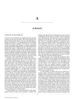
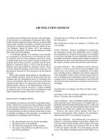
Many discrete probability distributions have been stud-
ied. Perhaps the more familiar of these is the binomial dis-
tribution. In this case there are only two possible events; for
example, heads and tails in coin flipping. The probability
of obtaining x of one of the events in a series of n trials is
described for the binomial distribution by where u is the
probability of obtaining the selected event on a given trial.
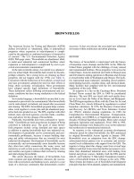
The binomial probability distribution is shown graphically
in Figure 1 for u = 0.5, n = 20.

fx n
n
x
xnx
(;,) ( ) ,uuuϭϪ
Ϫ
⎛
⎝
⎜
⎞
⎠
⎟
1

(1)
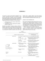
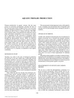
It often happens that we are less concerned with the prob-

ability of an event than in the probability of an event and
all less probable events. In this case, a useful function is the
cumulative distribution which, as its name implies gives for
any value of the random variable, the probability for that
and all lesser values of the random variable. The cumulative
distribution for the binomial distribution is

Fx n fx n
i
x
(;,) (;,).uuϭ
ϭ0
∑

(2)
It is shown graphically in Figure 2 for u = 0.5, n = 20.
An important concept associated with the distribution
is that of the moment. The moments of a distribution are
defined as

m
ki
k
i
i
n
xfxϭ
ϭ
()
1

∑

(3)

NUMBER OF X
5
10 15
20
0
.05
.10
.15
.20
f(X)
FIGURE 1
C019_004_r03.indd 1123C019_004_r03.indd 1123 11/18/2005 1:30:55 PM11/18/2005 1:30:55 PM
© 2006 by Taylor & Francis Group, LLC
1124 STATISTICAL METHODS FOR ENVIRONMENTAL SCIENCE
for the first, second, third, etc. moment, where f ( x
i
) is the
probability function of the variable x. Moments need not be
taken around the mean of the distribution.
However, this is the most important practical case. The
first and second moments of a distribution are especially
important. The mean itself is the first moment and is the
most commonly used measure of central tendency for a dis-
tribution. The second moment about the mean is known as
the variance. Its positive square root, the standard deviation,
is a common measure of dispersion for most distributions.

For the binomial distribution the first moment is given by
µ = n u (4)
and the second moment is given by

suu
2
1ϭϪn ().

(5)

The assumptions underlying the binomial distribution are that
the value of u is constant over trials, and that the trials are
independent; the outcome of one trial is not affected by the
outcome of another trial. Such trials are called Bernoulli trials.
The binomial distribution applies in the case of sampling with
replacement. Where sampling is without replacement, the
hypergeometric distribution is appropriate. A generalization
of the binomial, the multinomial, applies when more than two
outcomes are possible for a single trial.
The Poisson distribution can be regarded as the limit-
ing case of the binomial where n is very large and u is very
small, such that n u is constant. The Poisson distribution is
important in environmental work. Its probability function is
given by

fx
e
x
x
(;)

!
,l
l
l
ϭ
Ϫ

(6)

where l = n u remains constant.
Its first and second moments are
mϭ␭ (7)
s
2
ϭ␭. (8)
The Poisson distribution describes events such as the
probability of cyclones in a given area for given periods of
time, or the distribution of traffic accidents for fixed periods
of time. In general, it is appropriate for infrequent events,
with a fixed but small probability of occurrence in a given
period. Discussions of discrete probability distributions can
be found in Freund among others. For a more extensive dis-
cussion, see Feller.
Continuous Distributions
The distributions mentioned in the previous section are all
discrete distributions; that is, they describe the distribution
of random variables which can be taken on only discrete
values.
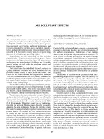
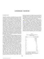
Not all variables of interest take on discrete values; very
commonly, such variables are continuous. The analogous

function to the probability function of a discrete distribution
is the probability density function. The probability density
function for the standard normal distribution is given by

fx e
x
() .
/
ϭ
Ϫ
1
2
2
2
p

(9)
It is shown in Figure 3.
Its first and second moments are
given by

m
p
ϭϭ
Ϫր
Ϫϱ
ϱ
1
2
0

2
2
xe x
x
∫
d

(10)

and

s
p
222
1
2
1
2
ϭϭ
Ϫր
ϱ
ϱ
xe x
x
−
∫
d.

(11)
0

5
10
15
20
NUMBER OF X
F(X)
2.5
7.5
1.0
.5
FIGURE 2
–3 –2 –1 0 1 2 3
X(σ UNITS)
f(X)
0.0
0.1
0.2
0.3
0.4
FIGURE 3
C019_004_r03.indd 1124C019_004_r03.indd 1124 11/18/2005 1:30:56 PM11/18/2005 1:30:56 PM
© 2006 by Taylor & Francis Group, LLC
STATISTICAL METHODS FOR ENVIRONMENTAL SCIENCE 1125
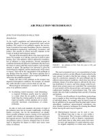
The distribution function for the normal distribution is
given by

Fx e t
t
x
() .ϭ

Ϫր
Ϫϱ
1
2
2
2
p
∫
d

(12)

It is shown in Figure 4.
The normal distribution is of great importance for any
field which uses statistics. For one thing, it applies where the
distribution is assumed to be the result of a very large number
of independent variable, summed together. This is a common
assumption for errors of measurement, and it is often made
for any variables affected by a large number of random fac-
tors, a common situation in the environmental field.
There are also practical considerations involved in the
use of normal statistics. Normal statistics have been the
most extensively developed for continuous random vari-
ables; analyses involving nonnormal assumptions are apt
to be cumbersome. This fact is also a motivating factor in
the search for transformations to reduce variables which are
described by nonnormal distributions to forms to which the
normal distribution can be applied. Caution is advisable,
however. The normal distribution should not be assumed as
a matter of convenience, or by default, in case of ignorance.

The use of statistics assuming normality in the case of vari-
ables which are not normally distributed can result in serious
errors of interpretation. In particular, it will often result in
the finding of apparent significant differences in hypothesis
testing when in fact no true differences exists.
The equation which describes the density function of the
normal distribution is often found to arise in environmental
work in situations other than those explicitly concerned with
the use of statistical tests. This is especially likely to occur in
connection with the description of the relationship between
variables when the value of one or more of the variables may
be affected by a variety of other factors which cannot be
explicitly incorporated into the functional relationship. For
example, the concentration of emissions from a smokestack
under conditions where the vertical distribution has become
uniform is given by Panofsky as

C
Q
VD
e
y
yy
ϭ
Ϫր
2
22
2
ps
s

,

(13)
where y is the distance from the stack, Q is the emission
rate from the stack, D is the height of the inversion layer,
and V is the average wind velocity. The classical diffusion
equation was found to be unsatisfactory to describe this
process because of the large number of factors which can
affect it.
The lognormal distribution is an important non-normal
continuous distribution. It can be arrived at by considering
a theory of elementary errors combined by a multiplicative
process, just as the normal distribution arises out of a theory
of errors combined additively. The probability density func-
tion for the lognormal is given by

fx x
fx
x
ex
nx
()
() .
()
ϭՅ
ϭϾ
ϪϪր
00
1
2

0
12
22
for
for
ps
ms

(14)
The shape of the lognormal distribution depends on the
values of µ and s
2
. Its density function is shown graphically
in Figure 5
for µ = 0, s = 0.5. The positive skew shown is
characteristic of the lognormal distribution.
The lognormal distribution is likely to arise in situa-
tions in which there is a lower limit on the value which
the random variable can assume, but no upper limit. Time
measurements, which may extend from zero to infinity, are
often described by the lognormal distribution. It has been
applied to the distribution of income sizes, to the relative
abundance of different species of animals, and has been
assumed as the underlying distribution for various discrete
counts in biology. As its name implies, it can be normal-
ized by transforming the variable by the use of logarithms.
See Aitchison and Brown (1957) for a further discussion of
the lognormal distribution.
Many other continuous distributions have been studied.
Some of these, such as the uniform distribution, are of minor

–3 –2
–1
012
3
0.0
0.2
0.4
0.6
0.8
1.0
F(X)
X(σ UNITS)
FIGURE 4
0
2
4
6
0.2
0.4
0.6
f(X)
FIGURE 5
C019_004_r03.indd 1125C019_004_r03.indd 1125 11/18/2005 1:30:56 PM11/18/2005 1:30:56 PM
© 2006 by Taylor & Francis Group, LLC
1126 STATISTICAL METHODS FOR ENVIRONMENTAL SCIENCE
importance in environmental work. Others are encountered
occasionally, such as the exponential distribution, which
has been used to compute probabilities in connection with
the expected failure rate of equipment. The distribution of
times between occurrences of events in Poisson processes are

described by the exponential distribution and it is important
in the theory of such stochastic processes (Parzen, 1962).
Further discussion of continuous distributions may be found
in Freund (1962) or most other standard statistical texts.
A special distribution problem often encountered in envi-
ronmental work is concerned with the occurrence of extreme
values of variables described by any one of several distribu-
tions. For example, in forecasting floods in connection with
planning of construction, or droughts in connection with
such problems as stream pollution, concern is with the most
extreme values to be expected. To deal with such problems,
the asymptotic theory of extreme values of a statistical vari-
able has been developed. Special tables have been developed
for estimating the expected extreme values for several dis-
tributions which are unlimited in the range of values which
can be taken on by their extremes. Some information is also
available for distributions with restricted ranges. An interest-
ing application of this theory to prediction of the occurrence
of unusually high tides may be found in Pfafflin (1970) and
the Delta Commission Report (1960) Further discussion
may be found in Gumbel.
HYPOTHESIS TESTING
Sampling Considerations
A basic consideration in the application of statistical pro-
cedures is the selection of the data. In parameter estimation
and hypothesis testing sample data are used to make infer-
ences to some larger population. The data are assumed to
be a random sample from this population. By random we
mean that the sample has been selected in such a way that
the probability of obtaining any particular sample value

is the same as its probability in the sampled population.
When the data are taken care must be used to insure that the
data are a random sample from the population of interest,
and make sure that there must be no biases in the selec-
tive process which would make the samples unrepresenta-
tive. Otherwise, valid inferences cannot be made from the
sample to the sampled population.
The procedures necessary to insure that these conditions
are met will depend in part upon the particular problem being
studied. A basic principle, however, which applies in all
experimental work is that of randomization. Randomization
means that the sample is taken in such a way that any uncon-
trolled variables which might affect the results have an equal
chance of affecting any of the samples. For example, in agri-
cultural studies when plots of land are being selected, the
assignment of different experimental conditions to the plots
of land should be done randomly, by the use of a table of
random numbers or some other randomizing process. Thus,
any differences which arise between the sample values as
a result of differences in soil conditions will have an equal
chance of affecting each of the samples.
Randomization avoids error due to bias, but it does
nothing about uncontrolled variability. Variability can be
reduced by holding constant other parameters which may
affect the experimental results. In a study comparing the
smog-producing effects of natural and artificial light, other
variables, such as temperature, chamber dilution, and so on,
were held constant (Laity, 1971) Note, however, that such
control also restricts generalization of the results to the con-
ditions used in the test.

Special sampling techniques may be used in some cases
to reduce variability. For example, suppose that in an agricul-
tural experiment, plots of land must be chosen from three dif-
ferent fields. These fields may then be incorporated explicitly
into the design of the experiment and used as control vari-
ables. Comparisons of interest would be arranged so that they
can be made within each field, if possible. It should be noted
that the use of control variables is not a departure from ran-
domization. Randomization should still be used in assigning
conditions within levels of a control variable. Randomization
is necessary to prevent bias from variables which are not
explicitly controlled in the design of the experiment.
Considerations of random sampling and the selection
of appropriate control variables to increase precision of the
experiment and insure a more accurate sample selection can
arise in connection with all areas using statistical methods.
They are particularly important in certain environmental
areas, however. In human population studies great care must
be taken in the sampling procedures to insure representative-
ness of the samples. Simple random sampling techniques are
seldom adequate and more complex procedures, have been
developed. For further discussion of this kind of sampling,
see Kish (1965) and Yates (1965). Sampling problems arise
in connection with inferences from cloud seeding experi-
ments which may affect the generality of the results (Bernier,
1967). Since most environmental experiments involve vari-
ables which are affected by a wise variety of other variables,
sampling problems, especially the question of generalization
from experimental results, is a very common problem. The
specific randomization procedures, control variables and

limitations on generalization of results will depend upon the
particular field in question, but any experiment in this area
should be designed with these problems in mind.
Parameter Estimation
A common problem encountered in environmental work is
the estimation of population parameters from sample values.
Examples of such estimation questions are: What is the
“best” estimate of the mean of a population: Within what
range of values can the mean safely be assumed to lie?
In order to answer such questions, we must decide what
is meant by a “best” estimate. Probably the most widely used
method of estimation is that of maximum likelihood, devel-
oped by Fisher (1958). A maximum likelihood estimate is one
which selects that parameter value for a distribution describing
C019_004_r03.indd 1126C019_004_r03.indd 1126 11/18/2005 1:30:56 PM11/18/2005 1:30:56 PM
© 2006 by Taylor & Francis Group, LLC
STATISTICAL METHODS FOR ENVIRONMENTAL SCIENCE 1127
a population which maximizes the probability of obtaining the
observed set of sample values, assuming random sampling. It
has the advantages of yielding estimates which fully utilize the
information in the sample, if such estimates exist, and which
are less variable under certain conditions for large samples
than other estimates.
The method consists of taking the equation for the prob-
ability, or probability density function, finding its maximum
value, either directly or by maximizing the natural loga-
rithm of the function, which has a maximum for the same
parameter values, and solving for these parameter values.
The sample mean,

m
^
= (⌺
n
i=1
x
i
)/Nu , is a maximum likelihood
estimate of the true mean of the distribution for a number of
distributions. The variance,

s
^
2
, calculated from the sample
by

s
^
2
= (⌺
n
i=1
(x
i
-m
^
)
2
, is a maximum likelihood estimate of the

population s
2
for the normal distribution.
Note that such estimates may not be the best in some
other sense. In particular, they may not be unbiased. An
unbiased estimate is one whose value will, on the average,
equal that of the parameter for which it is an estimate, for
repeated sampling. In other words, the expected value of
an unbiased estimate is equal to the value of the parameter
being estimated. The variance is, in fact, biased. To obtain an
unbiased estimate of the population variance it is necessary
to multiply s
2
by n /( n Ϫ 1), to yield s
2
, the sample variance,
and s, (ϩ͌s
2
)

the sample standard deviation.
There are other situations in which the maximum like-
lihood estimate may not be “best” for the purposes of the
investigator. If a distribution is badly skewed, use of the
mean as a measure of central tendency may be quite mis-
leading. It is common in this case to use the median, which
may be defined as the value of the variable which divides the
distribution into two equal parts. Income statistics, which are
strongly skewed positively, commonly use the median rather
than the mean for this reason.

If a distribution is very irregular, any measure of central
tendency which attempts to base itself on the entire range of
scores may be misleading. In this case, it may be more useful
to examine the maximum points of f ( x ); these are known as
modes. A distribution may have 1, 2 or more modes; it will
then be referred to as unimodal, bimodal, or multimodal,
respectively.
Other measures of dispersion may be used besides the
standard deviation. The probable error, p.e., has often been
used in engineering practice. It is a number such that

fxdx
pe
pe
()


ϭ
Ϫ
ϩ
05
m
m
∫

(15)

The p.e. is seldom used today, having been largely replaced
by s
2

.
The interquartile range may sometimes be used for a set
of observations whose true distribution is unknown. It con-
sists of the limits of the range of values which include the
middle half of sample values. The interquartile range is less
sensitive than the standard deviation to the presence of a few
very deviant data values.
The sample mean and standard deviation may be used to
describe the most likely true value of these parameters, and
to place confidence limits on that value. The standard error
of the mean is given by

s/͌n ( n = sample-size). The stan-
dard error of the mean can be used to make a statement about
the probability that a range of values will include the true
mean. For example, assuming normality, the range of values
defined by the observed mean 1.96s/͌n will be expected to
include the value of the true mean in 95% of all samples.
A more general approach to estimation problems can be
found in Bayseian decision theory (Pratt et al. , 1965). It is pos-
sible to appeal to decision theory to work out specific answers
to the “best estimate” problem for a variety of decision cri-
teria in specific situations. This approach is well described
in Weiss (1961). Although the method is not often applied
in routine statistical applications, it has received attention in
systems analysis problems and has been applied to such envi-
ronmentally relevant problems as resource allocation.
Frequency Data
The analysis of frequency data is a problem which often
arises in environmental work. Frequency data for a hypo-

thetical experiment in genetics are shown in Table 1. In this
example, the expected frequencies are assumed to be known
independently of the observed frequencies. The chi-square
statistic, x
2
, is defined as

x
2
2
2
ϭ
Ϫ()EO
E
∑

(16)

where E is the expected frequency and O is the observed
frequency. It can be applied to frequency tables, such as that
shown in Table 1. Note that an important assumption of the
chi-square test is that the observations be independent. The
same samples or individuals must not appear in more than
one cell.
In the example given above, the expected frequencies
were assumed to be known. In practice this is very often not
the case; the experimenter will have several sets

TABLE 1
Hypothetical data on the frequency of plants producing red, pink and white

flowers in the first generation of an experiment in which red and white
parent plants were crossed, assuming single gene inheritance, neither gene
dominant of observed frequencies, and will wish to determine whether
or not they represent samples from one population, but will not know the
expected frequency for samples from that population.
Flower color
Red Pink White
Number of
plants
expected 25 50 25
observed 28 48 24
C019_004_r03.indd 1127C019_004_r03.indd 1127 11/18/2005 1:30:56 PM11/18/2005 1:30:56 PM
© 2006 by Taylor & Francis Group, LLC
1128 STATISTICAL METHODS FOR ENVIRONMENTAL SCIENCE
In situations where a two-way categorization of the data
exists, the expected values may be estimated from the mar-
ginals. For example, the formula for chi-square for the four-
fold contingency table shown below is
Classification II
Classification I A B
CD

x
2
2
2
ϭ
ԽϪԽϪNADBC
N
ABCD

⎛
⎝
⎜
⎞
⎠
⎟
⋅⋅⋅
.

(17)

Observe that instead of having independent expected values,
we are now estimating these parameters from the marginal
distributions of the data. The result is a loss in the degrees
of freedom for the estimate. A chi-square with four indepen-
dently obtained expected values would have four degrees of
freedom; the fourfold table above has only one. The con-
cept of degrees of freedom is a very general one in statistical
analysis. It is related to the number of observations which can
vary independently of each other. When expected values for
chi-square are computed from the marginals, not all of the
O Ϫ E differences in a row or column are independent, for their
discrepancies must sum to zero. Calculation of means from
sample data imposes a similar restriction; since the deviations
from the mean must sum to zero, not all of the observations in
the sample can be regarded as freely varying. It is important to
have the correct number of degrees of freedom for an estimate
in order to determine the proper level of significance; many
statistical tables require this information explicitly, and it is
implicit in any comparison. Calculation of the proper degrees

of freedom for a comparison can become complicated in spe-
cific cases, especially that of analysis of variance. The basic
principle to remember, however, is that any linear independent
constraints placed on the data will reduce the degrees of free-
dom. Tables for value of the x
2
distribution for various degrees
of freedom are readily available. For a further discussion of
the use of chi-square, see Snedecor.
Difference between Two Samples
Another common situation arises when two samples are
taken, and the experimenter wishes to know whether or not
they are samples from populations with the same parameter
values. If the populations can be presumed to be normal,
then the significance of the differences of the two means can
be tested by

t
s
N
s
N
ϭ
ϩ
ˆˆ
mm
12
1
2
1

2
2
2
−

(18)

where

m
^
1
and

m
^
2
are the sample means, s
2
1
and

s
2
1
are the
sample variances, N
1
and N
2

are the sample sizes. and the
population variances are assumed to be equal. This is the
t -test, for two samples. The t -test can also be used to test the
significance of the difference between one sample mean and
a theoretical value. Tables for the significance of the t -test
may be found in most statistical texts.
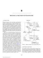
The theory underlying the t -test is that the measures of
dispersion estimated from the observations within a sample
provide estimates of the expected variability. If the means are
close together, relative to that variability, then it is unlikely
that the populations differ in their true values. However, if
the means vary widely, then it is unlikely that the samples
come from distributions with the same underlying distribu-
tions. This situation is diagrammed in Figure 6.
The t -test
permits an exact statement of how unlikely the null hypoth-
esis (assumption of no difference) is. If it is sufficiently
unlikely, it can be rejected. It is common to assume the null
hypothesis unless it can be rejected in at least 95% of the
cases, though more stringent criteria (99% or more) may be
adopted if more certainty is needed.
The more stringent the criterion, of course, the more likely
it is that the null hypothesis will be accepted when, in fact, it
is false. The probability of falsely rejecting the null hypoth-
esis is known as a type I error. Accepting the null hypothesis
when it should be rejected is known as a type II error. For a
given type I error, the probability of correctly rejecting the
null hypothesis for a given true difference is known as the
power of the test for detecting the difference. The function of
these probabilities for various true differences in the param-

eter under test is known as the power function of the test.
Statistical tests differ in their power and power functions are
useful in the comparison of different tests.
Note that type I and type II errors are necessarily related;
for an experiment of a given level of precision, decreasing
the probability of a type I error raises the probability of a
type II error, and vice versa. Thus, increasing the stringency
of one’s criterion does not decrease the overall probability
of an erroneous conclusion; it merely changes the type of
error which is most likely to be made. To decrease the over-
all error, the experiment must be made more precise, either
by increasing the number of observations, or by reducing the
error in the individual observations.
Many other tests of mean difference exist besides
the t-test. The appropriate choice of a test will depend on
the assumptions made about the distribution underlying the
observations. In theory, the t-test applies only for variables
which are continuous, range from ± infinity in value, and
X (σ UNITS)
f(X)
m
1
m
2
m
3
FIGURE 6
C019_004_r03.indd 1128C019_004_r03.indd 1128 11/18/2005 1:30:56 PM11/18/2005 1:30:56 PM
© 2006 by Taylor & Francis Group, LLC
STATISTICAL METHODS FOR ENVIRONMENTAL SCIENCE 1129

are normally distributed with equal variance assumed for the
underlying population. In practice, it is often applied to vari-
ables of a more restricted range, and in some cases where the
observed values of a variable are inherently discontinuous.
However, when the assumptions of the test are violated, or
distribution information is unavailable, it may be safer to use
nonparametric tests, which do not depend on assumptions
about the shape of the underlying distribution. While non-
parametric tests are less powerful than parametric tests such
as the t-test, when the assumptions of the parametric tests
are met, and therefore will be less likely to reject the null
hypothesis, in practice they yield results close to the t-test
unless the assumptions of the t-test are seriously violated.
Nonparametric tests have been used in meteorological stud-
ies because of nonnormality in the distribution of rainfall
samples. (Decker and Schickedanz, 1967). For further dis-
cussions of hypothesis testing, see Hoel (1962) and Lehmann
(1959). Discussions of nonparametric tests may be found in
Pierce (1970) and Siegel (1956).
Analysis of Variance (ANOVA)
The t-test applies to the comparison of two means. The con-
cepts underlying the t-test may be generalized to the testing of
more than two means. The result is known as the analysis of
variance. Suppose that one has several samples. A number
of variances may be estimated. The variance of each sample
can be computed around the mean for the sample. The vari-
ance of the sample means around the grand mean of all the
scores gives another variance. Finally, one can ignore the
grouping of the data and complete the variance for all scores
around the grand mean. It can be shown that this “total” vari-

ance can be regarded as made up of two independent parts,
the variance of the scores about their sample means, and the
variance of these means about the grand mean. If all these
samples are indeed from the same population, then estimates
of the population variance obtained from within the individ-
ual groups will be approximately the same as that estimated
from the variance of sample means around the grand mean.
If, however, they come from populations which are normally
distributed and have the same standard deviations, but dif-
ferent means, then the variance estimated from the sample
means will exceed the variance are estimated from the within
sample estimates.
The formal test of the hypothesis is known as the F-test.
It is made by forming the F-ratio.

F =
MSE
MSE
(1)
(2)

(19)
Mean square estimates (MSE) are obtained from variance
estimates by division by the appropriate degrees of free-
dom. The mean square estimate in the numerator is that for
the hypothesis to be tested. The mean square estimate in
the denominator is the error estimate; it derives from some
source which is presumed to be affected by all sources of
variance which affect the numerator, except those arising
from the hypothesis under test. The two estimates must also

be independent of each other. In the example above, the
within group MSE is used as the error estimate; however,
this is often not the case for more complex experimental
designs. The appropriate error estimate must be determined
from examination of the particular experimental design, and
from considerations about the nature of the independent
variables whose effect is being tested; independent variables
whose values are fixed may require different error estimates
than in the case of independent variables whose values are
to be regarded as samples from a larger set. Determination
of degrees of freedom for analysis of variance goes beyond
the scope of this paper, but the basic principle is the same
as previously discussed; each parameter estimated from the
data (usually means, for (ANOVA) in computing an estima-
tor will reduce the degrees of freedom for that estimate.
The linear model for such an experiment is given by
X
ij
= µ + G
i
+ e
ij,
(20)
Where X
ij
is a particular observation, µ is the mean, G
i
is
the effect the Gth experimental condition and e
ij

is the
error uniquely associated with that observation. The e
ij
are
assumed to be independent random samples from normal
distributions with zero mean and the same variances. The
analysis of variance thus tests whether various components
making up a score are significantly different from zero.
More complicated components may be presumed. For
example, in the case of a two-way table, the assumed model
might be
X
ijk
= µ + R
i
+ C
j
+ R
cij
+ e
ijk
(21)
In addition to having another condition, or main effect, there
is a term RC
ij
which is associated with that particular combi-
nation of levels of the main effects. Such effects are known
as interaction effects.
Basic assumptions of the analysis of variance are nor-
mality and homogeneity of variance. The F-test however,

has been shown to be relatively “robust” as far as deviations
from the strict assumption of normality go. Violations of the
assumption of homogeneity of variance may be more seri-
ous. Tests have been developed which can be applied where
violations of this assumption are suspected. See Scheffé
(1959; ch.10) for further discussion of this problem.
Innumerable variations on the basic models are possible.
For a more detailed discussion, see Cochran and Cox (1957) or
Scheffé (1959). It should be noted, especially, that a significant
F-ratio does not assure that all the conditions which entered
into the comparison differ significantly from each other. To
determine which mean differences are significantly differ-
ent, additional tests must be made. The problem of multiple
comparisons among several means has been approached in
three main ways; Scheffé’s method for post-hoc comparisons;
Tukey’s gap test; and Duncan’s multiple range test. For further
discussion of such testing, see Kirk (1968).
Computational formulas for ANOVA can be found in
standard texts covering this topic. However, hand calculation
C019_004_r03.indd 1129C019_004_r03.indd 1129 11/18/2005 1:30:57 PM11/18/2005 1:30:57 PM
© 2006 by Taylor & Francis Group, LLC
1130 STATISTICAL METHODS FOR ENVIRONMENTAL SCIENCE
becomes cumbersome for problems of any complexity, and
a number of computer programs are available for analyzing
various designs. The Biomedical Statistical Programs (Ed. by
Dixon 1967) are frequently used for this purpose. A method
recently developed by Fowlkes (1969) permits a particularly
simple specification of the design problem and has the flex-
ibility to handle a wide variety of experimental designs.
SPECIAL ESTIMATION PROBLEMS

The estimation problems we have considered so far have
involved single experiments, or sets of data. In environmen-
tal work, the problem of arriving at an estimate by combin-
ing the results of a series of tests often arises. Consider, for
example, the problem of estimating the coliform bacteria
population size in a specimen of water from a series of dilu-
tion tests. Samples from the water specimen are diluted by
known amounts. At some point, the dilution becomes so
great that the lactose broth brilliant green bile test for the
presence of coliform bacteria becomes negative (Fair and
Geyer, 1954). From the amount of dilution necessary to
obtain a negative test, plus the assumption that one organism
is enough to yield a positive response, it is possible to esti-
mate the original population size in the water specimen.
In making such an estimate, it is unsatisfactory simply
to use the first negative test to estimate the population size.
Since the diluted samples may differ from one another, it is
possible to get a negative test followed by one or more posi-
tive tests. It is desirable, rather, to estimate the population
from the entire series of tests. This can be done by setting
up a combined hypothesis based on the joint probabilities of
all the obtained results, and using likelihood estimation pro-
cedures to arrive at the most likely value for the population
parameter, which is known as the Most Probable Number
(MPN) (Fair and Geyer, 1954). Tables have been prepared
for estimating the MPN for such tests on this principle, and
similar procedures can be used to arrive at the results of a set
of tests in other situations.
Sequential testing is a problem that sometimes arises in
environmental work. So far, we have assumed that a con-

stant amount of data is available. However, very often, the
experimenter is making a series of tests, and wishes to know
whether he has enough data to make a decision at a given
level of reliability, or whether he should consider taking
additional data. Such estimation problems are common in
quality control, for example, and may arise in connection
with monitoring the effluent from various industrial pro-
cesses. Statistical procedures have been developed to deal
with such questions. They are discussed in Wald.
CORRELATION AND RELATED TOPICS
So far we have discussed situations involving a single vari-
able. However, it is common to have more than one type
of measure available on the experimental units. The sim-
plest case arises where values for two variables have been
obtained, and the experimenter wishes to know how these
variables relate to one another.
Curve Fitting
One problem which frequently arises in environmental work
is the fitting of various functions to bivariate data. The sim-
plest situation involves fitting a linear function to the data
when all of the variability is assumed to be in the Y variable.
The most commonly used criterion for fitting such a function
is the minimization of the squared deviations from the line,
referred to as the least squares criterion. The application of
this criterion yields the following simultaneous equations:

YnA X
i
i
n

i
i
n
ϭϩ
ϭϭ11
∑∑

(22)

and

XY A X B X
ii
i
n
i
i
n
i
i
n
ϭϩ
ϭϭϭ11
2
1
∑∑∑
.

(22)
These equations can be solved for A and B, the intercept and

slope of the best fit line. More complicated functions may
also be fitted, using the least squares criterion, and it may be
generalized to the case of more than two variables. Discussion
of these procedures may be found in Daniel and Wood.
Correlation and Regression
Another method of analysis often applied to such data is
that of correlation. Suppose that our two variables are both
normally distributed. In addition to investigating their indi-
vidual distributions, we may wish to consider their joint
occurrence. In this situation, we may choose to compute the
Pearson product moment correlation between the two vari-
ables, which is given by

r
xy
xy
ii
xy
ϭ
cov( )
ss

(23)
where cov( x
i
y
i
) the covariance of x and y, is defined as

()()

.
xy
n
ixiy
i
n
ϪϪ
ϭ
mm
1
∑

(24)

It is the most common measure of correlation. The square
of r gives the proportion of the variance associated with one
of the variables which can be predicted from knowledge of
the other variables. This correlation coefficient is appropri-
ate whenever the assumption of a normal distribution can be
made for both variables.
C019_004_r03.indd 1130C019_004_r03.indd 1130 11/18/2005 1:30:57 PM11/18/2005 1:30:57 PM
© 2006 by Taylor & Francis Group, LLC
STATISTICAL METHODS FOR ENVIRONMENTAL SCIENCE 1131
Another way of looking at correlation is by consider-
ing the regression of one variable on another. Figure 7
shows the relation between two variables, for two sets of
bivariate data, one with a 0.0 correlation, the other with a
correlation of 0.75. Obviously, estimates of type value of one
variable based on values of the other are better in the case of
the higher correlation. The formula for the regression of y on

x is given by

yrx
y
y
xy x
x
Ϫ
ϭ
Ϫ
ˆ
ˆ
(
ˆ
)
(
ˆ
)
.
m
s
m
s

(25)

A similar equation exists for the regression of x on y.
A number of other correlation measures are available.
For ranked data, the Spearman correlation coefficient, or
Kendall’s tau, are often used. Measures of correlation appro-

priate for frequency data also exist. See Siegel.
MULTIVARIATE ANALYSIS
Measurements may be available on more than two variables
for each experiment. The environmental field is one which
offers great potential for multivariate measurement. In areas of
environmental concern such as water quality, population stud-
ies, or the study of the effects of pollutants on organisms, to
name only a few, there are often several variables which are of
interest. The prediction of phenomena of environmental inter-
est, or such as rainfall, or floods, typically involves the consid-
eration of many variables. This section will be concerned with
some problems in the analysis of multivariate data.
Multivariate Distributions
In considering multivariate distributions, it is useful to define
the n -dimensional random variable X as the vector

′
XXXX
n
ϭ[, , ].
12
,Κ

(26)
The elements of this vector will be assumed to be con-
tinuous unidimensional random variables, with density
functions

f
1

(x
1
),Ff
2
(x
2
)K,f
n
(x
n
) and distribution functions

F
1
(x
1
),F
2
(x
2
)K,F
n
(x
n
) Such a vector also has a joint distribu-
tion function.

Fx x x PX x X x
nnn
(, ,, ) ( ,, )

12 1 1
ΚΚ= ՅՅ

(27)

where P refers to the probability of all the stated conditions
occurring simultaneously.
The concepts considered previously in regard to univari-
ate distribution may be generalized to multivariate distri-
butions. Thus, the expected value of the random vector, X,
analogous to the mean of the univariate distribution, is

EX EX EX EX
n
( ) [ ( ), ( ), ( )],
′
ϭ
12
K

(28)

where the E ( X
i
) are the expected values, or means, for the
univariate distributions.
Generalization of the concept of variance is more com-
plicated. Let us start by considering the covariance between
two variables,

s
ij i i j j
EX EX X EXϭϪ Ϫ[ ( )][ ( )].
(29)
The covariances between each of the elements of the vector
X can be computed; the covariances of the i th and j th ele-
ments will be designed as

s
ij
If i = j the covariance is the
r = 0.0
r = 0.75
X
X
FIGURE 7
C019_004_r03.indd 1131C019_004_r03.indd 1131 11/18/2005 1:30:57 PM11/18/2005 1:30:57 PM
© 2006 by Taylor & Francis Group, LLC
1132 STATISTICAL METHODS FOR ENVIRONMENTAL SCIENCE
variance of X
i
, and will be designed as

s
ij

The generalization
of the concept of variance to a multidimensional variable
then becomes the matrix of variances and covariances. This
matrix will be called the covariance matrix. The covariance

matrix for the population is given as

∑
⎡
⎣
⎢
⎢
⎢
⎢
⎢
⎤
⎦
⎥
⎥
⎥
⎥
⎥
ϭ
sss
sss
sss
11 12 1
21 22 2
122
Κ
Κ
ΚΚΚΚΚ
…
n
n

nn nn
.

(30)
A second useful matrix is the matrix of correlations

rr
rr
rr
n
n
nnn
11 1
21 2
1
⌳
⌳
⌳⌳⌳
…
⎡
⎣
⎢
⎢
⎢
⎢
⎢
⎤
⎦
⎥
⎥

⎥
⎥
⎥

(31)

If the assumption is made that each of the individual vari-
ables is described by a normal distribution, then the distri-
bution of X may be described by the multivariate normal
distribution. This assumption will be made in subsequent
discussion, except where noted to the contrary.
Tests on Means
Suppose that measures have been obtained on several vari-
ables for a sample, and it is desired to determine whether that
sample came from some known population. Or there may be
two samples; for example, suppose data have been gathered
on physiological effects of two concentrations of SO
2
for
several measures of physiological functioning and the inves-
tigator wishes to know if they should be regarded as samples
from the same population. In such situations, instead of using
t -tests to determine the significance of each individual differ-
ence separately, it would be desirable to be able to perform
one test, analogous to the t -test, on the vectors of the means.
A test, known as Hotelling’s T

2
test, has been developed
for this purpose. The test does not require that the popula-

tion covariance matrix be known. It does, however, require
that samples to be compared come from populations with
the same covariance matrix, an assumption analogous to the
constant variance requirement of the t -test.
To understand the nature of T

2
in the single sample case,
consider a single random variable made up of any linear
combination of the n variables in the vector X (all of the
variables must enter into the combination, that is, none of the
coefficients may be zero). This variable will have a normal
distribution, since it is a sum of normal variables, and it can
be compared with a linear combination of elements from
the vector for the population with the same coefficients, by
means of a t -test. We then adopt the decision rule that the null
hypothesis will be accepted only if it is true for all possible
linear combinations of the variables. This is equivalent to
saying that it is true for the largest value of t as a function of
the linear combinations. By maximizing t
2
as a function of
the linear combinations, it is possible to derive T

2
. Similar
arguments can be used to derive T

2
for two samples.

A related function of the mean is known as the linear
discriminant function. The linear discriminant function is
defined as the linear compound which generates the largest
T

2
value. The coefficients used in this compound provide
the best weighting of the variables of a multivariate obser-
vation for the purpose of deciding which population gave
rise to an observation. A limitation on the use of the linear
discriminant function, often ignored in practice, is that it
requires that the parameters of the population be known, or
at least be estimated from large samples. This statistic has
been used in analysis of data from monitoring stations to
determine whether pollution concentrations exceed certain
criterion values.
Other statistical procedures employing mean vectors are
useful in certain circumstances. See Morrison for a further
discussion of this question.
Multivariate Analysis of Variance (MANOVA)
Just as the concepts underlying the t -test could be general-
ized to the comparison of more than two means, the concepts
underlying the comparison of two mean vectors can be gen-
eralized to the comparison of several vectors of means.
The nature of this generalization can be understood in
terms of the linear model, considered previously in connec-
tion with analysis of variance. In the multivariate situation,
however, instead of having a single observation which is
hypothesized to be made up of several components com-
bined additively, the observations are replaced by vectors of

observations, and the components by vectors of components.
The motivation behind this generalization is similar to that
for Hotelling’s T
2
test: it permits a test of the null hypothesis
for all of the variables considered simultaneously.
Unlike the case of Hotelling’s T
2
, however, various
methods of test construction do not converge on one test sta-
tistic, comparable to the F test for analysis of variance. At
least three test statistics have been developed for MANOVA,
and the powers of the various tests in relation to each other
are very incompletely known.
Other problems associated with MANOVA are similar in
principle to those associated with ANOVA, though computa-
tionally they are more complex. For example, the problem of
multiple comparison of means has its analogous problem in
MANOVA, that of determining which combinations of mean
vectors are responsible for significant test statistics. The
number and type of possible linear models can also ramify
considerably, just as in the case of ANOVA. For further dis-
cussion of MANOVA, see Morrison (1967) or Seal.
Extensions of Correlation Analysis
In a number of situations, where multivariate measurements
are taken, the concern of the investigator centers on the
C019_004_r03.indd 1132C019_004_r03.indd 1132 11/18/2005 1:30:57 PM11/18/2005 1:30:57 PM
© 2006 by Taylor & Francis Group, LLC
STATISTICAL METHODS FOR ENVIRONMENTAL SCIENCE 1133
prediction of one of the variables. When rainfall measure-

ments are taken in conjunction with a number of other vari-
ables, such as temperature, pressure, and so on, for example,
the purpose is usually to predict the rainfall as a function of
the other variables. Thus, it is possible to view one variable
as the dependent variable for a prior reasons, even though
the data do not require such a view.
In these situations, the investigator very often has one of
two aims. He may wish to predict one of the variables from
all of the other variables. Or he may wish to consider one
variable as a function of another variable with the effect of
all the other variables partialled out. The first situation calls
for the use of multiple correlation. In the second, the appro-
priate statistic is the partial correlation coefficient.
Multiple correlation coefficients are used in an effort to
improve prediction by combining a number of variables to
predict the variable of interest. The formula for three vari-
ables is

r
rr rrr
r
123
12
2
13
2
12 13 23
23
2
2

1
.
.ϭ
ϩϪ
Ϫ

(32)

Generalizations are available for larger numbers of variables.
If the variables are relatively independent of each other, mul-
tiple correlation may improve prediction. However, it should
be obvious that this process reaches an upper limit since
additional variables, if they are to be of any value, must show
a reasonable correlation with the variable of interest, and the
total amount of variance to be predicted is fixed. Each addi-
tional variable can therefore only have a limited effect.
Partial correlation is used to partial out the effect of one
of more variables on the correlation between two other vari-
ables. For example, suppose it is desired to study the relation-
ship between body weight and running speed, independent
of the effect of height. Since height and weight are corre-
lated, simply doing a standard correlation between running
speed and weight will not solve the problem. However, com-
puting a partial correlation, with the contribution of height
partialled out, will do so. The partial correlation formula for
three variables is

r
rrr
rr

12 3
12 13 23
13
2
23
2
11
.
,ϭ
Ϫ
ϪϪ

(33)
where r
12.3
gives the correlation of variables 1 and 2, with
the contribution of variable 3 held constant. This formula
may also be extended to partial out the effect of additional
variables.
Let us return for a moment to a consideration of the pop-
ulation correlation matrix, p. It may be that the investigator
has same a priori reason for believing that certain relation-
ships exist among the correlations in this matrix. Suppose,
for example there is a reason to believe that several variables
are heavily dependent on wind velocity and that another set
of variables are dependent on temperature. Such a pattern of
underlying relations would result in systematic patterns of
high and low correlations in the population matrix, which
should be reflected in the observed correlation matrix. If the
obtained correlation matrix is partitioned into sets in accor-

dance with the a priori hypothesis, test for the independence
of the sets will indicate whether or not the hypothesis should
be rejected. Procedures have been developed to deal with
this situation, and also to obtain coefficients reflecting the
correlation between sets of correlations. The latter procedure
is known as canonical correlation. Further information about
these procedures may be found in Morrison.
Other Analyses of Covariance and Correlation
Matrices
In the analyses discussed so far, there have been a priori
considerations guiding the direction of the analysis. The sit-
uation may arise, however, in which the investigator wishes
to study the patterns in an obtained correlation or covariance
matrix without any appeal to a priori considerations. Let us
suppose, for example, that a large number of measurements
relevant to weather prediction have been taken, and the
investigator wishes to look for patterns among the variables.
Or suppose that a large number of demographic variables
have been measured on a human population. Again, it is rea-
sonable to ask if certain of these variables show a tendency
to be more closely related than others, in the absence of any
knowledge about their actual relations. Such analyses may
be useful in situations where large numbers of variables are
known to be related to a single problem, but the relationships
among the variables are not well understood. An investiga-
tion of the correlation patterns may reveal consistencies in
the data which will serve as clues to the underlying process.
The classic case for the application of such techniques
has been the study of the human intellect. In this case, cor-
relations among performances on a very large number of

tasks have been obtained and analyzed, and many theories
about the underlying skills necessary for intellectual func-
tion have been derived from such studies. The usefulness of
the techniques are by no means limited to psychology, how-
ever. Increasingly, they are being applied in other fields, as
diverse as biology (Fisher and Yates, 1964) and archaeology
(Chenhall, 1968). Principal component analysis, a closely
related technique, has been used in hydrology.
One of the more extensively developed techniques for the
analysis of correlation matrices is that of factor analysis. To
introduce the concepts underlying factor analysis, imagine a
correlation matrix in which the first x variables and the last
n Ϫ x variables are all highly correlated with each other,
but the correlation between any of the first x and any of the
second n Ϫ x variables is very low. One might suspect that
there is some underlying factor which influences the first set
of variables, and another which influences the second set of
variables, and that these two factors are relatively indepen-
dent statistically, since the variables which they influence
are not highly correlated. The conceptual simplification is
obvious; instead of worrying about the relationships among
n variables as reflected in their n ( n Ϫ 1)/2 correlations, the
C019_004_r03.indd 1133C019_004_r03.indd 1133 11/18/2005 1:30:57 PM11/18/2005 1:30:57 PM
© 2006 by Taylor & Francis Group, LLC
1134 STATISTICAL METHODS FOR ENVIRONMENTAL SCIENCE
investigator can attempt to identify and measure the factors
directly.
Factor analysis uses techniques from matrix algebra to
accomplish mathematically the process we have outlined
intuitively above. It attempts to determine the number of

factors, and also the extent to which each of these factors
influences the measured variables. Since unique solutions to
this problem do not exist, the technique has been the subject
of considerable debate, especially on the question of how
to determine the best set of factors. Nevertheless, it can be
useful in any situation where the relationships among a large
set of variables is not well understood.
ADDITIONAL PROCEDURES
Multidimensional Scaling and Clustering
There are a group of techniques whose use is motivated by
considerations similar to those underlying the analysis of
correlation matrices, but which are applied directly to matri-
ces of the distances, or similarities, between various stimuli.
Suppose, for example, that people have been asked to judge
the similarity of various countries. These judgments may
be scaled by multidimensional techniques to discover how
many dimensions underlie the judgments. Do people make
such judgments along a single dimension? Or are several
dimensions involved? An interesting example of this sort
was recently analyzed by Wish (1972). Sophisticated tech-
niques have been worked out for such procedures.
Multidimensional scaling has been most extensively
used in psychology, where the structure underlying simi-
larity or distance measurements may not be at all obvious
without such procedures. Some of these applications are of
potential importance in the environmental field, especially
in areas such as urban planning, where decisions must take
into account human reactions. They are not limited to such
situations however, and some intriguing applications have
been made in other fields.

A technique related in some ways to multidimensional
analysis is that of cluster analysis. Clustering techniques
can be applied to the same sort of data as multidimensional
scaling procedures. However, the aim is somewhat differ-
ent. Instead of looking for dimensions assumed to underlie
the data, clustering techniques try to define related clusters
of stimuli. Larger clusters may then be identified, until a
hierarchical structure is defined. If the data are sufficiently
structured, a “Tree” may be derived.
A wide variety of clustering techniques have been
explored, and interest seems on the increase (Johnson,
1967). The procedures used depend upon the principles
used to define the clusters. Clustering techniques have been
applied in a number of different fields. Biologists have used
them to study the relationships among various animals; for
example, a kind of numerical taxonomy.
The requirements which the data must meet for multi-
dimensional scaling and clustering procedures to apply are
usually somewhat less stringent than in the case of the mul-
tivariate procedures discussed previously. Multidimensional
scaling in psychology is often done on data for which an
interval scale of measurement cannot be assumed. Distance
measures for clustering may be obtained from the clustering
judgments of a number of individuals which lack an ordinal
scale. This relative freedom is also useful in many applica-
tions where the order of items is known, but the equivalence
of the distances between items measured at different points
is questionable.
Stochastic Processes
A stochastic or random process is any process which includes

a random element in its description. The term stochastic
process is frequently also used to describe the mathemati-
cal description of any actual stochastic process. Stochastic
models have been developed in a number of areas of envi-
ronmental concern.
Many stochastic processes involve space or time as a
primary variable. Bartlett (1960) in his discussion of eco-
logical frequency distributions begins with the application of
the Poisson distribution to animal populations whose density
is assumed to be homogeneous over space, and then goes
on to develop the consequences of assuming heterogeneous
distributions, which are shown to lead to other distributions,
such as the negative binomial. The Sutton equation for the
diffusion of gases applied to stack effluents, a simplification
of which was given earlier for a single dimension (Strom,
1968) is another example of a situation in which statistical
considerations about the physical process lead to a spatial
model, in this case, one involving two dimensions.
Time is an important variable in many stochastic models.
A number of techniques have been developed for the analy-
sis of time series. Many of the concepts we have already con-
sidered, such as the mean and variance, can be generalized to
time series. The autocorrelation function, which consists of
the correlation of a function with itself for various time lags,
is often applied to time series data. This function is useful in
revealing periodicities in the data, which show up as peaks in
the function. Various modifications of this concept have been
developed to deal with data which are distributed in discrete
steps over time. Time series data, especially discrete time series
data, often arise in such areas as hydrology, and the study of air

pollution, where sampling is done over time. Such sampling is
often combined with spatial sampling, as when meterological
measurements are made at a number of stations.
An important consideration in connection with time
series is whether the series is stationary or non-stationary.
Stationarity of a time series implies that the behavior of the
random variables involved does not depend on the time at
which observation of the series is begun. The assumption of
stationarity simplifies the statistical treatment of time series.
Unfortunately, it is often difficult to justify for environmen-
tal measurements, especially those taken over long time
periods. Examination of time series for evidence of non-sta-
tionarity can be a useful procedure, however; for example,
it may be useful in determining whether long term climatic
changes are occurring (Quick, 1992). For further discussion
of time series analysis, see Anderson.
C019_004_r03.indd 1134C019_004_r03.indd 1134 11/18/2005 1:30:57 PM11/18/2005 1:30:57 PM
© 2006 by Taylor & Francis Group, LLC
STATISTICAL METHODS FOR ENVIRONMENTAL SCIENCE 1135
Stochastic models of environmental interest are often
multivariate. Mathematical models applied to air pollu-
tion may deal with the concentrations of a number of pol-
lutants, as well as such variables as temperature, pressure,
precipitation, and wind direction. Special problems arise in
the evaluation of such models because of the large numbers
of variables involved, the large amounts of data which must
be processed for each variable, and the fact that the distri-
butions of the variables are often nonnormal, or not well
known. Instead of using analytic methods to obtain solu-
tions, it may be necessary to seek approximate solutions; for

example, by extensive tabulation of data for selected sets of
conditions, as has been one in connection with models for
urban air pollution.
The development of computer technology to deal with
the very large amounts of data processing often required has
made such approaches feasible today. Nevertheless, caution
with regard to many stochastic models should be observed.
It is common to find articles describing such models which
state that a number of simplifying assumptions were neces-
sary in order to arrive at a model for which computation
was feasible, and which then go on to add that even with
these assumptions the computational limits of available
facilities were nearly exceeded, a combination which raises
the possibility that excessive simplification may have been
introduced. In these circumstances, less ambitious treat-
ment of the data might prove more satisfactory. Despite
these comments, however, it is clear that the environmental
field presents many problems to which the techniques of
stochastic modelling can be usefully applied.
ADDITIONAL CONSIDERATIONS
The methods outlined in the previous sections represent a
brief introduction to the statistics used in environmental
studies. It appears that the importance of some of these
statistical methods, particularly analysis of variance, multi-
variate procedures and the use of stochastic modelling will
increase. The impact of computer techniques has been great
on statistical computations in environmental fields. Large
amounts of data may be collected and processed by com-
puter methods.
ACKNOWLEDGMENTS

The author is greatly indebted to D.E.B. Fowlkes for his
many valuable suggestions and comments regarding this
paper and to Dr. J. M. Chambers for his critical reading of
sections of the paper.
REFERENCES
Aitchison, J. and J. A. Brown The Lognormal Distribution, Cambridge
Univ. Press, 1957.
Anderson, T. W., The Statistical Analysis of Time Series, John Wiley and
Sons, Inc., New York, 1971.
Bailey, N. T. J., The Elements of Stochastic Processes: With Applications to
the Natural Sciences, John Wiley and Sons, Inc., New York, 1964.
Bartlett, M. S., An Introduction to Stochastic Processes, 2nd Ed.,
Cambridge Univ. Press, 1966.
Bartlett, M. S., Stochastic Population Models in Ecology and Epidemi-
ology, Methuen and Co., Ltd, London, John Wiley and Sons, Inc.,
New York, 1960.
Bernier, J., On the design and evaluation of cloud seeding experiments
performed by Electricite de France, in Proceedings of the Fifth Berke-
ley Symposium on Mathematical Statistics and Probability, 5, Lecam,
L. M. and J. Neyman, Eds., University of California Press, Berkeley,
1967, p. 35.
Castillo, E., Extreme Value Theory in Engineering, Academic Press,
London, 1988.
Chernall, R. G., The impact of computers on archaeological theory, Com-
puters and the Humanities, 3, 1968. p. 15.
Cochran, W. G. and G. M. Cox, Experimental Designs, 2nd Ed., John Wiley
and Sons, Inc., New York, 1957.
Coles, S. G., An Introduction to Statistical Modelling of Extremes, Springer,
2001.
Computational Laboratory Staff, Tables on the Cumulative Binomial Prob-

ability Distribution, Harvard University Press, Cambridge, MA., 1955.
Cooley, William W. and Paul R. Lohnes, Multivariate Data Analysis, John
Wiley and Sons, Inc., New York, 1971.
Cox, B., J. Hunt, P. Mason, H. Wheater and P. Wolf, Eds., Flood Risk in a
Changing Climate, Phil. Trans. of the Royal Society, 2002.
Cox, D. R., and D. V. Hinkley, A note on the efficiency of least squares
estimates, J. R. Statis. Soc., B30, 284–289.
Cramer, H., The Elements of Probability Theory, John Wiley and Sons, Inc.,
New York, 1955.
Cramer, H., Mathematical Methods of Statistics, Princeton University Press,
Princeton, NJ, 1946.
Daniel, C. D. and F. S. Wood, Fitting Equations to Data, John Wiley and
Sons, Inc., New York, 1971.
Decker, Wayne L. and Paul T. Schickedanz, The evaluation of rainfall
records from a five year cloud seeding experiment in Missouri, in
Proceedings of the Fifth Berkeley Symposium on Mathematical Statis-
tics and Probability, 5, Lecam, L. M. and J. Neyman, Eds., Univ. of
California Press, Berkeley, 1967, p. 55.
Rapport Delta Commissie, Beschouwingen over Stormvloeden en Getijbe-
weging, III 1 S Bigdragen Rijkwaterstaat, The Hague, 1960.
Dixon, W. J., Ed., Biomedical Computer Programs, Univ. of California
Publications in Automatic Computation No. 2, Univ. of California
Press, Berkeley, 1967.
Fair, G. M. and J. C. Geyer, Water Supply and Wastewater Disposal, John
Wiley and Sons, Inc., New York, 1954.
Feller, W., An Introduction to Probability Theory and Its Applications, 3rd
Ed., 1,
John Wiley and Sons, Inc., New York, 1968.
Fisher, N. I., Statistical Analysis for Circular Data, Cambridge University
Press, 1973.

Fisher, R. A., Statistical Methods for Research Workers, 13th Ed., Hafner,
New York, 1958.
Fisher, R. A. and L. H.C. Tippett, Limiting forms of the frequency distribu-
tion of the largest or smallest member of a sample, Proc. Camb. Phil.
Soc., 24, 180–190. 1928.
Fisher, R. A. and F. Yates, Statistical Tables for Biological, Agricultural and
Medical Research, 6th Ed., Hafner, New York, 1964.
Fowlkes, E. B., Some operators for ANOVA calculations, Technometrics,
11, 1969, p. 511.
Freund, J. E., Mathematical Statistics, Prentice-Hall, Inc., Englewood
Cliffs, NJ, 1962.
General Electric Company, defense Systems Department, Tables of the
Individual and Cumulative Terms of Poisson Distribution, Van Nos-
trand, Princeton, NJ, 1962.
Gumbel, E. J., Statistics of Extremes, Columbia University Press,
New York, 1958.
Gumbel, E. J., Statistical Theory of Extreme Values and Some Practical
Applications, Applied Mathematics Series No. 3, National Bureau of
Standards, US Government Printing Office, Washington, DC, 1954.
Harman, H. H., Modern Factor Analysis, 2nd Ed., University of Chicago
Press, Chicago, 1967.
C019_004_r03.indd 1135C019_004_r03.indd 1135 11/18/2005 1:30:58 PM11/18/2005 1:30:58 PM
© 2006 by Taylor & Francis Group, LLC
1136 STATISTICAL METHODS FOR ENVIRONMENTAL SCIENCE
Hoel, P. G., Introduction to Mathematical Statistics, 3rd Ed., John Wiley
and Sons, Inc., New York, 1962.
Institute of Hydrology, Flood Estimation Handbook, Wallingford, UK,
1999.
Johnson, S. C., Hierarchical clustering schemes, Pschometrika, 32, 1967,
p. 241.

Jolicoeur, P. and J. E. Mosimann, Size and shape variation in the painted
turtle: A principal component analysis, Growth, 24, 1960, p. 339.
Kirk, R. E., Experimental Design: Procedures for the Behavioral Sciences,
Brooks Cole Belmont, CA, 1968.
Kish, Leslie, Survey Sampling, John Wiley and Sons, Inc., Belmont, CA,
1965.
Laity, J. L., A smog chamber study comparing blacklight fluorescent lamps
with natural sunlight, Environmental Science and Technology, 5, 1971,
p. 1218.
Lehmann, E. L., Testing Statistical Hypotheses, John Wiley and Sons, Inc.,
1959.
Lieberman, G. J. and D. B. Owen, Tables of the Hypergeometric Probability
Distribution, Stanford University Press, Stanford, CA, 1961.
Liebesman, B. S., Decision Theory Applied to a Class of Resource Alloca-
tion Problems, Doctoral dissertation, School of Engineering and Sci-
ence, New York University, 1970.
MacInnis, C. and J. R. Pfafflin, Municipal wastewater, The Encyclopedia
of Environmental Science and Engineering, 2, 4th Ed., Gordon and
Breach Science Publishers, 1998.
Molina, E. C., Poisson ’ s Exponential Binomial Limit, Van Nostrand Com-
pany, Inc., New York, 1942.
Mardia, K. V. and P. E. Jupp, Directional Statistics, John Wiley and Sons,
Inc., New York, 2000.
Morrison, D. F., Multivariate Statistical Methods, McGraw-Hill Book Co.,
New York, 1967.
Moses, H., Urban air pollution modeling, The Encyclopedia of Environmen-
tal Science and Engineering, 2, 4th Ed., Gordon and Breach Science
Publishers, New York, 1998.
Panofsky, Hans, Meteorology of air pollution, The Encyclopedia of Envi-
ronmental Science and Engineering, 1 , 4th Ed., Gordon and Breach

Science Publishers, New York, 1998.
Parzen, Emmanuel, Stochastic Processes, Holden-Day, Inc., San Francisco,
1962.
Pfafflin, J. R., A statistical approach to prediction of recurrence intervals of
abnormally high tides, Ocean Engineering, 2, Pergamon Press, Great
Britain, 1970.
Pierce, A., Fundamentals of Nonparametric Statistics, Dickenson Pub. Co.,
Belmont, CA, 1970.
Pratt, J. W., H. Raiffa and R. Schlaifer, Introduction to Statistical Decision
Theory, McGraw-Hill Book Co., New York, 1965.
Quick, Michael C., Hydrology, The Encyclopedia of Environmental Science
and Engineering, 1, 4th Ed., Gordon and Breach Science Publishers,
New York, 1998.
Romig, H. G., Binomial Tables, John Wiley and Sons, Inc., New York,
1953.
Scheffer, H., The Analysis of Variance, John Wiley and Sons, Inc., 1959.
Scheffer, H., A method for judging all contrasts in the analysis of variance,
Biometrika, 40, 1953, p. 87.
Seal, Hilary L., Multivariate Statistical Analysis for the Biologist, Methuen
and Co., London, 1964.
Siegel, S., Nonparametric Statistics for the Behavioral Sciences,
McGraw-Hill, New York, 1956.
Snedecor, G. W. and W. G. Cochran, Statistical Methods, 6th Ed., The Iowa
State University Press, Ames, 1967.
Strom, Gordon H., Atmospheric dispersion of stack effluents, Air Pollution,
1, Stern, A. C., ed., 2nd Ed., Academic Press, New York, 1968.
Tables of the Binomial Probability Distribution, National Bureau of Stan-
dards, Applied Mathematics Series No. 6, US Govt. Printing Office,
Washington, DC, 1950.
Wald, A., Sequential Analysis, John Wiley and Sons, Inc., New York, 1947.

Weiss, L., Statistical Decision Theory, McGraw-Hill Book Co., New York,
1961.
Wilks, D. S., Statistical Methods in the Atmospheric Sciences, International
Geophysics Series, 59, p. 467, Academic Press.
Wish, Myron, Nine dimensions of nation perception: Cross-culture and
intertask variation, Proceedings 80th Annual Convention, APA, 1972.
Yates, Frank, Sampling Methods for Censuses and Surveys, 3rd. Ed., Hafner,
New York, 1965.
SHEILA M. PFAFFLIN
AT&T

C019_004_r03.indd 1136C019_004_r03.indd 1136 11/18/2005 1:30:58 PM11/18/2005 1:30:58 PM
© 2006 by Taylor & Francis Group, LLC