ENCYCLOPEDIA OF ENVIRONMENTAL SCIENCE AND ENGINEERING - URBAN AIR POLLUTION MODELING pptx

1163
U
URBAN AIR POLLUTION MODELING


INTRODUCTION
Urban air pollution models permit the quantitative estimation
of air pollutant concentrations by relating changes in the rate
of emission of pollutants from different sources and meteo-
rological conditions to observed concentrations of these pol-
lutants. Many models are used to evaluate the attainment and
maintenance of air quality standards, urban planning, impact
analysis of existing or new sources, and forecasting of air
pollution episodes in urban areas.
A mathematical air pollution model may serve to gain
insight into the relation between meteorological elements and
air pollution. It may be likened to a transfer function where
the input consists of both the combination of weather condi-
tions and the total emission from sources of pollution, and
the output is the level of pollutant concentration observed in
time and space. The mathematical model takes into consid-
eration not only the nature of the source (whether distributed
or point sources) and concentrations at the receptors, but also
the atmospheric processes that take place in transforming the
concentrations at the source of emission into those observed
at the receptor or monitoring station. Among such processes
are: photochemical action, adsorption both on aerosols and
ground objects, and of course, eddy diffusion.
There are a number of areas in which a valid and practi-
cal model may be of considerable value. For example, the
operators of an industrial plant that will emit sulfur diox-

ide want to locate it in a particular community. Knowing the
emission rate as a function of time; the distribution of wind
speeds, wind direction, and atmospheric stability; the loca-
tion of SO
2
-sensitive industrial plants; and the spatial dis-
tribution of residential areas, it is possible to calculate the
effect the new plant will have on the community.
In large cities, such as Chicago, Los Angeles, or New York,
during strong anticyclonic conditions with light winds and
low dispersion rates, pollution levels may rise to a point
where health becomes affected; hospital admissions for
respiratory ailments increase, and in some cases even deaths
occur. To minimize the effects of air pollution episodes,
advisories or warnings are issued by government officials.
Tools for determining, even only a few hours in advance,
that unusually severe air pollution conditions will arise are
invaluable. The availability of a workable urban air pollution
model plus a forecast of the wind and stability conditions
could provide the necessary information.
In long-range planning for an expanding community it
may be desirable to zone some areas for industrial activity
and others for residential use in order to minimize the effects
of air pollution. Not only the average-sized community, but
also the larger megalopolis could profitably utilize the abil-
ity to compute concentrations resulting from given emis-
sions using a model and suitable weather data. In addition,
the establishment of an air pollution climatology for a city or
state, which can be used in the application of a model, would
represent a step forward in assuring clean air.

For all these reasons, a number of groups have been
devoting their attention to the development of mathematical
models for determining how the atmosphere disperses mate-
rials. This chapter focuses on the efforts made, the necessary
tools and parameters, and the models used to improve living
conditions in urban areas.
COMPONENTS OF AN URBAN AIR POLLUTION
MODEL
A mathematical urban air pollution model comprises four
essential components. The first is the source inventory. One
must know the materials, their quantities, and from what
location and at what rate they are being injected into the
atmosphere, as well as the amounts being brought into a
community across the boundaries. The second involves the
measurement of contaminant concentration at representative
parts of the city, sampled properly in time as well as space.
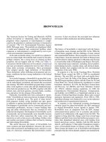
The third is the meteorological network, and the fourth is
the meteorological algorithm or mathematical formula that
describes how the source input is transformed into observed
values of concentration at the receptors (see Figure 1). The
difference between what is actually happening in the atmo-
sphere and what we think happens, based on our measured
C021_001_r03.indd 1163C021_001_r03.indd 1163 11/18/2005 1:31:34 PM11/18/2005 1:31:34 PM
© 2006 by Taylor & Francis Group, LLC
1164 URBAN AIR POLLUTION MODELING
sources and imperfect mathematical formulations as well as
our imperfect sampling of air pollution levels, causes dis-
crepancies between the observed and calculated values. This
makes the verification procedure a very important step in the
development of an urban air pollution model. The remain-

der of this chapter is devoted to these four components, the
verification procedures, and recent research in urban air pol-
lution modeling.
Accounts may be found in the literature of a number of
investigations that do not have the four components of the
mathematical urban air pollution model mentioned above,
namely the source inventory, the mathematical algorithm,
the meteorological network, and the monitoring network.
Some of these have one or more of the components miss-
ing. An example of this kind is the theoretical investigation,
such as that of Lucas (1958), who developed a mathematical
technique for determining the pollution levels of sulfur diox-
ide produced by the thousands of domestic fires in a large
city. No measurements are presented to support this study.
Another is that of Slade (1967), which discusses a megalop-
olis model. Smith (1961) also presented a theoretical model,
which is essentially an urban box model. Another is that of
Bouman and Schmidt (1961) on the growth of pollutant con-
centrations in the cities during stable conditions. Three case
studies, each based on data from a different city, are pre-
sented to support these theoretical results. Studies relevant
to the urban air pollution problem are the pollution surveys
such as the London survey (Commins and Waller,

1967), the
Japanese survey (Canno et al., 1959), and that of the capital
region in Connecticut (Yocum

et al., 1967). In these studies,
analyses are made of pollution measurements, and in some

cases meteorological as well as source inventory informa-
tion are available, but in most cases, the mathematical algo-
rithm for predicting pollution is absent. Another study of this
type is one on suspended particulate and iron concentrations
in Windsor, Canada, by Munn et al. (1969). Early work on
forecasting urban pollution is described in two papers: one
by Scott (1954) for Cleveland, Ohio, and the other by Kauper
et al. (1961) for Los Angeles, California. A comparison of
urban models has been made by Wanta (1967) in his refresh-
ing article that discusses the relation between meteorology
and air pollution.
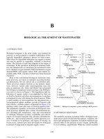
THE SOURCE INVENTORY
In the development of an urban air pollution model two
types of sources are considered: (1) individual point sources,
and (2) distributed sources. The individual point sources are
often large power-generating station stacks or the stacks of
large buildings. Any chimney stack may serve as a point
source, but some investigators have placed lower limits on
the emission rate of a stack to be considered a point source
in the model. Fortak (1966), for example, considers a source
an individual point source if it emits 1 kg of SO
2
per hour,
while Koogler et al. (1967) use a 10-kg-per-hour criterion.
In addition, when ground concentrations are calculated from
the emission of an elevated point source, the effective stack
height must be determined, i.e., the actual stack height plus
the additional height due to plume rise.
Level of
uncertainty

Predicting the future
Modelling the science
Describe case
using available data
3
2
1
Evaluation of
model quality
Approximation to urban boundary layer
Representation of flow in urban canopy
Parameterization of roadside building geometry
representative?
Air quality
monitoring data
Meteorological
monitoring data
Modelled past
air quality
Past situation
Traffic
flow
data
precise?
accurate?
Atmospheric Dispersion
Model
Emissions per vehicle
Measured past air
quality

Future prediction
Modelled future air
quality to inform
AQMA declaration
Will climate change?
Will atmospheric oxidation capacity change?
How will traffic flow change?
How fast will new technology be adopted?
Emissions data
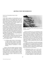
FIGURE 1 Schematic diagram showing flow of data into and out of the atmospheric dispersion model, and three categories
of uncertainty that can be introduced (From Colvile et al., 2002, with permission from Elsevier).
C021_001_r03.indd 1164C021_001_r03.indd 1164 11/18/2005 1:31:34 PM11/18/2005 1:31:34 PM
© 2006 by Taylor & Francis Group, LLC
URBAN AIR POLLUTION MODELING 1165
Information concerning emission rates, emission sched-
ules, or pollutant concentrations is customarily obtained by
means of a source-inventory questionnaire. A municipality
with licensing power, however, has the advantage of being
able to force disclosure of information provided by a source-
inventory questionnaire, since the license may be withheld
until the desired information is furnished. Merely the aware-
ness of this capability is sufficient to result in gratifying
cooperation. The city of Chicago has received a very high
percentage of returns from those to whom a source-inventory
questionnaire was submitted.
Information on distributed sources may be obtained in
part from questionnaires and in part from an estimate of the
population density. Population-density data may be derived
from census figures or from an area survey employing aerial
photography.

In addition to knowing where the sources are, one must
have information on the rate of emission as a function of
time. Information on the emission for each hour would be
ideal, but nearly always one must settle for much cruder
data. Usually one has available for use in the calculations
only annual or monthly emission rates. Corrections for diur-
nal patterns may be applied—i.e., more fuel is burned in
the morning when people arise than during the latter part
of the evening when most retire. Roberts et al. (1970) have
referred to the relationship describing fuel consumption (for
domestic or commercial heating) as a function of time—e.g.,
the hourly variation of coal use—as the “janitor function.”
Consideration of changes in hourly emission patterns with
season is, of course, also essential.
In addition to the classification involving point sources
and distributed sources, the source-inventory information
is often stratified according to broad general categories
to serve as a basis for estimating source strengths. The
nature of the pollutants—e.g., whether sulfur dioxide or
lead—influences the grouping. Frenkiel (1956) described
his sources as those due to: (1) automobiles, (2) oil and gas
heating, (3) incinerators, and (4) industry; Turner (1964)
used these categories: (1) residential, (2) commercial, and
(3) industrial; the Connecticut model (Hilst et al., 1967)
considers these classes: (1) automobiles, (2) home heat-
ing, (3) public services, (4) industrial, and (5) electric
power generally. (Actually, the Connecticut model had a
number of subgroups within these categories.) In general,
each investigator used a classification tailored to his needs
and one that facilitated estimating the magnitude of the

distributed sources. Although source-inventory informa-
tion could be difficult to acquire to the necessary level of
accuracy, it forms an important component of the urban air
pollution model.
MATHEMATICAL EQUATIONS
The mathematical equations of urban air pollution models
describe the processes by which pollutants released to the
atmosphere are dispersed. The mathematical algorithm, the
backbone of any air pollution model, can be conveniently
divided into three major components: (1) the source-emissions
subroutine, (2) the chemical-kinetics subroutine, and (3) the
diffusion subroutine, which includes meteorological param-
eters or models. Although each of these components may
be treated as an independent entity for the analysis of an
existing model, their inferred relations must be considered
when the model is constructed. For example, an exceed-
ingly rich and complex chemical-kinetic subroutine when
combined with a similarly complex diffusion program may
lead to a system of nonlinear differential equations so large
as to preclude a numerical solution on even the largest of
computer systems. Consequently, in the development of the
model, one must “size” the various components and general
subroutines of compatible complexity and precision.
In the most general case, the system to be solved con-
sists of equations of continuity and a mass balance for each
specific chemical species to be considered in the model. For
a concise description of such a system and a cogent devel-
opment of the general solution, see Lamb and Neiburger
(1971).
The mathematical formulation used to describe the

atmospheric diffusion process that enjoys the widest use is a
form of the Gaussian equation, also referred to as the modi-
fied Sutton equation. In its simplest form for a continuous
ground-level point source, it may be expressed as

x
ss
ss
Qu
yz
yz
yz
ϭϪϪ
1
22
2
2
2
2
␲
exp
⎛
⎝
⎜
⎞
⎠
⎟


(1)

where
χ : concentration (g/m
3
)
Q: source strength (g/sec)
u: wind speed at the emission point (m/sec)
σ
y
: perpendicular distance in meters from the center-
line of the plume in the horizontal direction to the point
where the concentration falls to 0.61 times the centerline
value
σ
z
: perpendicular distance in meters from the center-
line of the plume in the vertical direction to the point
where the concentration falls to 0.61 times the center-
line value
x, y, z: spatial coordinates downwind, cross-origin at
the point source
Any consistent system of units may be used.
From an examination of the variables it is readily seen
that several kinds of meteorological measurements are nec-
essary. The wind speed, u, appears explicitly in the equation;
the wind direction is necessary for determining the direction
of pollutant transport from source to receptor.
Further, the values of σ
y
and σ

z
depend upon atmo-
spheric stability, which in turn depends upon the varia-
tion of temperature with height, another meteorological
parameter. At the present time, data on atmospheric stabil-
ity over large urban areas are uncommon. Several authors
have proposed diagrams or equations to determine these
values.
C021_001_r03.indd 1165C021_001_r03.indd 1165 11/18/2005 1:31:35 PM11/18/2005 1:31:35 PM
© 2006 by Taylor & Francis Group, LLC
1166 URBAN AIR POLLUTION MODELING
The temperature variation with height may be obtained
by means of thermal elements mounted on radio or tele-
vision towers. Tethered or free balloons carrying suitable
sensors may also be used. Helicopter soundings of temper-
ature have been used for this purpose in New York City;
Cincinnati, Ohio; and elsewhere. There is little doubt that
as additional effort is devoted to the development of urban
air pollution models, adequate stability measurements will
become available. In a complete study, measurements of
precipitation, solar radiation, and net radiation flux may
be used to advantage. Another meteorological variable of
importance is the hourly temperature for hour-to-hour pre-
dictions, or the average daily temperature for 24-hour cal-
culations. The source strength, Q, when applied to an area
source consisting of residential units burning coal for space
heating, is a direct function of the number of degree-hours
or degree-days. The number of degree-days is defined as
the difference between the average temperature for the
day and 65Њ. If the average temperature exceeds 65Њ, the

degree-day value is considered zero. An analogous defi-
nition applies for the degree-hour. Turner (1968) points
out that in St. Louis the degree-day or degree-hour values
explain nearly all the variance of the output of gas as well
as of steam produced by public utilities.
THE USE OF GRIDS
In the development of a mathematical urban air pollution
model, two different grids may be used: one based on exist-
ing pollution sources and the other on the location of the
instruments that form the monitoring network.
The Pollution-Source Grid
In the United States, grid squares 1 mile on a side are frequently
used, such as was done by Davidson,

Koogler, and Turner.
Fortak, of West Germany, used a square 100 ϫ 100 m. The
Connecticut model is based on a 5000-ft grid, and Clarke’s


Cincinnati model on sectors of a circle. Sources of pollution
may be either point sources, such as the stacks of a public
utility, or distributed sources, such as the sources represent-
ing the emission of many small homes in a residential area.
The Monitoring Grid
In testing the model, one resorts to measurements obtained
by instruments at monitoring stations. Such monitoring sta-
tions may also be located on a grid. Furthermore, this grid
may be used in the computation of concentrations by means
of the mathematical equation—e.g., concentrations are cal-
culated for the midpoints of the grid squares. The emission

grid and monitoring grid may be identical or they may be
different. For example, Turner

used a source grid of 17 ϫ
16 miles, but a measurement grid of 9 ϫ 11 miles. In the
Connecticut model, the source grid covers the entire state,
and calculations based on the model also cover the entire
state. Fortak

used 480 ϫ 800-m rectangles.
TYPES OF URBAN AIR POLLUTION MODELS
Source-Oriented Models
In applying the mathematical algorithm, one may proceed
by determining the source strength for a given point source
and then calculating the isopleths of concentration down-
wind arising from this source. The calculation is repeated
for each area source and point source. Contributions made
by each of the sources at a selected point downwind are then
summed to determine the calculated value of the concentra-
tion. Isopleths of concentration may then be drawn to pro-
vide a computed distribution of the pollutants.
In the source-oriented model, detailed information is
needed both on the strength and on the time variations of
the source emissions. The Turner model (1964) is a good
example of a source-oriented model.
It must be emphasized that each urban area must be
“calibrated” to account for the peculiar characteristics of
the terrain, buildings, forestation, and the like. Further, local
phenomena such as lake or sea breezes and mountain-valley
effects may markedly influence the resulting concentrations;

for example, Knipping and Abdub (2003) included sea-salt
aerosol in their model to predict urban ozone formation.
Specifically, one would have to determine such relations as
the variations of σ


y


and σ


z


with distance or the magnitude of
the effective stack heights. A network of pollution-monitoring
stations is necessary for this purpose. The use of an algorithm
without such a calibration is likely to lead to disappointing
results.
Receptor-Oriented Models
Several types of receptor-oriented models have been devel-
oped. Among these are: the Clarke model, the regression
model, the Argonne tabulation prediction scheme, and the
Martin model.
The Clarke Model
In the Clarke model (Clarke, 1964), one of the most well
known, the receptor or monitoring station is located at the
center of concentric circles having radii of 1, 4, 10, and 20 km
respectively. These circles are divided into 16 equal sec-

tors of 22 1/2Њ. A source inventory is obtained for each of
the 64 (16 ϫ 4) annular sectors. Also, for the 1-km-radius
circle and for each of the annular rings, a chart is prepared
relating x/Q (the concentration per unit source strength)
and wind speed for various stability classes and for vari-
ous mixing heights. In refining his model, Clarke (1967)
considers separately the contributions to the concentration
levels made by transportation, industry and commerce,
space heating, and strong-point sources such as utility
stacks. The following equations are then used to calculate
the pollutant concentration.

␹␹
T
Ti
i
Ti
Qϭ
ϭ
Q
(
)
∑
1
4
C021_001_r03.indd 1166C021_001_r03.indd 1166 11/18/2005 1:31:35 PM11/18/2005 1:31:35 PM
© 2006 by Taylor & Francis Group, LLC
URBAN AIR POLLUTION MODELING 1167

␹␹

I
Ii
i
Ii
QQϭ
ϭ
(
)
∑
1
4

␹␹
S
Si
i
Si
QQϭ
ϭ
(
)
∑
1
4


␹␹␹␹ ␹
Total
ϭϩϩϩ
ϭ

abc k
TIS i
i
p
1
4
∑
where
␹ : concentration (g/m
3
)
Q: source strength (g/sec)
T: subscript to denote transportation sources
I: subscript to denote industrial and commercial
sources
S: subscript to denote space-heating sources
p: subscript to denote point sources
i: refers to the annular sectors
The above equations with some modification are taken
from Clarke’s report (1967). Values of the constants a, b, and
c can be determined from information concerning the diur-
nal variation of transportation, industrial and commercial,
and space-heating sources. The coefficient k
i
represents a
calibration factor applied to the point sources.
The Linear Regression-Type Model
A second example of the receptor-oriented model is one
developed by Roberts and Croke (Roberts et al., 1970)

using
regression techniques. Here,
␹ϭ ϩ ϩ ϩ
ϭ
CCQCQ kQ
ii
i
n
01122
1
∑
In applying this equation, it is necessary first to stratify
the data by wind direction, wind speed, and time of day.
C
0
represents the background level of the pollutant; Q
1

represents one type of source, such as commercial and
industrial emissions; and Q
2
may represent contributions
due to large individual point sources. It is assumed that
there are n point sources. The coefficients C
1
and C
2
and k
i

represent the 1/ s
y
s
z
term as well as the contribution of the
exponential factor of the Gaussian-type diffusion equation
(see Equation 1).
Multiple discriminant analysis techniques for indi-
vidual monitoring stations may be used to determine
the probability that pollutant concentrations fall within
a given range or that they exceed a given critical value.
Meteorological variables, such as temperature, wind
speed, and stability, are used as the independent variable
in the discriminant function.
The Martin Model
A diffusion model specifically suited to the estimation
of long-term average values of air quality was developed
by Martin (1971). The basic equation of the model is the
Gaussian diffusion equation for a continuous point source. It
is modified to allow for a multiplicity of point sources and a
variety of meteorological conditions.
The model is receptor-oriented. The equations for the
ground-level concentration within a given 22 1/2Њ sector
at the receptor for a given set of meteorological conditions
(i.e., wind speed and atmospheric stability) and a specified
source are listed in his work. The assumption is made that
all wind directions within a 22 1/2Њ sector corresponding to
a 16-point compass occur with equal probability.
In order to estimate long-term air quality, the single-
point-source equations cited above are evaluated to deter-

mine the contribution from a given source at the receptor for
each possible combination of wind speed and atmospheric
stability. Then, using Martin’s notation, the long-term aver-
age is given by
␹ϭ FD LS LS
nn
SLN
(, ,,)(,)xr
∑∑∑

where D
n
indicates the wind-direction sector in which transport
from a particular source ( n ) to the receptor occurs; r
n
is the
distance from a particular source to the receptor; F ( D
n
, L, S )
denotes the relative frequency of winds blowing into the given
wind-direction sector ( D
n
) for a given wind-speed class ( S ) and
atmospheric stability class ( L ); and N is the total number of
sources. The joint frequency distribution F ( D
n
, L, S ) is deter-
mined by the use of hourly meteorological data.
A system of modified average mixing heights based on
tabulated climatological values is developed for the model.

In addition, adjustments are made in the values of some
mixing heights to take into account the urban influence.
Martin has also incorporated the exponential time decay of
pollutant concentrations, since he compared his calculations
with measured sulfur-dioxide concentrations for St. Louis,
Missouri.
The Tabulation Prediction Scheme
This method, developed at the Argonne National Laboratory,
consists of developing an ordered set of combinations of rel-
evant meteorological variables and presenting the percentile
distribution of SO
2
concentrations for each element in the
set. In this table, the independent variables are wind direc-
tion, hour of day, wind speed, temperature, and stability. The
10, 50, 75, 90, 98, and 99 percentile values are presented
as well as the minimum and the maximum values. Also
presented are the interquartile range and the 75 to 95 per-
centile ranges to provide measures of dispersion and skew-
ness, respectively. Since the meteorological variables are
ordered, it is possible to look up any combination of meteo-
rological variables just as one would look up a name in a
telephone book or a word in a dictionary. This method, of
C021_001_r03.indd 1167C021_001_r03.indd 1167 11/18/2005 1:31:35 PM11/18/2005 1:31:35 PM
© 2006 by Taylor & Francis Group, LLC
1168 URBAN AIR POLLUTION MODELING
course, can be applied only as long as the source distribu-
tion and terrain have not changed appreciably. For contin-
ued use of this method, one must be cognizant of changes
in the sources as well as changes in the terrain due to new

construction.
In preparing the tabulation, the data are first stratified
by season and also by the presence or absence of precipita-
tion. Further, appropriate group intervals must be selected
for the meteorological variables to assure that within each
grouping the pollution values are not sensitive to changes
in that variable. For example, of the spatial distribution of
the sources, one finds that the pollution concentration at a
station varies markedly with changes in wind direction. If
one plots percentile isopleths for concentration versus wind
direction, one may choose sectors in which the SO
2
concen-
trations are relatively insensitive to direction change. With
the exception of wind direction and hour of day, the meteo-
rological variables of the table vary monotonically with SO
2

concentration. The tabulation prediction method has advan-
tages over other receptor-oriented technique in that (1) it is
easier to use, (2) it provides predictions of pollution con-
centrations more rapidly, (3) it provides the entire percentile
distribution of pollutant concentration to allow a forecaster
to fine-tune his prediction based on synoptic conditions, and
(4) it takes into account nonlinearities in the relationships
of the meteorological variables and SO
2
concentrations. In
a sense, one may consider the tabulation as representing a
nonlinear regression hypersurface passing through the data

that represents points plotted in n -dimensional space. The
analytic form of the hypersurface need not be determined in
the use of this method.
The disadvantages of this method are that (1) at least
2 years of meteorological data are necessary, (2) changes in
the emission sources degrade the method, and (3) the model
could not predict the effect of adding, removing, or modify-
ing important pollution sources; however, it can be designed
to do so.
Where a network of stations is available such as exists in
New York City, Los Angeles, or Chicago, then the receptor-
oriented technique may be applied to each of the stations
to obtain isopleths or concentration similar to that obtained
in the source-oriented model. It would be ideal to have a
source-oriented model that could be applied to any city,
given the source inventory. Unfortunately, the nature of the
terrain, general inaccuracies in source-strength information,
and the influence of factors such as synoptic effect or the
peculiar geometries of the buildings produce substantial
errors. Similarly, a receptor-oriented model, such as the
Clarke model or one based on regression techniques, must
be tailored to the location. Every urban area must therefore
be calibrated, whether one desires to apply a source-oriented
model or a tabulation prediction scheme. The tabulation pre-
diction scheme, however, does not require detailed informa-
tion on the distribution and strength of emission sources.
Perhaps the optimum system would be one that would
make use of the advantages of both the source-oriented
model, with its prediction capability concerning the effects
of changes in the sources, and the tabulation prediction

scheme, which could provide the probability distributions
of pollutant concentrations. It appears possible to develop
a hybrid system by developing means for appropriately
modifying the percentile entries when sources are modified,
added, or removed. The techniques for constructing such a
system would, of course, have general applicability.
The Fixed-Volume Trajectory Model
In the trajectory model, the path of a parcel of air is predicted
as it is acted upon by the wind. The parcel is usually con-
sidered as a fixed-volume chemical reactor with pollutant
inputs only from sources along its path; in addition, various
mathematical constraints placed on mass transport into and
out of the cell make the problem tractable. Examples of this
technique are discussed by Worley (1971). In this model,
derived pollution concentrations are known only along the
path of the parcel considered. Consequently, its use is limited
to the “strategy planning” problem. Also, initial concentra-
tions at the origin of the trajectory and meteorological vari-
ables along it must be well known, since input errors along
the path are not averageable but, in fact, are propagated.
The Basic Approach
Attempts have been made to solve the entire system of three-
dimensional time-dependent continuity equations. The ever-
increasing capability of computer systems to handle such
complex problems easily has generally renewed interest in this
approach. One very ambitious treatment is that of Lamb and
Neiburger (1971),

who have applied their model to carbon-
monoxide concentrations in the Los Angeles basin. However,

chemical reactions, although allowed for in their general for-
mulation, are not considered because of the relative inertness
of CO. Nevertheless, the validity of the diffusion and emission
subroutines is still tested by this procedure.
The model of Friedlander

and Seinfeld (1969) also
considers the general equation of diffusion and chemical
reaction. These authors extend the Lagrangian similarity
hypothesis to reacting species and develop, as a result, a
set of ordinary differential equations describing a variable-
volume chemical reactor. By limiting their chemical system
to a single irreversible bimolecular reaction of the form
A ϩ B ϩ C, they obtain analytical solutions for the ground-
level concentration of the product as a function of the mean
position of the pollution cloud above ground level. These
solutions are also functions of the appropriate meteorologi-
cal variables, namely solar radiation, temperature, wind con-
ditions, and atmospheric stability.
ADAPTATION OF THE BASIC EQUATION TO
URBAN AIR POLLUTION MODELS
The basic equation, (1), is the continuous point-source equa-
tion with the source located at the ground. It is obvious that the
sources of an urban complex are for the most part located above
the ground. The basic equation must, therefore, be modified
C021_001_r03.indd 1168C021_001_r03.indd 1168 11/18/2005 1:31:35 PM11/18/2005 1:31:35 PM
© 2006 by Taylor & Francis Group, LLC
URBAN AIR POLLUTION MODELING 1169
to represent the actual conditions. Various authors have
proposed mathematical algorithms that include appropriate

modifications of Equation (1). In addition, a source-oriented
model developed by Roberts et al. (1970) to allow for time-
varying sources of emission is discussed below; see the section
“Time-Dependent Emissions (the Roberts Model).”
Chemical Kinetics: Removal or Transformation
of Pollutants
In the chemical-kinetics portion of the model, many differ-
ent approaches, ranging in order from the extremely simple
to the very complex, have been tried. Obviously the simplest
approach is to assume no chemical reactions are occurring at
all. Although this assumption may seem contradictory to our
intent and an oversimplification, it applies to any pollutant
that has a long residence time in the atmosphere. For exam-
ple, the reaction of carbon monoxide with other constituents
of the urban atmosphere is so small that it can be considered
inert over the time scale of the dispersion process, for which
the model is valid (at most a few hours).
Considerable simplification of the general problem can
be effected if chemical reactions are not included and all vari-
ables and parameters are assumed to be time-independent
(steady-state solution). In this instance, a solution is obtained
that forms the basis for most diffusion models: the use of the
normal bivariate or Gaussian distribution for the downwind
diffusion of effluents from a continuous point source. Its use
allows steady-state concentrations to be calculated both at
the ground and at any altitude. Many modifications to the
basic equation to account for plume rise, elevated sources,
area sources, inversion layers, and variations in chimney
heights have been proposed and used. Further discussion of
these topics is deferred to the following four sections.

The second level of pseudo-kinetic complexity assumes
first-order or pseudo-first-order reactions are responsible for
the removal of a particular pollutant; as a result, its concentra-
tion decays exponentially with time. In this case, a characteris-
tic residence time or half-life describes the temporal behavior
of the pollutant. Often, the removal of pollutants by chemical
reaction is included in the Gaussian diffusion model by simply
multiplying the appropriate diffusion equation by an exponen-
tial term of the form exp(− t / T ), where T represents the half-life
of the pollutant under consideration. Equations employing this
procedure are developed below. The interaction of sulfur diox-
ide with other atmospheric constituents has been treated in this
way by many investigators; for examples, see Roberts et al.
(1970) and Martin (1971). Chemical reactions are not the only
removal mechanism for pollutant. Some other processes con-
tributing to their disappearance may be absorption by plants,
soil-bacteria action, impact or adsorption on surfaces, and
washout (for example, see Figure 2

). To the extent that these
processes are simulated by or can be fitted to an exponential
decay, the above approximation proves useful and valid.
These three reactions appear in almost every chemical-
kinetic model. On the other hand, many different sets of equa-
tions describing the subsequent reactions have been proposed.
For example, Hecht and Seinfeld (1972) recently studied the
propylene-NO-air system and list some 81 reactions that can
occur. Any attempt to find an analytical solution for a model
utilizing all these reactions and even a simple diffusion sub-
model will almost certainly fail. Consequently, the number of

equations in the chemical-kinetic subroutine is often reduced
by resorting to a “lumped parameter” stratagem. Here, three
general types of chemical processes are identified: (1) a chain-
initiating process involving the inorganic reactions shown
above as well as subsequent interactions of product oxidants
with source and product hydrocarbons, to yield (2) chain-
propagating reactions in which free radicals are produced;
these free radicals in turn react with the hydrocarbon mix to
produce other free radicals and organic compounds to oxide
NO to NO
2
, and to participate in (3) chain-terminating reac-
tions; here, nonreactive end products (for example, peroxy-
acetylnitrate) and aerosol production serve to terminate the
chain. In the lumped-parameter representation, reaction-
rate equations typical of these three categories (and usually
selected from the rate-determining reactions of each category)
are employed, with adjusted rate constants determined from
appropriate smog-chamber data. An attempt is usually made
to minimize the number of equations needed to fit well a large
sample of smog-chamber data. See, for examples, the studies
of Friedlander

and Seinfeld (1969) and Hecht and Seinfeld
(1972). Lumped parameter subroutines are primarily designed
to simulate atmospheric conditions with a simplified chemical-
kinetic scheme in order to reduce computing time when used
with an atmospheric diffusion model.
Elevated Sources and Plume Rise
When hot gases leave a stack, the plume rises to a certain

height dependent upon its exit velocity, temperature, wind
speed at the stack height, and atmospheric stability. There
are several equations used to determine the total or virtual
height at which the model considers the pollutants to be
emitted. The most commonly used is Holland’s equation:
⌬H
v
u
P
TT
T
d
ssa
a
ϭϩϫ
Ϫ
15 268 10
2
()
−
⎛
⎝
⎜
⎞
⎠
⎟
⎛
⎝
⎜
⎞

⎠
⎟
⎡
⎣
⎢
⎢
⎤
⎦
⎥
⎥
where
∆ H: plume rise
v
s
: stack velocity (m/sec)
d: stack diameter (m)
u: wind speed (m/sec)


P: pressure (kPa)
T
s
: gas exit temperature (K)
T
a
: air temperature (K)
The virtual or effective stack height is
H ϭ h ϩ ∆ H
where
H: effective stack height

h: physical stack height
C021_001_r03.indd 1169C021_001_r03.indd 1169 11/18/2005 1:31:35 PM11/18/2005 1:31:35 PM
© 2006 by Taylor & Francis Group, LLC
1170 URBAN AIR POLLUTION MODELING
With the origin of the coordinate system at the ground, but
the source at a height H, Equation (2) becomes

␹
Qu
yzH t
T
yz
yz
ϭϪϪ
Ϫ
Ϫ
1
22
0 693
2
2
2
2
pss
ss
exp
()
exp
.
⎛

⎝
⎜
⎞
⎠
⎟
⎛
⎝
⎜
⎞
⎠
⎟
1/2

(3)

Mixing of Pollutants under an Inversion Lid
When the lapse rate in the lowermost layer, i.e., from the
ground to about 200 m, is near adiabatic, but a pronounced
inversion exists above this layer, the inversion is believed to
act as a lid preventing the upward diffusion of pollutants. The
pollutants below the lid are assumed to be uniformly mixed.
By integrating Equation (3) with respect to z and distributing
the pollutants uniformly over a height H, one obtains
␹
QuH
yt
T
y
y
ϭϪϪ

1
2
0 693
2
2
ps
s
exp exp
.
⎛
⎝
⎜
⎞
⎠
⎟
⎛
⎝
⎜
⎞
⎠
⎟
1/2

Those few measurements of concentration with height that
do exist do not support the assumption that the concentra-
tion is uniform in the lowermost layer. One is tempted to
say that the mixing-layer thickness, H, may be determined
by the height of the inversion; however, during transitional
conditions, i.e., at dawn and dusk, the thickness of the layer
containing high concentrations of pollutants may differ from

that of the layer from the ground to the inversion base.
The thermal structure of the lower layer as well as pollut-
ant concentration as a function of height may be determined
by helicopter or balloon soundings.
The Area Source
When pollution arises from many small point sources such
as small dwellings, one may consider the region as an area
source. Preliminary work on the Chicago model indicates
that contribution to observed SO
2
levels in the lowest tens of
feet is substantially from dwellings and exceeds that emanat-
ing from tall stacks, such as power-generating stacks. For
a rigorous treatment, one should consider the emission Q
as the emission in units per unit area per second, and then
integrate Q along x and along y for the length of the square.
Downwind, beyond the area-source square, the plume may
be treated as originating from a point source. This point
source is considered to be at a virtual origin upwind of the
area-source square. As pointed out by Turner,

the approxi-
mate equation for an area source can be calculated as
␹
Q
y
xx
zh t
T
yy

z
ϭ
Ϫ
ϩ
Ϫ
Ϫ
Ϫexp
(
exp
.
2
2
0
2
2
2
2
2
0 693
s
s
()
⎡
⎣
⎤
⎦
⎛
⎝
⎜
⎜

⎞
⎠
⎟
⎟
)
1/2
⎛⎛
⎝
⎜
⎞
⎠
⎟
()
⎡
⎣
⎤
⎦
ps
s
uxx
yy z0
ϩ
where σ
y
( x
y

0
ϩ x ) represents the standard deviation of the
horizontal crosswind concentration as a function of the dis-

tance x
y

0
ϩ x from the virtual origin. Since the plume is con-
sidered to extend to the point where the concentration falls
to 0.1 that of the centerline concentration, σ
y
( x
y

0
) ϭ S /403
where σ
y
( x
y

0
) is the standard deviation of the concentration
at the downwind side of the square of side length S . The
distance x
y

0
from the virtual origin to the downwind side of
the grid square may be determined, and is that distance for
which σ
y
( x

y 0
) ϭ S /403. The distance x is measured from the
downwind side of the grid square. Other symbols have been
previously defined.
Correction for Variation in Chimney Heights
for Area Sources
In any given area, chimneys are likely to vary in height above
ground, and the plume rises vary as well. The variation of
effective stack height may be taken into account in a manner
similar to the handling of the area source. To illustrate, visu-
alize the points representing the effective stack height pro-
jected onto a plane perpendicular to the ground and parallel
both to two opposite sides of the given grid square and to the
horizontal component of the wind vector. The distribution
of the points on this projection plane would be similar to the
distribution of the sources on a horizontal plane.
Based on Turner’s discussion (1967), the equation for an
area source and for a source having a Gaussian distribution
of effective chimney heights may be written as
␹
Q
y
xx
zh
xx
yy
zz
ϭ
Ϫ
ϩ

Ϫ
Ϫ
ϩ
Ϫexp exp
2
0
2
2
0
2
2
2
s
s
()
⎡
⎣
⎤
⎦
(
)
()
⎡
⎣
⎤
⎦
⎛
⎝
⎜
⎜

⎞
⎠
⎟
⎟
00 693
0
. t
T
uxx xx
yy zz
1/2
0
⎛
⎝
⎜
⎞
⎠
⎟
()
⎡
⎣
⎤
⎦
()
⎡
⎣
⎤
⎦
ps sϩϩ

where σ
z
( x
z

0
ϩ x ) represents the standard deviation of the
vertical crosswind concentration as a function of the dis-
tance x
z

0
ϩ x from the virtual origin. The value of σ
z
( x
z 0
) is
arbitrarily chosen after examining the distribution of effec-
tive chimney heights, and the distance x
z

0
represents the dis-
tance from the virtual origin to the downwind side of the grid
square. The value x
z 0
may be determined and represents the
distance corresponding to the value for σ
z
( x

z

0
). The value of
x
y

0

usually differs from that of x
z

0
. The other symbols retain
their previous definition.
In determining the values of σ
y
( x
y

0
ϩ x ) and σ
z
( x
z 0
ϩ x ), one
must know the distance from the source to the point in question
or the receptor. If the wind direction changes within the aver-
aging interval, or if there is a change of wind direction due to
local terrain effects, the trajectories are curved. There are sev-

eral ways of handling curved trajectories. In the Connecticut
model, for example, analytic forms for the trajectories were
developed. The selection of appropriate trajectory or stream-
line equations (steady state was assumed) was based on the
C021_001_r03.indd 1170C021_001_r03.indd 1170 11/18/2005 1:31:35 PM11/18/2005 1:31:35 PM
© 2006 by Taylor & Francis Group, LLC
URBAN AIR POLLUTION MODELING 1171
wind and stability conditions. In the St. Louis model, Turner


developed a computer program using the available winds to
provide pollutant trajectories. Distances obtained from the tra-
jectories are then used in the Pasquill diagrams or equations to
determine the values of σ
y
( x
y 0
ϩ x ) and σ
z
( x
z

0
ϩ x ).
Time-Dependent Emissions (The Roberts Model)
The integrated puff transport algorithm of Roberts et al.
(1970), a source-oriented model, uses a three-dimensional
Gaussian puff kernel as a basis. It is designed to simulate the
time-dependent or transient emissions from a single source.
Concentrations are calculated by assuming that dispersion

occurs from Gaussian diffusion of a puff whose centroid
moves with the mean wind. Time-varying source emissions
as well as variable wind speeds and directions are approxi-
mated by a time series of piecewise continuous emission and
meteorological parameters. In addition, chemical reactions
are modeled by the inclusion of a removal process described
by an exponential decay with time.
The usual approximation for inversion lids of constant
height, namely uniform mixing arising from the superpo-
sition of an infinite number of multiple source reflections,
is made. Additionally, treatments for lids that are steadily
rising or steadily falling and the fumigation phenomenon are
incorporated.
The output consists of calculated concentrations for a
given source for each hour of a 24-hour period. The concen-
trations can be obtained for a given receptor or for a uniform
horizontal or vertical grid up to 1000 points.
The preceding model also forms the basis for two other
models, one whose specific aim is the design of optimal
control strategies, and a second that repetitively applies the
single-source algorithm to each point and area source in the
model region.
METEOROLOGICAL MEASUREMENTS
Wind speed and direction data measured by weather bureaus are
used by most investigators, even though some have a number
of stations and towers of their own. Pollutants are measured
for periods of 1 hour, 2 hours, 12 hours, or 24 hours. 12- and
24-hour samples of pollutants such as SO
2
leave much to be

desired, since many features of their variations with time are
obscured. Furthermore, one often has difficulty in determining
a representative wind direction or even a representative wind
speed for such a long period.
The total amount of data available varies considerably in
the reviewed studies. Frenkiel’s study (1956)

was based on
data for 1 month only. A comparatively large amount of data
was gathered by Davidson (1967),

but even these in truth
represent a small sample. One of the most extensive studies
is the one carried out by the Argonne National Laboratory
and the city of Chicago in which 15-minute readings of SO
2

for 8 stations and wind speed and direction for at least 13
stations are available for a 3-year period.
In the application of the mathematical equations, one is
required to make numerous arbitrary decisions: for example,
one must choose the way to handle the vertical variation of
wind with height when a high stack, about 500 ft, is used as
a point source; or how to test changes in wind direction or
stability when a change occurs halfway through the 1-hour
or 2-hour measuring period. In the case of an elevated point
source, Turner

in his St. Louis model treated the plume as one
originating from the point source up to the time of a change in

wind direction and as a combination of an instantaneous line
puff and a continuous point source thereafter. The occurrence
of precipitation presents serious problems, since adequate
diffusion measurements under these conditions are lacking.
Furthermore, the chemical and physical effects of precipita-
tion on pollutants are only poorly understood. In carrying
forward a pollutant from a source, one must decide on how
long to apply the calculations. For example, if a 2-mph wind is
present over the measuring grid and a source is 10 miles away,
one must take account of the transport for a total of 5 hours.
Determining a representative wind speed and wind direc-
tion over an urban complex with its variety of buildings and
other obstructions to the flow is frequently difficult, since
the horizontal wind field is quite heterogeneous. This is so
for light winds, especially during daytime when convective
processes are taking place. With light-wind conditions, the
wind direction may differ by 180Њ within a distance of 1 mile.
Numerous land stations are necessary to depict the true wind
field. With high winds, those on the order of 20 mph, the
wind direction is quite uniform over a large area, so that
fewer stations are necessary.


METHODS FOR EVALUATING URBAN AIR
POLLUTION MODELS
To determine the effectiveness of a mathematical model,
validation tests must be applied. These usually include a
comparison of observed and calculated values. Validation
tests are necessary not only for updating the model because
of changes in the source configuration or modification in

terrain characteristics due to new construction, but also for
comparing the effectiveness of the model with any other that
may be suggested. Of course, the primary objective is to see
how good the model really is, both for incident control as
well as for long-range planning.
Scatter Plots and Correlation Measures
Of the validation techniques appearing in the literature, the
most common involves the preparation of a scatter diagram
relating observed and calculated values ( Y
obs
vs. Y
calc
).

The
degree of scatter about the Y
obs
ϭ Y
calc
line provides a mea-
sure of the effectiveness of the model. At times, one finds
that a majority of the points lies either above the line or
below the line, indicating systematic errors.
It is useful to determine whether the model is equally
effective at all concentration levels. To test this, the calcu-
lated scale may be divided into uniform bandwidths and the
C021_001_r03.indd 1171C021_001_r03.indd 1171 11/18/2005 1:31:36 PM11/18/2005 1:31:36 PM
© 2006 by Taylor & Francis Group, LLC
1172 URBAN AIR POLLUTION MODELING
mean square of the deviations abou t the Y

obs
ϭ Y
calc
line cal-
culated for each bandwidth. Another test for systematic error
as a function of bandwidth consists of an examination of the
mean of the difference between calculated and observed
values for Y
calc
Ͻ Y
obs
and similarly for Y
calc
Ͼ Y
obs
.
The square of the linear correlation coefficient between
calculated and observed values or the square of the correla-
tion ratio for nonlinear relationships represent measures of
the effectiveness of the mathematical equation. For a linear
relationship between the dependent variable, e.g., pollutant
concentration, and the independent variables,
R
SS
y
y
yy
y
2
2

2
2
11ϭϪϭϪϭ
Ϫ
s
s
s
unexplained variance
total variance
2
22
explained variance
total variance
ϭ

where
R
2
: square of the correlation coefficient between
observed and calculated values
S
y

2
: average of the square of the deviations about the
regression line, plane, or hyperplane
σ
y

2

: variance of the observed values
Statistical Analysis
Several statistical parameters can be calculated to evaluate
the performance of a model. Among those commonly used
for air pollution models are Kukkonen, Partanen, Karppinen,
Walden, et al. (2003); Lanzani and Tamponi (1995):
The index of agreement
IA = 1
2
2
Ϫ
Ϫ
ϪϩϪ
()
[| | | |]
CC
CC CC
po
po oo

R
R
CCCC
oopp
op
ϭ
ϪϪ()()
ss
⎡
⎣

⎢
⎢
⎤
⎦
⎥
⎥

The bias
Biasϭ
ϪCC
C
po
o
The fractional bias
FBϭ
Ϫ
ϩ
CC
CC
po
po
05.( )

The normalized mean of the square of the error
NMSE ϭ
Ϫ()CC
CC
po
po
2

where
C
p
: predicted concentrations
C
o
: predicted observed concentrations
σ
o
: standard deviation of the observations
σ
p
:

standard deviation of the predictions
The overbar concentrations refer to the average overall values.
The parameters IA and R
2
are measures of the correla-
tion of two time series of values, the bias is a measurement of
the overall tendency of the model, the FB is a measure of the
agreement of the mean values, and the NMSE is a normalized
estimation of the deviation in absolute value.
The IA varies from 0.0 to 1.0 (perfect agreement between
the observed and predicted values). A value of 0 for the
bias, FB, or NMSE indicates perfect agreement between the
model and the data.
Thus there are a number of ways of presenting the results
of a comparison between observed and calculated values and
of calculating measures of merit. In the last analysis the effec-

tiveness of the model must be judged by how well it works to
provide the needed information, whether it will be used for
day-to-day control, incident alerts, or long-range planning.
RECENT RESEARCH IN URBAN AIR POLLUTION
MODELING
With advances in computer technology and the advent of new
mathematical tools for system modeling, the field of urban
air pollution modeling is undergoing an ever-increasing
level of complexity and accuracy. The main focus of recent
research is on particles, ozone, hydrocarbons, and other
substances rather than the classic sulfur and nitrogen com-
pounds. This is due to the advances in technology for pollu-
tion reduction at the source. A lot of attention is being devoted
to air pollution models for the purpose of urban planning
and regulatory- standards implementation. Simply, a model
can tell if a certain highway should be constructed without
increasing pollution levels beyond the regulatory maxima or
if a new regulatory value can be feasibly obtained in the time
frame allowed. Figure 2 shows an example of the distribution
of particulate matter (PM
10
) in a city. As can be inferred, the
presence of particulate matter of this size is obviously a traffic-
related pollutant.
Also, some modern air pollution models include meteo-
rological forecasting to overcome one of the main obstacles
that simpler models have: the assumption of average wind
speeds, direction, and temperatures.
At street level, the main characteristic of the flow is the
creation of a vortex that increases concentration of pollut-

ants on the canyon side opposite to the wind direction, as
C021_001_r03.indd 1172C021_001_r03.indd 1172 11/18/2005 1:31:36 PM11/18/2005 1:31:36 PM
© 2006 by Taylor & Francis Group, LLC
URBAN AIR POLLUTION MODELING 1173
FIGURE 2 Predicted spatial distribution of the yearly means of PM
10
in central Helsinki
in 1998 (mg/m
3
). The white star indicates the predicted maximum concentration in the
area (40.4 mg/m
3
) (From Kukkonen et al., 2001, with permission from Elsevier).
shown in Figure 3

(Berkowicz, 2000a). The Danish opera-
tional street pollution model (OSPM) has been used by sev-
eral researchers to model dispersion of pollutants at street
level. Several studies have assessed the validity of the model
by using data for different cities in Europe.
New techniques such as Fuzzy Logic and Neural
Networks

have been used with great results (Kukkonen,
Partanen, Karppinen, Ruuskanen, et al., 2003; Viotti et al.,
2002, Pokrovskya et al., 2002; Pelliccioni and Poli, 2002).
Schlink and Volta (2000) used grey box stochastic models
and extended autoregressive moving average models to
predict ozone formation. Other approaches have been time-
series analysis, regression analysis, and statistical modeling,

among others.
For additional information, the reader is referred to the
references at the end of the chapter.
CONCLUDING REMARKS
Inadequacies and shortcomings exist in our assessment of
each of the components of the mathematical urban air pollu-
tion model. In this section these difficulties are discussed.
The Source Inventory
For large metropolitan areas, one finds that the inventory
obtained by the usual methods, such as questionnaires, is
often out of date upon its completion. Continuous updat-
ing is necessary. However, in a receptor-oriented model,
the requirement for a detailed source inventory is relaxed.
Further, by developing a receptor-oriented “anomaly” model,
one may further reduce the error resulting from inadequate
source information. In the anomaly-type model, changes in
the dependent variable over a given time period are calcu-
lated. This interval may be 1, 2, 4, or 6 hours.
Initial Mixing
According to Schroeder and Lane (1988), “Initial mixing
refers to the physical processes that act on pollutants imme-
diately after their release from an emission source. The
nature and extent of the initial interaction between pollutants
and the ambient air depend on the actual configuration of the
source in terms of its area, its height above the surrounding
terrain, and the initial buoyancy conditions.”


C021_001_r03.indd 1173C021_001_r03.indd 1173 11/18/2005 1:31:36 PM11/18/2005 1:31:36 PM
© 2006 by Taylor & Francis Group, LLC

1174 URBAN AIR POLLUTION MODELING
Leeward
side
Windward
side
Direct plume
Recirculating air
Background pollution
Roof level wind
FIGURE 3 Schematic illustration of flow and dispersion of pollutants in street
canyons (From Berkowicz, 2000a, with permission of Springer Science and
Business media).
Advection
Transport
Reaction
Net Loss
85
1000 23
22
26
61
26
29
52
21
26
15
14
910
2

4
3
8
2
3
<1
<1
<1
<1
<1
<1
<1
5
SOIL
WATER
SEDIMENT
FILM
AIR
VEG’N
FIGURE 4 Estimated rates of chemical movement and transformation for 2,3,7,8-CL
4
DD based on an emission of 1 mil/
hour into air. Numbers shown are transport rate in mmol/hour (From Diamond et al., 2001, with permission from Elsevier).
C021_001_r03.indd 1174C021_001_r03.indd 1174 11/18/2005 1:31:36 PM11/18/2005 1:31:36 PM
© 2006 by Taylor & Francis Group, LLC
URBAN AIR POLLUTION MODELING 1175
The mixing layer is the lower region of the troposphere
in which pollutants are relatively free to circulate and dis-
perse vertically as well as horizontally because of the pre-
ponderance of small-scale turbulence. It may extend to a

height as small as 50 m or as great as 5 km above the surface
(Deardorff, 1975). More typically, it extends about 1 to 2 km
during the day and a few hundred meters at night, although
day-to-day variations can be quite large (Smith, 1982). This
turbulence promotes intimate contact between vapor-phase
and aerosol-associated pollutants.
Such direct contact is an important step in the chain of
events that ultimately results in chemical transformations
of pollutants near their source before extensive dilution has
occurred and while their air concentrations are still relatively
high. The consequences of limited vertical mixing may be
exacerbated at northern latitudes, where air pollutants released
close to the ground may disperse only to a very limited extent
because of the extreme stability of air brought about by inver-
sion layers characteristic of the Arctic, especially in winter.
This situation can give rise to elevated ambient-air concentra-
tion of noxious contaminants in those regions.
Pollutant Measurements
It is necessary to remember that the distribution of any con-
taminants is a function of space and time. With a heteroge-
neous distribution of sources in space and the pronounced
variation in source strength with time, one can hardly
expect a few stations to describe adequately the distribu-
tion of the contaminant sources. Also, the averaging time
is important. A 1-hour sample or even a 2-hour sample will
bring out the diurnal effects quite well; however, 24-hour
samples do not.
Photochemical Transformations
Schroeder and Lane (1988) have also discussed the reactions
occurring in the atmosphere thus: “During transport and dif-

fusion through the atmosphere, all but the most inert toxic
pollutants are likely to participate in complex chemical or
photochemical reactions. These processes can transform a
pollutant from its primary state (the physical and chemical
form in which it first enters the atmosphere) to another state
that may have similar or very different characteristics.”


Transformation products can differ from their precur-
sors in chemical stabilities, toxic properties, and various
other characteristics. For example, pyrene, a nontoxic, non-
carcinogenic organic molecule, can react with NO
x


and
nitric acid in the air to form various nitropyrenes, which are
highly potent, direct-acting mutagens. Secondary pollutants
may be removed from the atmosphere in a manner different
from that of their parent substances as a result of charac-
teristic chemical and photochemical degradation or physi-
cal-removal mechanisms. It is difficult to formulate general
statements regarding atmospheric transformations of Toxic
Air Pollutants

because the contributing chemical processes
are numerous and complex.
The Earth’s atmosphere is an efficient oxidizing medium
even though most of its mass is composed of either relatively
inert molecules or chemically reducing gases such as N

2
, H
2
,
and CH
4
. Nevertheless, the atmosphere acts as an oxidative
system because of its overall composition and the relative
chemical reactivity of natural atmospheric constituents or
contaminants. Some of the more chemically reactive species
known to be present in ambient air are atomic oxygen, ozone,
hydroxyl and other free radicals (HO
2
, CH
3
O
2
), peroxides
(H
2
O
2
, CH
3
O
2
H), nitrogen oxides, sulfur oxides, and a wide
variety of acidic and basic species. Consequently, contami-
nants of environmental interest, once emitted into ambient
air, are converted at various rates into substances character-

ized by higher chemical oxidation states than their parent
substances.
FUTURE CONSIDERATIONS
If mathematical modeling is to be effective, it is essential
that information be available on the space-time distribution
of both the pollutant and the necessary meteorological vari-
ables. By considering concentration changes with time and
using the receptor-oriented approach, one may minimize the
influence of the source inventory, but in the last analysis,
source-inventory information is necessary for any model. In
the validation procedure, one must consider the occurrence
of systematic errors, i.e., readings consistently too high or
too low compared to the calculated values. Similarly, large
deviations between calculated and observed values should
be carefully investigated. The selection of an appropriate
sampling time is very important.
In conclusion, although the efforts made to date on the
problem are commendable, the results can still be improved.
Continued effort in the development of an urban air pollution
model is necessary, and hopefully will provide the needed
tools for handling urban air pollution problems.
REFERENCES


Addison, P.S., Currie, J.I., Low, D.J., and McCann, J.M. (2000), An inte-
grated approach to street canyon pollution modelling, Environmental
Monitoring and Assessment, 65, pp. 333–342.
Affum, J.K., Brown, A.L., and Chan, Y.C. (2003), Integrating air pollution
modeling with scenario testing in road transport planning: the TRAEMS
approach, Science of the Total Environment, 312, pp. 1–14.

Aloyan, A.E., Arutyunyan, V., Haymet, A.D., He, J.W., Kuznetsov, Y., and
Lubertino, G. (2003), Air quality modeling for Houston-Galveston-
Brazoria area, Environment International, 29, pp. 377–383.
Altshuller, A.P. (1989), Nonmethane organic compound to nitrogen oxide
ratios and organic composition in cities and rural areas, Journal of the
Air and Waste Management Association, 39, pp. 936–943.
Barna, M.G. and Gimson, N.R. (2002), Dispersion modeling of a wintertime
particulate pollution episode in Christchurch, New Zealand, Atmo-
spheric Environment, 36, pp. 3531–3544.
Bauer, G., Deistler, M., and Scherrer, W. (2001), Time series models for
short term forecasting of ozone in the eastern part of Austria, Environ-
metrics, 12, pp. 117–130.
Beiruti, A.A. and Al-Omishy, H.K. (1985), Traffic atmospheric diffusion
model, Atmospheric Environment, 19, No. 9, pp. 1519–1524.
Berge, E., Walker, S., Sorteberg, A., Lenkopane, M., Eastwood, S., Jablonska,
H.I., and Køltzow, M.Ø. (2002), A real-time operational forecast model
for meteorology and air quality during peak air pollution episodes in Oslo,
Norway, Water, Air, and Soil Pollution: Focus,

2, pp. 745–757.
C021_001_r03.indd 1175C021_001_r03.indd 1175 11/18/2005 1:31:36 PM11/18/2005 1:31:36 PM
© 2006 by Taylor & Francis Group, LLC
1176 URBAN AIR POLLUTION MODELING
Berkowicz, R. (2000a), OSPM—a parameterised street pollution model,
Environmental Monitoring and Assessment, 65, pp. 323–331.
Berkowicz,

R. (2000b), A simple model for urban background pollution,
Environmental Monitoring and Assessment, 65, pp. 259–267.
Borrego, C., Tchepel, O., Costa, A.M., Amorim, J.H., and Miranda, A.I.

(2003), Emission and dispersion modeling of Lisbon air quality at local
scale, Atmospheric Environment, 37, pp. 5197–5205.
Borrego, C., Tchepel, O., Monteiro, A., Barros, N., and Miranda, A. (2002),
Influence of traffic emissions estimation variability on urban air quality
modelling, Water, Air, and Soil Pollution: Focus, 2, pp. 487–499.
Bouhamra, W.S., and Elkilani, A.S. (1994), Prediction of long term NH
3

concentration using the superstack model, Journal of Hazardous Mate-
rials, 36, pp. 275–292.
Bouman, D.J. and Schmidt, F.H. (1961), On the growth of ground con-
centrations of atmospheric pollution in cities during stable conditions,
Beitrage zur Physik der Atmosphere, 33, No. 3/4.
Briggs, D.J., de Hoogh, C., Gulliver, J., Wills, J., Elliott, P., Kingham, S., and
Smallbone, K., (2000), A regression-based method for mapping traffic-
related air pollution: application and testing in four contrasting urban
environments, Science of the Total Environment, 253, pp. 151–167.
Buttazzoni, C., Lavagnini, I., Marani, A., Grandi, F.Z., and Del Turco, A.
(1986), Probability model for atmospheric sulphur dioxide concentra-
tions in the area of Venice, Journal of the Air Pollution Control Asso-
ciation, 36, No. 9, pp. 1026–1030.
Canno, D., Fukui, S., Ikada, H., and Ono, Y. (1959), Atmospheric SO
2
concen-
trations observed in Keihin Industrial Center and their relation to meteo-
rological elements, International Journal of Air and Water Pollution,

1,
No. 3, pp. 234–240.
Carrington, D.B. and Pepper, D.W. (2002), Predicting winds and air quality

within the Las Vegas Valley, Communications in Numerical Methods in
Engineering, 18, pp. 195–201.
Chatterton, T., Dorling, S., Lovett, A., and Stephenson, M. (2000), Air qual-
ity in Norwich, UK: multi-scale modelling to assess the significance of
city, county and regional pollution sources, Environmental Monitoring
and Assessment, 65, pp. 425–433.
Chelani, A.B., Gajghate, D.G., Tamhane, S.M., and Hasan, M.Z. (2001),
Statistical modeling of ambient air pollutants in Delhi, Water, Air, and
Soil Pollution,

132, pp. 315–331.
Chen, K.S., Ho, Y.T., Lai, C.H., and Chou, Y.M. (2003), Photochemical
modeling and analysis of meteorological parameters during ozone
episodes in Kaohsiung, Taiwan, Atmospheric Environment, 37, pp.
1811–1823.
Clarke, J.F. (1964), A simple diffusion model for calculating point con-
centrations from multiple sources, Journal of the Air Pollution Control
Association, 14, No. 9, pp. 347–353.
Clarke, J.F. (1967), Forecasting Pollutant Concentrations, U.S. Weather
Bureau Forecasters Training Course, Silver Spring, Maryland.
Cogliani, E. (2001), Air pollution forecast in cities by an air pollution index
highly correlated with meteorological variables, Atmospheric Environ-
ment, 35, pp. 2871–2877.
Colvile,

R.N., Gomez-Perales, J.E., and Nieuwenhuijsen, M.J. (2003), Use
of dispersion modeling to assess road-user exposure to PM2.5 and its
source apportionment, Atmospheric Environment, 37, pp. 2773–2782.
Colvile,

R.N., Woodfield, N.K., Carruthers, D.J., Fisher, B.E.A., Rickard, A.,
Neville, S., and Hughes, A. (2002), Uncertainty in dispersion model-
ing and urban air quality mapping, Environmental Science and Policy,
5, pp. 207–220.
Commins, B.T. and Waller,

R.E. (1967), Observations from a ten-year study
of pollution at a site in the city of London, Atmospheric Environment,
1, pp. 49–68.
Cox, W.M. and Tikvart, J.A. (1990), A statistical procedure for determining
the best performing air quality simulation model, Atmospheric Envi-
ronment, 24A, No. 9, pp. 2387–2395.
Croke, E.J., Carson, J.E., Gatz, D.F., Moses, H., Clark, F.L., Kennedy,
A.S., Gregory, J.A., Roberts, J.J., Carter, R.P., and Turner, D.B.
(1968), Chicago Air Pollution System Model, Second Quarterly Prog-
ress Report, Argonne National Laboratory, ANUES-CC-002, May.
Croke, E.J., Carson, J.E., Gatz, D.F., Moses, H., Kennedy, A.S., Gregory,
J.A., Roberts, J.J., Croke, K., Anderson, J., Parsons, D., Ash, J., Norco,
J., and Carter, R.P. (1968), Chicago Air Pollution System Model, Third
Quarterly Progress Report, Argonne National Laboratory, ANUES-
CC-003, October.
Davidson, B. (1967), A summary of the New York urban air pollution
dynamics research program, Journal of the Air Pollution Control Asso-
ciation, 17, No. 3, pp. 154–158.
Deardorff, J.W. (1975), Background Papers for a Workshop on the Tro-
pospheric Transport of Pollutants to the Ocean, National Academy of
Sciences, Washington, DC, pp. 219–22.


Diamond, M.L., Priemer, D.A., and Law, N.L. (2001), Developing a mul-

timedia model of chemical dynamics in an urban area, Chemosphere,
44, pp. 1655–1667
Eerens, H.C., Sliggers, C.J., and van den Hout, K.D. (1993), The car model:
the Dutch method to determine city street air quality, Atmospheric
Environment, 27B, No. 4, pp. 389–399.
Elbir, T. (2003), Comparison of model predictions with the data of an urban
air quality monitoring network in Izmir, Turkey, Atmospheric Environ-
ment, 37, pp. 2149–2157.
Fenger, J. (1999), Urban air quality, Atmospheric Environment, 33,
pp. 4877–4900.
Fortak, H. (1966), Rechnerische Ermittlung der SO
2
-Grundbelastung aus
Emissiondaten, Anwendung auf die Verhaltnisse des Stadtgebietes von
Bremen mit Abbildungsteil, Institut fur theoretische Meterologie der
freien Universitat Berlin.
Frenkiel, F.N. (1956), Atmospheric Pollution in Growing Communities,
Smithsonian Report for 1956, pp. 269–299.
Friedlander,

S.K. and Seinfeld, J.H. (1969), A dynamic model of photochem-
ical smog, Environmental Science and Technology, 3, pp. 1175–1181.
Frohn, L.M., Christensen, J.H., and Brandt, J. (2002), Development of a
high-resolution nested air pollution model: the numerical approach,
Journal of Computational Physics, 179, pp. 68–94.
Gryning, S. and Lyck, E. (1984), Atmospheric dispersion from elevated
sources in an urban area: comparison between tracer experiments and
model calculations, Journal of Climate and Applied Meteorology, 23,
No. 4, pp. 651–660.
Hanssen-Bauer, I., (1985), A simple model for diffusion of SO

2
in Bergen,
Atmospheric Environment, 19, No. 3, pp. 415–422.
Hecht, T.A. and Seinfeld, J.H. (1972). Development and validation of a gen-
eralized mechanism for photochemical smog, Environmental Science
and Technology, 6, pp. 45–57.
Hess, G.D. (1989), Simulation of photochemical smog in the Melbourne
airshed: worst case studies, Atmospheric Environment, 23, No. 3,
pp. 661–669.
Hilst, G.R.F., Badgley, F.I., Yocum, J.B., and Browne, N.E. (1967), The
Development of a Simulation Model for Air Pollution over Connecti-
cut, a Final Report to the Connecticut Research Commission, I and II,
Travelers Research Center, Hartford, CT, October.
Hilst, G.R. and Bowne, N.E. (1966), A Study of the Diffusion of Aerosols
Released from Aerial Line Sources Upwind of an Urban Complex, a
Final Report to the US Army Dugway Proving Ground, I, Travelers
Research Center, Hartford, CT, July.
Hodabonsi, R.F. and Brodkey, R. (1984), Evaluation of RAM Model for
Cleveland, Ohio, part II, Journal of the Air Pollution Control Associa-
tion, 31, No. 4, pp. 371–374.
Hodabonsi, R.F. and Peters, L.K. (1981), Evaluation of RAM Model for
Cleveland, Ohio, Journal of the Air Pollution Control Association, 31,
No. 3, pp. 253–255.
Hopke, P.K. (2003), Recent developments in receptor modeling, Journal of
Chemometrics, 17, pp. 255–265.
Hov, Ø. and Larssen, S. (1984), Street canyon concentrations of nitrogen
dioxide in Oslo: measurements and model calculations, Environmental
Science and technology, 18, No. 2, pp. 82–87.
Hurley, P., Manins, P., Lee, S., Boyle, R., Ng, Y.L., and Dewundege, P.
(2003), Year-long, high-resolution, urban airshed modeling: verification

of TAPM predictions of smog and particles in Melbourne, Australia,
Atmospheric Environment, 37, pp 1899–1910.
Jicha, M., Pospisil, J., and Katolicky, J. (2000), Dispersion of pollutants in
street canyon under traffic induced flow and turbulence, Environmental
Monitoring and Assessment, 65, pp. 343–351.
Jones, S.G., Fisher, B.E.A., Gonzalez-Flesca, N., and Sokhi, R. (2000), The
use of measurement programmes and models to assess concentrations
C021_001_r03.indd 1176C021_001_r03.indd 1176 11/18/2005 1:31:37 PM11/18/2005 1:31:37 PM
© 2006 by Taylor & Francis Group, LLC
URBAN AIR POLLUTION MODELING 1177
next to major roads in urban areas, Environmental Monitoring and
Assessment, 64, pp. 531–547.
Jorquera, H. (2002a), Air quality at Santiago, Chile: a box modeling
approach—I: carbon monoxide, nitrogen oxides and sulfur dioxide,
Atmospheric Environment, 36, pp. 315–330.
Jorquera, H. (2002b), Air quality at Santiago, Chile: a box modeling
approach—II: PM
2.5
,

coarse and PM
10
particulate matter fractions,
Atmospheric Environment, 36, pp. 331–344.
Karppinen, A., Kukkonen, J., Elolahde, T., Konttinen,

M., and Koskentalo,
T. (2000), A modeling system for predicting urban air pollution: com-
parison of model predictions with the data of an urban measurement
network in Helsinki, Atmospheric Environment, 34, pp. 3735–3743.

Karppinen, A., Kukkonen, J., Elolahde, T., Konttinen, M., Koskentalo, T.,
and Rantakrans, E. (2000), A modeling system for predicting urban air
pollution: model description and applications in the Helsinki metro-
politan area, Atmospheric Environment, 34, pp. 3723–3733.
Kastner-Klein, P., Fedorovich, E., Sini, J., and Mestayer, P.G. (2000),
Experimental and numerical verification of similarity concept for dis-
persion of car exhaust gases in urban street canyons, Environmental
Monitoring and Assessment, 65, pp. 353–361.
Kauper, E.J., Hartman, D.F., and Hopper, C.J. (1961), Smog forecasting in
the Los Angeles Basin, Air Quality Report No. 37, Air Pollution Con-
trol District, County of Los Angeles.
Ketzel, M., Berkowicz, R., and Lohmeyer, A. (2000), Comparison of numeri-
cal street dispersion models with results from wind tunnel and field mea-
surements, Environmental Monitoring and Assessment, 65, pp. 363–370.
Ketzel, M., Louka, P., Sahm, P., Guilloteau, E., Sini, J.F., and Moussiopoulos,
N. (2002), Intercomparison of numerical urban dispersion models—part
II: street canyon in Hannover, Germany, Water, Air, and Soil Pollution:
Focus, 2, pp. 603–613.
Kitwiroon, N., Sokhi, R.S., Luhana, L., and Teeuw, R.M. (2002), Improve-
ments in air quality modelling by using surface boundary layer
parameters derived from satellite land cover data, Water, Air, and Soil
Pollution: Focus, 2, pp. 29–41.
Knipping, E.M. and Abdub, D.D. (2003), Impact of chlorine emissions
from sea-salt aerosol on coastal urban ozone, Environmental Science
and Technology, 37, pp. 275–284.
Kono, H. and Ito, S. (1990), A comparison of concentration estimates by
the OMG volume-source dispersion model with three line source dis-
persion models, Atmospheric Environment, 24B, No. 2, pp. 253–260.
Koogler, J.B., Sholtes, R.S., Danis, A.L., and Harding, C.I. (1967),
A multivariate model for atmospheric, dispersion prediction, Journal

of the Air Pollution Control Association, 17, No. 4, pp. 711–714.


Kousa, A., Kukkonen, J., Karppinen, A., Aarnio, P., Koskentalo, T. (2001),


Statistical and diagnostic evaluation of a new-generation urban disper-
sion modeling system against an extensive dataset in the Helsinki area,
Atmospheric Environment, 35, pp. 4617–4628.
Kukkonen, J., Harkonen, J., Karppinen, A., Pohjola, M., Pietarila, H., and
Koskentalo, T. (2001), A semi-empirical model for urban PM10 con-
centrations, and its evaluation against data from an urban measurement
network, Atmospheric Environment, 35, pp. 4433–4442.
Kukkonen, J., Partanen, L., Karppinen, A., Ruuskanen, J., Junninen, H.,
Kolehmainen, M., Niska, H., Dorling, S., Chatterton, T., Foxall, R.,
and Cawley, G. (2003), Extensive evaluation of neural network models
for the prediction of NO
2
and PM
10
concentrations, compared with a
deterministic modeling system and measurements in central Helsinki,
Atmospheric Environment, 37, pp. 4539–4550.
Kukkonen, J., Partanen, L., Karppinen, A., Walden, J., Kartastenpaa, R.,
Aarnio, P., Koskentalo, T., and Berkowicz, R. (2003), Evaluation of
the OSPM model combined with an urban background model against
the data measured in 1997 in Runeberg Street, Helsinki, Atmospheric
Environment, 37, pp. 1101–1112.
Kukkonen, J., Valkonen, E., Walden, J., Koskentalo, T., Karppinen, A.,
Berkowicz, R., and Kartastenpaa, R. (2000), Measurements and mod-

elling of air pollution in a street canyon in Helsinki, Environmental
Monitoring and Assessment, 65, pp. 371–379.
Kussmann, A.S. (1967), Status of SO
2
Concentration Forecasts and Compu-
tations, WBO, New York (unpublished manuscript).


Kussmann, A.S. (1968), Atmospheric diffusion model for metropolitan
areas as applied to New York City (unpublished manuscript).


Lamb, R.G. and Neiburger, M. (1971), An interim version of a generalized
urban air pollution model, Atmospheric Environment , 2, pp. 239–264.
Lanzani, G. and Tamponi, M. (1995), A microscale Lagrangian model
for the dispersion of primary pollutants in a street canyon: sensitiv-
ity analysis and first validation trials, Atmospheric Environment, 23,
pp. 3465–3475.
Lee, I.Y. and Park H.M. (1994), Parameterization of the pollutant transport
and dispersion in urban street canyons, Atmospheric Environment, 28,
No. 14, pp. 2343–2349.
Leitl, B. and Schatzmann, M. (2000), Physical modeling of emissions from
naturally ventilated underground parking garages, Environmental Mon-
itoring and Assessment, 65, pp. 221–229.
Lohmeyer, A., Mueller, W.J., and Baechlin, W. (2002), A comparison of
street canyon concentration predictions by different modelers: final
results now available from the Podbi-exercise, Atmospheric Environ-
ment, 36, pp. 157–158.
Lucas, D.H. (1958), The atmospheric pollution of cities, International Jour-
nal of

Air Pollution, 1, pp. 71–86.
Luhar, A.K. and Hurley, P.J. (2003), Evaluation of TAPM, a prognostic
meteorological and air pollution model, using urban and rural point-
source data, Atmospheric Environment, 37, pp. 2795–2810.
Martin, D.O. (1971), An urban diffusion model for estimating long term
average values of air quality, Journal of the Air Pollution Control Asso-
ciation, 21, pp. 16–19.
Martins, E.M. and Arbilla, G. (2003), Computer modeling study of ethanol
and aldehyde reactivities in Rio de Janeiro urban air, Atmospheric Envi-
ronment, 37, pp. 1715–1722.
Meade, P.J. and Pasquill, F. (1958), A study of the average distribution of
pollution around Staythorpe, International Journal of Air

Pollution, 1,
pp. 60–70.
Mensink, C. (2000), Validation of urban emission inventories, Environmen-
tal Monitoring and Assessment, 65, pp. 31–39.
Mensink, C., De Vlieger, I., and Nys, J. (2000), An urban transport emis-
sion model for the Antwerp area, Atmospheric Environment, 34,
pp. 4595–4602.
Mensink, C., Lewyckyj, N., and Janssen, L. (2002), A new concept for
air quality modelling in street canyons, Water, Air, and Soil Pollution:
Focus, 2, pp. 339–349.
Miller, M.E. and Holzsworth, G.C. (1967), An atmospheric model for met-
ropolitan areas, Journal of the Air Pollution Control Association, 17,
No. 1, pp. 46–50.
Morandi, M.T., Daisey, J.M., and Lioy, P.J. (1987), Development of a modi-
fied factor analysis/multiple regression model to apportion suspended
particulate matter in a complex urban airshed, Atmospheric Environment,

21, No. 8, pp. 1821–1831.
Moses,

H. and Carson, J.E. (1968), Stack design parameters influenc-
ing plume rise, Journal of the Air Pollution Control Association, 18,
No. 7, p.484.
Munn, R.E., Thomas, D.A., and Cole, A.R.W. (1969), A study of suspended
particulate and iron concentration in Windsor, Canada, Atmospheric
Environment, 3, No. 1, pp. 1–10.
Nava,

S., Prati, P., Lucarelli, F., Mando, P.A., and Zucchiati, A. (2002),
Source apportionment in the town of la Spezia (Italy) by continuous
aerosol sampling and PIXE

analysis, Water, Air, and Soil Pollution:
Focus, 2, pp. 247–260.
Nicholson, J.P., Weston, K.J., and Fowler, D. (2001), Modeling horizontal
and vertical concentration profiles of ozone and oxides of nitrogen within
high-latitude urban areas, Atmospheric Environment, 35, pp. 2009–2022.
Okamoto, S., Hayashi, M., Nakajima, M., Kainuma, Y., and Shiozawa, K.
(1990), A factor analysis-multiple regression model for source appor-
tionment of suspended particulate matter, Atmospheric Environment,
24A, No. 8, pp. 2089–2097.
Ott, W., Thomas, J., Mage, D., and Wallace, L. (1988), Validation of the
simulation of human activity and pollutant exposure (SHAPE) model
using paired days from the Denver, CO, carbon monoxide field study,
Atmospheric Environment, 22, No. 10, pp. 2101–2113.
Palacios, M., Kirchner, F., Martilli, A., Clappier, A., Martin, F., and Rodríguez,
M.E. (2002), Summer ozone episodes in the Greater Madrid area: analyz-

ing the ozone response to abatement strategies by modeling, Atmospheric
Environment, 36, pp. 5323–5333.
C021_001_r03.indd 1177C021_001_r03.indd 1177 11/18/2005 1:31:37 PM11/18/2005 1:31:37 PM
© 2006 by Taylor & Francis Group, LLC
1178 URBAN AIR POLLUTION MODELING
Panofsky, H.A. and Brier, G.W. (1958), Some Applications of Statistics to
Meteorology, Pennsylvania State University Press, University Park, PA.
Panofsky,

H.A. and Brier, G.W. (1984), “ Air Pollution Meteorology” Ency-
clopedia of Environmental Science and Engineering, Vol. 1, Gordon
and Breach, New York.
Panofsky, H.A. and Prasad, B. (1967), The effect of meteorological factors
on air pollution in a narrow valley, Journal of Applied Meteorology, 6,
No. 3, pp. 494–499.
Pelliccioni, A. and Poli, U. (2000), Use of neural net models to forecast
atmospheric pollution, Environmental Monitoring and Assessment, 65,
pp. 297–304.
Petersen, R.L. (1996), A wind tunnel evaluation of methods for estimating
surface roughness length at industrial facilities, Atmospheric Environ-
ment, 31, pp. 45–57.
Pitts, R.O. and Lyons, T.J. (1992), A coupled mesoscale/particle model
applied to an urban area, Atmospheric Environment, 26B, No. 3,
pp. 279–289.
Pokrovskya, O.M., Kwokb, R.H.F., and Ng, C.N. (2002), Fuzzy logic
approach for description of meteorological impacts on urban air pol-
lution species: a Hong Kong case study, Computers and Geosciences,
28, pp. 119–127.
Pooler, F., Jr. (1961), A prediction model of mean urban pollution for use
with standard wind roses, International Journal of Air and Water Pol-

lution,

4, Nos. 3/4, pp. 199–211.
Pooler, F., Jr. (1966), A tracer study of dispersion over a city, Journal of the
Air Pollution Control Association, 16, No. 12, pp. 677–681.
Qin, Y. and Oduyemi, K. (2003), Atmospheric aerosol source identification
and estimates of source contributions to air pollution in Dundee, UK,
Atmospheric Environment, 37, pp. 1799–1809.
Raghavan, N., Goyal, P., and Basu, S. (1983), A Gaussian model for pre-
dicting SO
2
concentration in the city of Agra, Atmospheric Environ-
ment, 17, No. 11, pp. 2199–2203.
Rao, K.S. (2002), ROADWAY-2: a model for pollutant dispersion near
highways, Water, Air, and Soil Pollution: Focus, 2, pp. 261–277.
Rao, K.S., Ku, J., and Rao, S.T. (1989), A comparison study of three urban air
pollution models, Atmospheric Environment, 23, No. 4, pp. 793–801.
Reddy, P.J., Barbarick, D.E., and Osterburg, R.D. (1995), Development of
a statistical model for forecasting episodes of visibility degradation in
the Denver metropolitan area, Journal of Applied Meteorology, 34, No.
3, pp. 616–625.
Riccio, A. and Barone, G. (2001), Real-time forecasting of photo smog
episodes: the Naples case study, Journal of Chemometrics, 15,
pp. 571–589.
Roberts, J.J., Croke, E.S., and Kennedy, A.S. (1970), An Urban Atmo-
spheric Dispersion Model, Proceedings of the Symposium on Multiple
Source Urban Diffusion Models, pp. 6-1–6-70.
Roberts, J.J., Croke, E.S., and Kennedy, A.S. (1971), Chicago Air Pollution
Systems Analysis Program, Final Report, Argonne National Labora-
tory, ANLIES-CC-009, February, pp. 198–209.

Sahm, P., Louka, P., Ketzel, M., Guilloteau, E., and Sini, J.F. (2002),
Intercomparison of numerical urban dispersion models—part I: street
canyon and single building configurations, Water, Air, and Soil Pollu-
tion: Focus, 2, pp. 587–601.
San José, R., Rodríguez, M. A., Salas, I., and González, R.M. (2000), On
the use of MRF/AVN global information to improve the operational air
quality model Opana, Environmental Monitoring and Assessment, 65,
p. 477–484.
Schatzmann, M. and Leitl, B. (2002), Validation and application of obsta-
cle-resolving urban dispersion models, Atmospheric Environment, 36,
pp. 4811–4821.
Schatzmann, M., Leitl, B., and Liedtke, J. (2000), Dispersion in urban envi-
ronments: comparison of field measurements with wind tunnel results,
Environmental Monitoring and Assessment, 65, pp. 249–257.
Scheffe, R.D. and Morris, R.E. (1993), A review of the development and
application of the urban airshed model, Atmospheric Environment,
27B, No. 1, pp. 23–39.
Schlink, U. and Volta, M. (2000), Grey box and component models to fore-
cast ozone episodes: a comparison study, Environmental Monitoring
and Assessment, 65, pp. 313–321.
Schroeder, W.H. and Lane, D.A. (1988), The fate of toxic airborne pollut-
ants, Environmental Science and Technology, 22, pp. 240–246.
Scott, H.J. (1954), Cleveland cooperative meteorological and air pollu-
tion program, paper no. 54-A-166, presented at Annual Meeting of the
American Society for Mechanical Engineers, New York, November
28–December 3.
Silva, C., Pérez, P., and Trier, A. (2001), Statistical modeling and prediction
of atmospheric pollution by particulate material: two nonparametric

approaches, Environmetrics, 12, pp. 147–159.
Simpson, R.W., Daly, N.J., and Jakeman, A.J. (1983), The prediction of
maximum air pollution concentrations for TSP and CO using Larsen’s
model and the ATDL model, Atmospheric Environment, 17, No. 12,
pp. 2497–2503.
Slade, D.H. (1967), Modeling air pollution in the Washington, DC to Boston
megalopolis, Science, 157, No. 3794, pp. 1794–1307.
Sloane, C.S. and Wolff, G.T. (1985), Prediction of ambient light scatter-
ing using a physical model responsive to relative humidity: validation
with measurements from Detroit, Atmospheric Environment, 19, No. 4,
pp. 669–680.
Smith, F.B. (1982), In tropospheric chemistry and air pollution, WMO
Technical Note No. 176, World Meteorological Organization, Geneva,
pp. 11–32.
Smith, M.E. (1961), International Symposium for Chemical Reaction of the
Lower and Upper Atmosphere, San Francisco, Advance Papers, Stan-
ford Research Institute, pp. 273–286.


Soulhac, L., Puel, C., Duclaux, O., and Perkins, R.J. (2003), Simulations of
atmospheric pollution in Greater Lyon: an example of the use of nested
models, Atmospheric Environment, 37, pp. 5137–5156.
Steven, R., Hanna, S.R., Britter, R., and Franzese, P. (2003), A baseline
urban dispersion model evaluated with Salt Lake City and Los Angeles
tracer data, Atmospheric Environment, 37, pp. 5069–5082.
Theodoridis, G., Karagiannis, V., and Valougeorgis, D. (2002), Numerical
prediction of dispersion characteristics in an urban area based on grid
refinement and various turbulence models, Water, Air, and Soil Pollu-
tion: Focus, 2, pp. 525–539.
Turner, D.B. (1964), A diffusion model for an urban area, Journal of Applied

Meteorology, No. 1, pp. 85–91.
Turner, D.B. (1967), Workbook of atmospheric dispersion estimates, Public
Health Service Publication, No. 999-AP-26, Environmental Health
Series, Department of Health, Education, and Welfare.
Turner, D.B. (1968), The diurnal and day-to-day variations of fuel usage
of space heating in St. Louis, Missouri, Atmospheric Environment, 2,
pp. 339–351.
Ulke, A.G. and Andrade, M.F. (2001), Modeling urban air pollution in
Sao Paulo, Brazil: sensitivity of model predicted concentrations to
different turbulence parameterizations, Atmospheric Environment, 35,
pp. 1747–1763.
Vardoulakis, S., Fisher, B.E.A., Gonzalez-Flesca, N., and Pericleous, K.
(2002), Model sensitivity and uncertainty analysis using road-
side air quality measurements, Atmospheric Environment, 36,
pp. 2121–2134.
Vardoulakis, S., Fisher, B.E.A., Pericleous, K., and Gonzalez-Flesca, N.
(2003), Modeling air quality in street canyons: a review, Atmospheric
Environment, 37, pp. 155–182.
Vardoulakis, S., Gonzalez-Flesca, N., Fisher, and B.E.A. (2002), Assess-
ment of traffic-related air pollution in two street canyons in Paris:
implications for exposure studies, Atmospheric Environment, 36,
pp. 1025–1039.
Vautard, R., Beekmann, M., Roux, J., and Gombert, D. (2001), Validation
of a hybrid forecasting system for the ozone concentrations over the
Paris area, Atmospheric Environment, 35, pp. 2449–2461
Viotti, P., Liuti, G., and Di Genova, P. (2002), Atmospheric urban pollu-
tion: applications of an artificial neural network (ANN) to the city of
Perugia, Ecological Modeling, 148, pp. 27–46.
Vlachogiannis, D., Andronopoulos, S., Passamichali, A., Gounaris,
N., and Bartzis, J. (2000), A three-dimensional model study of the

impact of AVOC and BVOC emissions on ozone in an urban area
of the eastern Spain, Environmental Monitoring and Assessment, 65,
pp. 41–48.
Vlachogiannis, D., Rafailidis, S., Bartzis, J.G., Andronopoulos, S., and
Venetsanos, A.G. (2002), Modelling of flow and pollution dispersion
in a two dimensional urban street canyon, Water, Air, and Soil Pollu-
tion: Focus, 2, pp. 405–417.
C021_001_r03.indd 1178C021_001_r03.indd 1178 11/18/2005 1:31:37 PM11/18/2005 1:31:37 PM
© 2006 by Taylor & Francis Group, LLC
URBAN AIR POLLUTION MODELING 1179
Wanta, R.C. (1967), Meteorology and air pollution, Air Pollution, Vol. 1,
edited by A.C. Stem, Academic Press, New York.
Wexler, A.S., Lurmann, F.W., and Seinfeld, J.H. (1994), Modeling urban
and regional aerosols—I: model development, Atmospheric Environ-
ment, 28, No. 3, pp. 531–546.
Worley, F.L., Jr. (1971), Report on Mathematical Modeling of Photochemi-
cal Smog, prepared for presentation to the Panel on Modeling, NATO/
CCMS Pilot Project on Air Pollution, Paris, France, July 26–27.
Yocum,

J.E., Chisholm, D.A., Collins, G.F., Farrow, J.A., Gagosz, R.M.,
and Magyar, J.C. (1967), Air Pollution Study of the Capitol Region,
December 1967, Travelers Research Center Service Corporation,
Hartford, CT, prepared for the capitol.
Zanis, P., Zerefos, C.S., Gilge, S., Melas, D., Balis, D., Ziomas, I.,
Gerasopoulos, E., Tzoumaka, P., Kaminski, U., and Fricke, W. (2001),
Comparison of measured and modeled surface ozone concentrations
at two different sites in Europe during the solar eclipse on August 11,
1999, Atmospheric Environment, 35, pp. 4663–4673.
Ziv, A., Berkowicz, R., Genikhovich, E., Palmgren, F., and Yakovleva, E.

(2002), Analysis of the St. Petersburg traffic data using the OSPM
model, Water, Air, and Soil Pollution: Focus, 2, pp. 297–310.
ALESSANDRO ANZALONE
Polytechnic University of Puerto Rico
C021_001_r03.indd 1179C021_001_r03.indd 1179 11/18/2005 1:31:38 PM11/18/2005 1:31:38 PM
© 2006 by Taylor & Francis Group, LLC