ENCYCLOPEDIA OF ENVIRONMENTAL SCIENCE AND ENGINEERING - WATER FLOWPROPERTIES OF FLUIDS pot

1275
WATER FLOW
PROPERTIES OF FLUIDS
The fluid properties most commonly encountered in water
flow problems are presented in the following paragraphs.
The International System of units is used throughout the dis-
cussion unless otherwise stated to the contrary.
The unit of mass, m, is the kilogram (kg). A mass of one
kg will be accelerated by a force of one newton at the rate of
1 m per sec
2
.
The density, r, of a fluid is its mass per unit volume and
is expressed in kilograms per cubic meter.
The specific weight, g, is the weight per unit volume
and denotes the gravitational force on a unit volume of fluid
and is expressed in newtons per cubic meter.
Fluid density and specific weight are related by the
expression:

r
g
=
g
(1)
in which g is the acceleration due to gravity.
The specific gravity of a fluid is found by dividing its
density by the density of pure water at 4ЊC.
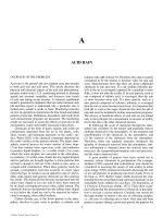
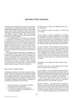
The relative shearing force required to deform a fluid
gives a measure of the viscosity of the fluid. An increase
in temperature causes a decrease in viscosity of a liquid

and vice versa. Consider the space between two parallel
plate remains at rest while the upper plate moves with
velocity V under an applied force. The velocity of the fluid
particles will range from V at the top boundary to zero at
the bottom as they will assume the same velocity as the
boundary in which they are in contact. Experiments have
demonstrated that the shear stress, t, is directly propor-
tional to the rate of deformation, d u /d y. Mathematically,
this can be written as:

t ϭ
d
d
u
y⋅
(2)
Equation (2) is known as Newton’s equation of viscosity.
The constant of proportionality, µ, in newton-second per
square meter (N-s/m
2
), is termed the coefficient of viscosity,
the dynamic viscosity or the absolute viscosity.
The kinematic viscosity, v, is defined as the ratio of the
coefficient of viscosity to the density and is expressed in

v ϭ
m
r ⋅
(3)
A more proper term for surface tension, s, would be surface

energy. Surface tension is a liquid surface phenomenon
and is caused by the relative forces of cohesion, the attrac-
tion of liquid molecules for each other, and adhesion, the
attraction of liquid molecules for the molecules of another
liquid or solid. Surface tension has the units of newtons per
meter (N/ m). When a liquid surface is in contact with a solid,
a contact angel u, greater than 90Њ results with depression of
the liquid surface if the liquid does not “wet” the tube such
as mercury and glass. If the solid boundary has a greater
attraction for a liquid molecule than the surrounding liquid
molecules, then the contact angle is less than 90ЊC and the
liquid is said to “wet” the wall leading to a capillary rise as
in the case of water and glass.
in the preceding paragraphs for a few common fluids.
PRESSURE FLOW
Friction Formulae
Darcy-Weishbach ’ s Equation The Darcy-Weishbach formula
was first proposed empirically but later found by dimensional
reasoning to have a rational basis:

h
fLV
D
f
ϭ
2
2g
(4)
in which f ϭ friction factor, L ϭ pipe length, V ϭ mean
velocity, D ϭ diameter, h ϭ head loss, g ϭ acceleration due

to gravity.
Equation (4) was derived for circulation sections flowing
full and the equation itself is dimensionally homogeneous. It
can be extended to other cross-sections provided these shapes
are not too different from circular; in this case, the equation
has to be transformed by using the hydraulic radius, R, instead
of the diameter, D:

h
fLV
R
f
ϭ
2
8g
,
(5)
C023_003_r03.indd 1275C023_003_r03.indd 1275 11/18/2005 11:12:11 AM11/18/2005 11:12:11 AM
© 2006 by Taylor & Francis Group, LLC
Table 1 gives the values of the fluid properties discussed
plates (Figure 1) which is filled with fluid; the bottom
1276 WATER FLOW
where r ϭ D /4 for flow at full bore. The use of Darcy’s
equation in the form given by Eq. (5) is sometimes extended
to open channel flow.
The determination of the friction factor, f, depends on
the flow regime, that is, whether the flow is laminar, critical,
transitional, smooth, turbulent or rough fully turbulent.
Laminar Flow Consider the mean pipe velocity, V, as
given by Hagen-Poiseuille’s equation for laminar flow:

V ϭ
g
m
SD
32
(6)
in which S ϭ energy slope.
Combining Eq. (4) with Eq. (6) and noting that S ϭ H
f
/L,
g ϭ rg, and nmրr, the friction factor is given by:

f
e
ϭ
64
R
,
(7)

where R
e
ϭ nDրg is the Reynolds number. Eq. (7) can be
used for all pipe roughness as the friction factor in lami-
nar flow is independent of the wall protuberances and is
inversely proportional to the Reynolds number. The energy
loss varies directly as the mean pipe velocity in laminar flow
which persists up to a Reynolds number of about 2000.
The velocity profile, which has a parabolic distribu-

tion, can be obtained from Hagen-Poiseuille’s equation. The
velocity, u, at any radius, r, of the pipe of diameter, D, is
given by:

u
SD
ϭϪ
g
m44
2
2
r
⎛
⎝
⎜
⎞
⎠
⎟
.
(8)
At the centre line, the velocity is a maximum:

u
SD
max
ϭ
g
m
2
16

(9)
The mean velocity is:

uu
SD
mean
/ϭϭ() .
max
2
32
2
g
m
(10)
Critical Flow From a Reynolds number of about 2000 and
extending to 4000 lies a critical zone where the flow may be
either laminar or turbulent. The flow regime is unstable and
no equation adequately describes it.
Smooth Turbulent For pipes fabricated from hydraulically
smooth materials such as copper, plexiglass and glass, the
flow is smooth turbulent for a Reynolds number exceeding
4000. The von Karman-Nikuradse smooth pipe equation is:

1
2080
10
f
Rf
e
ϭϪlog ( ) . .

(11)

Equation (11) indicates that the friction factor depends on
the fluid properties and deceases with increasing Reynolds
number.
Rough Fully Turbulent Nikuradse experimented with
pipes artificially roughened with uniform sand grains. The
results were fitted to the theory of Prandtl–Karman to give
the well known rough-pipe equation:

1
2114
10
f
Dϭϩlog ( ) . ./␧
(12)
TABLE 1
Fluid properties
Fluid
Temperature
ЊC
Mass density
kg/m
3
Specific weight
kN/m
3
Dynamic viscosity
N-s/m
3

Kinematic viscosity
m
2
/s
Surface tension
N/m
Water 0 1000 9.81 1.75 ϫ 10
Ϫ3
1.75 ϫ 10
Ϫ6
0.0756
— 5 1000 9.81 1.52 ϫ 10
Ϫ3
1.52 ϫ 10
Ϫ6
0.0754
— 10 1000 9.81 1.30 ϫ 10
Ϫ3
1.30 ϫ 10
Ϫ3
0.0742
Mercury 20 13,570 133.1 1.56 ϫ 10
Ϫ3
1.15 ϫ 10
Ϫ7
0.514
Sea water 20 1028 10.1 1.07 ϫ 10
Ϫ3
1.04ϫ 10
Ϫ6

0.073
Moving
plate
Applied
force
V
dy
u+dy
u
du
u = 0
Stationary
plate
y
FIGURE 1 Fluid shear.
C023_003_r03.indd 1276C023_003_r03.indd 1276 11/18/2005 11:12:11 AM11/18/2005 11:12:11 AM
© 2006 by Taylor & Francis Group, LLC
WATER FLOW 1277
Equation (12) states that beyond a certain Reynolds number,
when the flow is fully turbulent, the friction factor is influ-
enced only by the relative roughness,␧րD and independent of
the Reynolds number.
Transition Flow Most commercial pipe flows do not
follow either the smooth pipe or rough pipe equations.
Colebrook and White proposed a transitional flow equation
which would be asymptotic to both:

1
2
37

251
10
f
eD
Rf
e
ϭϪ ϩlog
.
.
.
/
⎛
⎝
⎜
⎞
⎠
⎟
(13)
Equation (13) approaches the smooth pipe equation for low
and the rough pipe equation for high values of the Reynolds
number respectively. Unlike Nikuradse’s ␧, which represents
the actual height of the sand grains, the ␧ of Colebrook—
White’s equation is not an actual roughness dimension but a
representative height describing the roughness projections. It is
referred to as the equivalent sand-grain diameter since the fric-
tion loss it represents is the same as the equivalent sand-grain
diameter; Table 2 gives experimentally observed values:
TABLE 2
Equivalent sand-grain diameter
Pipe material

␧ (mm)
Riveted steel 9.14
Rough concrete 3.05
Smooth concrete 0.31
Steel 0.05
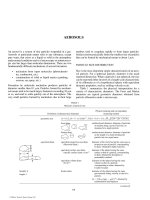
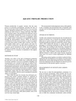
Moody Diagram (Moody, 1944.) The Moody Diagram
(Figure 2) summarises and solves graphically the four fric-
tion factor equations Eqs. (7), (11), (12), (13) as well as
delineating the zones of the various flow regimes. The line
separating transitional and fully turbulent flow is given by
Rouse’s equation:

1
200
f
R
D
e
ϭ
␧
.
(14)

Mannning ’ s Equation The Manning equation, although
originally developed for open channel flow, has often been
extended for use in pressure conduits. The equation is usu-
ally favored for rough textured material (rough concrete,
unlike rock tunnels) and cross-sections that are not circular
(rectangular, horseshoe). It is most commonly given in the
form:

v
N
RSϭ
1
23 12//
,
(15)
in which N ϭ roughness coefficient. Equation (15) can also
be transformed to:

hN
L
R
V
f
ϭ19 6
2
2
43
2
.,
/
g
(16)

S
N
AR
ϭ

Q
22
243/
.
(17)
FIGURE 2 Pipe friction factors.
Friction factor f
Critical
Smooth pipes
0.01
0.02
0.03
0.04
0.05
0.06
10
3
10
4
10
5
10
6
10
7
Relative roughness
⑀/D
turbulent
Fully
0.0001

0.004
0.001
0.002
0.004
⑀/D = 0.010
Reynolds number VD/ν
C023_003_r03.indd 1277C023_003_r03.indd 1277 11/18/2005 11:12:12 AM11/18/2005 11:12:12 AM
© 2006 by Taylor & Francis Group, LLC
1278 WATER FLOW
The dimension of the roughness coefficient, N, is frequently
taken as L
1/6
as the equation by itself is not dimensionally
homogenous. Table 3 provides values of Manning’s N for the
more widely used pipe materials.
Hazen-William ’ s Equation This equation is used mainly in
sanitary engineering.
V ϭ 0.36 CR
0.63
S
0.54
, (18)
where C ϭ roughness coefficient. Typical values of the
Hazen-William’s C is given in Table 4.
Energy Losses Due to Cross-Sectional Changes,
Bends and Valves
Cross-Sectional Changes
Expansion Energy loss in an expansion is principally a
form loss:

h
D
D
V
exp
,ϭϪ1
2
1
2
2
2
1
2
⎛
⎝
⎜
⎞
⎠
⎟
⎡
⎣
⎢
⎢
⎤
⎦
⎥
⎥
g
(19)
in which D ϭ diameter of the conduit, and subscripts 1 and

2 denote upstream and downstream values. From Eq. (19), if
D
2
is very large compared to D
1
, such as the discharge into a
reservoir, the entire velocity head is lost.
Contraction The contraction loss equation can be expres sed
in terms of the downstream velocity, V
2
,

as:

H
C
V
c
con
ϭϪ
1
1
2
2
2
⎛
⎝
⎜
⎞
⎠

⎟
g
.
(20)
Typical values of the coefficient of contraction, C
c
, are given
in Table 5.
Entrance Loss The head loss at the entrance of a conduit
can be compared to that of a short tube:

h
C
V
ent
ϭϪ
1
1
2
2
2
⎛
⎝
⎜
⎞
⎠
⎟
g
(21)

hK
V
ent end
ϭ
2
2g
,
(22)

in which C ϭ coefficient of discharge, K ϭ entrance loss
coefficient. Typical values of C and K are given in Table 6.
Transition In gradual contractions and expansions, the
lead losses are calculated in terms of the difference of veloc-
ity heads in the upstream and downstream pipes:

Gradual contraction: hK
VV
tc te
ϭϪ
2
2
1
2
22gg
⎛
⎝
⎜
⎞
⎠
⎟

,
(23)

Gradual ex n: pansio hK
VV
tc te
ϭϪ
22
22gg
⎛
⎝
⎜
⎞
⎠
⎟
.
(24)
K
tc
values vary from 0.1 to 0.5 for gradual to sudden contrac-
tions. Values of K
tc
range from 0.03 to 0.80 for flare angles of
2Њ to 60Њ.
TABLE 4
Hazen-William’s C
Material (new) C
Cast iron 130
Welded steel 119
Riveted steel 110

Concrete 130
Wood-stave 120
Vitrified clay 110
TABLE 3
Normal values of Manning’s N
Material N
Brass 0.010
Corrugated metal 0.024
Glass 0.010
Concrete, unfinished 0.014
Vitrified clay 0.014
Steel 0.012
Cement 0.012
Brick 0.013
TABLE 5
Coefficient of contraction
A
2
/A
1
C
c
0.25 0.64
0.50 0.68
0.75 0.78
1.00 1.00
TABLE 6
Values of C and K
ent
Type of entrance C K

ent
Circular bellmouth 0.98 0.05
Square bellmouth 0.93 0.16
Fully rounded 0.95 0.10
Moderately rounded 0.89 0.25
Sharp cornered 0.82 0.50
C023_003_r03.indd 1278C023_003_r03.indd 1278 11/18/2005 11:12:13 AM11/18/2005 11:12:13 AM
© 2006 by Taylor & Francis Group, LLC
WATER FLOW 1279
Bends The effect of the presence of bends is to induce
secondary flow currents which are responsible for the addi-
tional energy dissipation:

hK
V
bb
ϭ
2
2g
.
(25)
The bend loss coefficient, K
b
, depends on the ratio of the
bend radius, r, to the pipe diameter, d, as well as the bend
angel. For a 90Њ bend and r / d ratio varying from 1 to 12,
values of K
b
range from 0.20 to 0.07.
Gates and Gate Valves The gate and gate valve loss can

be expressed as:

hK
V
gg
ϭ
2
2g
(26)
The value of the loss coefficient, K
g
, for gates depends on
a variety of factors. The value of K
g
for the case having the
bottom and sides of the jet suppressed ranges from 0.5 to 1.0.
for typical values of K
g
for gate valves see Table 7.
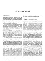
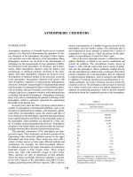
Energy-discharge Relation
In pressure conduit flow, the water is transmitted through a
closed boundary conveying structure without a free surface.
Figure 3 illustrates graphically the various forms of energy
losses which could take place within the conduit. The follow-
ing energy relation can be written:

hh h h
lf
ϭϩϩ
ent tc

(28)
in which h
end
ϭ entrance loss, h
tc
ϭ transition loss, h
f
ϭ skin
friction loss. If H denotes the total head required to produce
the discharge and h
v
represents the existing velocity head,
H ϭ h
l
ϩ h
v
. (29)
Writing Eq. (29) in terms of the velocity heads and their
respective loss coefficients,

HC
V
K
V
K
VV
f
LV
D
K

l
v
ϭϭ ϩ
ϩϩ
2
2
2
2
2
2
2
gggg
g
ent
1
2
tc
2
2
1
2
22

2
−
⎛
⎝
⎜
⎞
⎠

⎟
⎡
⎣
⎢
⎢
VV
2
2
2g
⎤
⎦
⎥
,
(30)
where K
v
ϭ combined velocity head and exit loss coefficient.
By the continuity equation:

AV AV
11 22
ϭ
(31)
and

VA
A
V
1
2

2
2
1
2
2
22gg
ϭ .

Equation (30) could be expressed as,

HC
V
V
K
A
A
K
A
A
fL
gD
K
l
v
ϭ
ϭϩϩϩ
2
2
2
2

2
1
2
2
2
1
2
2
2
2
1
2
g
g
ent tc
⎛
⎝
⎜
⎞
⎠
⎟
−
⎛
⎝
⎜
⎞
⎠
⎟
⎡⎡
⎣

⎢
⎢
⎤
⎦
⎥
⎥
(32)
in which

CK
A
A
K
A
A
fL
D
K
ltc v
ϭϩϩϩ
ent
2
1
2
2
2
1
2
2
1

2
⎛
⎝
⎜
⎞
⎠
⎟
−
⎛
⎝
⎜
⎞
⎠
⎟
⎡
⎣
⎢
⎢
⎤
⎦
⎥
⎥
g

(33)

V
C
H
l

2
12
1
2ϭ
/
g
(34)


QAV
A
C
gH
CA H
ϭϭ
ϭ
22
2
1
12
2
2
2
/
g ,
(35)
TABLE 7
K
g
for gate values

Fully open 0.2
3
4

open
1.3
1
2

open
5.5
1
4

open
24.0
Exit Loss In general the entire velocity head is lost at
exit and the exit loss coefficient, K
e
is unity in the equation:

hK
V
ee
ϭ
2
2g
.
(27)
h

ent
h
tc
TEL
Transition
H
h
l
–V
2
/2g
h
f
h
v
p/y
FIGURE 3 Energy relations.
C023_003_r03.indd 1279C023_003_r03.indd 1279 11/18/2005 11:12:13 AM11/18/2005 11:12:13 AM
© 2006 by Taylor & Francis Group, LLC
1280 WATER FLOW
in which

CC
l
ϭ1
12
/
/

is the discharge coefficient. Equation (35)

can be readily extended to multiple conduits in parallel.
Pipe Networks
Introduction The Hardy Cross method is most suitably
adapted to the resolution of pipe networks. The statement of
the problem resolves itself into:
1) the method of balancing heads is directly appli-
cable if the discharges at inlets and outlets are
known,
2) the method of balancing flows is very suitable if
the heads at inlets and outlets are known.
It is assumed that:
a) sizes, lengths and roughness of pipes in the system
are given,
b) law governing friction loss and flow for each pipe
is known,
c) equations for losses in junctions, bends, and other
minor losses are known. These relations are most
conveniently expressed in terms of equivalent
lengths of pipes.
The objectives of the analysis are:
a) to determine the flow distribution in the individual
pipes of the network,
b) to compute the pressure elevation heads at the
junctions.
In applying the Hardy Cross Method, two sets of condi-
tions have to be satisfied:
a) the total change in pressure head along any closed
circuit is zero:

H ϭ 0,

∑
(36)
b) the total discharge arriving at any nodal point
equals the total flow leaving it:

Qϭ 0.
∑
(37)
For the pressure head change in any closed path, the clock-
wise positive sign convention is used.
For the discharge continuity requirement at a nodal point,
the inward flow positive sign convention is adopted.
The friction head loss equation is used in the form:

HrQϭ
2
.
(38)
Using Darcy’s formula:

H
fLV
D
fL
D
Qϭϭ
2
25
2
2

8
ggp
⎛
⎝
⎜
⎞
⎠
⎟

and

r
fL
D
ϭ
8
25
gp
.

Method of Balancing Heads Based on the condition required
by Eq. (36), the following equations for any closed pipe loop
results (Figure 4):

HrQQ
∑∑
ϭϩϭ(),
0
2
0⌬ (39)

where Q
0
ϭ assumed flow in the circuit for any one pipe,
⌬ Q ϭ required flow correction. Expanding Eq. (39) and
approximating by retaining only the first two terms, the flow
correction ⌬ Q, can be expressed as:

⌬Q
rQ
rQ
ϭ
Ϫ
0
2
0
2
∑
∑
.
(40)
Method of Balancing Flows Utilising the continuity require-
ment at a pipe junction as given by Eq. (37), the head
correction, ⌬ H, at anodal point is given by the equation:

⌬H
H
r
H
H
r

ϭ
⎛
⎝
⎜
⎞
⎠
⎟
⎛
⎝
⎜
⎞
⎠
⎟
∑
∑
12
12
1
2
/
/
.
(41)
In both Eq. (40) and (41), the proper sign conventions must
be used in the numerators.
OPEN CHANNEL FLOW
Introduction
Open channel flow refers to that class of water discharge in
which the water flows with a free surface. The stream flow
is said to be steady if the discharge does not vary with time.

If the discharge is time dependent, the water flow is termed
unsteady. Uniform flow refers to the case in which the mean
velocities at any cross-section of the stream are identical; if
these mean velocities vary from one cross-section to another,
the flow is considered non-uniform. Steady uniform flow
requires the conveyance section of the stream channel to
be prismatic. Where the water surface profile is controlled
+
+
Q
Q
FIGURE 4 Pipe network.
C023_003_r03.indd 1280C023_003_r03.indd 1280 11/18/2005 11:12:13 AM11/18/2005 11:12:13 AM
© 2006 by Taylor & Francis Group, LLC
WATER FLOW 1281
principally by channel friction, this phenomenon is known as
gradually varied flow. For the type of flow in which the water
surface changes substantially within a very short channel
length due to a sudden variation in bed slope or cross-section,
this category is referred to as rapidly varied flow.
Open channels fabricated from concrete are often rect-
angular or trapezoidal in shape. Canals excavated in erodible
material have trapezoidal cross-sections. Although sewer
pipes are closed sections, they are still considered as open
channels so long as they are not flowing full; these cross-
sections are usually circular.
Channel Friction Equation
The most widely used open channel friction formula is the
Manning equation as mentioned earlier in pressure flow:

Q
N
AR Sϭ
1
23 12//
(42)

S
N
AR
ϭ
Q
22
243/
.
(17)
Manning’s equation in hydraulic engineering is used for fully
turbulent flow and, as such, the values of Manning’s N apply
to this flow regime.
In a natural tortuous stream channel, the mean value
of Manning’s N can be obtained from the following
considerations:
1) estimate an equivalent basic N
s


,

for a straight chan-
nel of that material,

2) select modifying values of N
m
for non-uniform
roughness, irregularity, variation in shape of cross-
section, vegetation, and meandering,
3) sum the basic, N
s
together with the modifying
values to obtain the total mean N.
Normal values of Manning’s N for straight channels
and various modifying values are given in Table 8. The total
mean N value for the channel is obtained from the relation:

NN N
sm
ϭϩ .
∑
(43)
Energy Principles
In deriving the energy relationships for open channel flow,
the following assumptions are normally used:
1) a uniform velocity distribution over the cross-
section is assumed, that is, the velocity coefficient,
a, in the velocity head term, aV
2
/2 g, is taken as
unity. In practice, the value of ␣ depends on the
shape of the stream channel and has an average
value of about 1.02 which makes this assumption
sufficiently valid.

2) streamlines are essentially parallel,
3) channel slopes are small.
Consider the water particle of mass, m, and of weight, W
(Figure 5). The elevation and pressure energies of the parti-
cle are Wh
1
; and Wh
2
respectively. Thus, the potential energy
of the water particles is, W ( h
1
ϩ h
2
) and is independent of its
elevation over the flow cross-section. As the kinetic energy
is WV
2
/2 g the total energy of the water particles, e is:

eWhh
V
ϭϩϩ
12
2
2g
⎛
⎝
⎜
⎞
⎠

⎟
.
(44)

ZDh hϩϭϩ
12
(45)
and noting that the total flow passing the cross-section is gQ
the total energy of the water passing the cross-section per
second, E
t
is given by:

EQZD
V
t
ϭϩϩg
2
2g
⎛
⎝
⎜
⎞
⎠
⎟
.
(46)
TABLE 8
Values of Manning’s N
Basic N

S
for straight channels
Type of channel
N
s
Earth 0.010
Sand 0.012
Fine gravel 0.014
Rock 0.015
Coarse gravel 0.028
Cobbles and boulders 0.040
Modifying values of N
m
N
s
Irregularity 0.005 to 0.020
Changes in shape 0.005 to 0.020
Vegetation 0.005 to 0.100
Meander
0.10 N
s
to 0.40 N
s
V
1/2g
2
(1)
(2)
V
1

D
1
D
h
2
Z
1
Z
L
TEL
h
f
V
2
/2g
2
h
1
i
V
2
D
2
Z
2
FIGURE 5 Energy principles.
C023_003_r03.indd 1281C023_003_r03.indd 1281 11/18/2005 11:12:14 AM11/18/2005 11:12:14 AM
© 2006 by Taylor & Francis Group, LLC
1282 WATER FLOW
Thus, the energy per unit weight of water passing the cross-

section per second, H is:

HZD
V
ϩϩϩ
2
2g
.
(47)
The term, z ϩ D ϩ V
2
ր2g is known as the total head or total
energy level (TEL); the latter name is used here. The slope
of the total energy level line is the energy gradient or friction
slope and gives the rate of energy dissipation in the flow.
The energies at Sections 1 and 2 are related by the
expression:

zD
V
ZD
V
QN
AR
11
1
2
22
2
2

22
24
22
ϩϩ ϭϩϩ ϩ
gg
/
(48)

in which the Manning equation is used to calculate the fric-
tion slope and the mean values for the flow area, A, and the
hydraulic radius, R, are to be used.
Flow Regimes
Critical Flow The specific energy, E, is defined as the total
head referred to the channel bottom (Figure 6):

ED
Q
A
ϭϩ
1
2
2g
. (49)
Differentiating Eq. (47) with respect to D and equating the
derivative to zero to obtain its minimum value,

d
d
d
d

E
D
Q
A
A
D
ϭϪ ϭ10
2
3
g
. (50)
Noting that d A ϭ T d D, Eq. (50) becomes:

QA
T
23
g
ϭ .
(51)
Equation (51) is the fundamental equation for critical flow
and is applicable to all shapes of cross-sections.
If the mean depth of the flow section is defined as
D
m
ϭ A/T, substitution of this relation into Eq. (49) would
give the significant expressions:

VD
cm
2

22g
ϭ
(52)
and

V
D
c
m
g
ϭ1.
(53)

At critical flow, Eq. (52) demonstrates that the velocity head
equals one-half the mean depth and Eq. (53) indicates that
the Froude number equals unity.
Specific Energy Diagram for Rectangular Channel For a
rectangular channel, Q ϭ qB in which q ϭ discharge per unit
width, B ϭ channel width, and Eq. (49) becomes,

ED
q
D
ϭϩ
2
2
2g
.
(54)
A plot of Eq. (54) for any given constant unit discharge gives

Figure 7, which is known as the specific energy diagram. The
TEL
E
D
T
D
dD
dA
V
2
/2g
FIGURE 6 Derivation of critical flow.
45° line
E = D
Flow depth, D
Critical line
q
1
q
2
Supercritical
E
c
= D
c
3
2
Subcritical
FIGURE 7 Specific energy diagram.
C023_003_r03.indd 1282C023_003_r03.indd 1282 11/18/2005 11:12:14 AM11/18/2005 11:12:14 AM

© 2006 by Taylor & Francis Group, LLC
WATER FLOW 1283
following flow regimes could be defined with reference to the
specific energy diagram.
Subcritical flow denotes tranquil flow in which the
Froude number and the mean velocity are less than unity and
the celerity of the gravity wave respectively.
Critical flow represents the discharge phenomenon
where: (1) for a constant specific energy, the discharge is a
maximum; (2) the specific energy is a minimum for a con-
stant discharge; (3) the critical velocity equals the celerity of
a small gravity wave; (4) the Froude number equals unity;
(5) the critical depth is also the depth of minimum pressure-
momentum force.
Supercritical flow which is also known as shooting
or rapid flow, is that state of water flow where the Froude
number and mean velocity exceed unity and the speed of
transmission of a surface wave respectively.
Based on the equations developed earlier for critical
flow, particular formulae can be derived for a rectangular
section:

D
q
c
c
ϭ
g
⎛
⎝

⎜
⎞
⎠
⎟
13/
(55
)

DE
cc
ϭ
2
3
()
(56)


D
V
c
c
ϭ
2
g
(57)


V
D
c

c
g
ϭ1.
(58)
Flow Transition The concept of the normal depth is an impor-
tant parameter in the study of flow transition. For a given
channel and any fixed discharge, uniform flow will occur at
one unique depth. It is the depth attained in a long channel
when the component of gravity force is just balanced by the
frictional resistance of the channel.
When the normal and critical depth are equal, the flow
is critical and the bed and energy slopes are the same.
The channel bed then has a critical slope. The bed slope
is termed mild when the normal depth exceeds the critical
depth; the bed slope is then less than the critical energy
slope and the flow regime is subcritical. When the normal
depth lies below the critical depth and, hence, the bed slope
is greater than the critical energy slope, the channel slope
is considered to be steep and the supercritical flow regime
prevails.
When water makes a transition from a channel with a
mild slope to another with a steep slope, or vice versa, the
flow passes through the critical depth close to the junction
of the two channels. The section in which the water depth is
critical defines a channel control. The weir acts as a control
when water flows over it as critical depth is attained there.
Hydraulic Jump A hydraulic jump occurs when supercritical
flow makes a transition to subcritical flow. A common occur-
rence of a hydraulic jump takes place at the base of a chute
spillway. Figure 8 shows the energy momentum and depth

relations for a hydraulic jump and also defines the symbols
to be used.
In developing the equations for the hydraulic jump, the
following assumptions are used:
1) the bed slope is considered small and neglected,
2) frictional resistance along the bed and sides of the
channel are omitted.
Consider the control volume between Sections (1) and (2).
Applying the impulse-momentum principle:

FF QVV
12 21
Ϫϭ Ϫ
g
g
()
(59)
or

FQVFQV
1122
ϩϭϩ
gg
gg
(60)
in which F
1
and F
1
denote the hydrostatic forces at sections 1

and 2 respectively. The term (F ϩ g/gQV) is given the name
pressure-momentum force. Let A ϭ flow area, y
–
ϭ distance
of centroid of flow area from surface; then they hydrostatic
force ϭ gAy
–
and Eq. (60) can be written as:

Ay
Q
A
Ay
Q
A
11
2
1
21
2
2
ϩϭ ϩ
gg
.
(61)

Equation (60) states the condition for the formation of a
hydraulic jump and suggests a graphical solution. A plot of
Eq. (60) for any fixed discharge is shown in Figure 8. For any
given up-stream supercritical water depth, which is usually

known such as at the toe of a spillway, the subcritical hydraulic
jump depth or sequent depth can be obtained from the graph.
For a rectangular cross-section channel and utilising the
continuity relation:

QVA VAϭϭ
11 2 2
.
(62)
D
S.E.
P.M.F.
D
D
TEL
E
j
V
2
/2g
2
F
V
1
/2g
2
D
c
F
2

(1)
(2)
E
P.M.F.
FLOW
FIGURE 8 Hydraulic jump relations.
C023_003_r03.indd 1283C023_003_r03.indd 1283 11/18/2005 11:12:14 AM11/18/2005 11:12:14 AM
© 2006 by Taylor & Francis Group, LLC
1284 WATER FLOW
Equation (6) can be written as:

D
D
F
2
1
1
2
1
2
18 1ϭϩϪ(),
(63)

where

FV D
11 1
ϭ /( )g

is the upstream Froude number.

The energy loss E
j
across the hydraulic jump on a
horizontal floor can be obtained by coming Eqs. (61), (62)
and the energy equation:

D
V
D
V
E
j1
1
2
2
2
2
22
ϩϭϩϩ
gg
(64)
to give:

E
DD
DD
j
ϭ
Ϫ()
.

21
3
12
4
(65)
The head loss E
j
is graphically shown in the specific energy
Surface Water Profiles
Non-uniform Differential Equation Using the notation given
in Figure 9, the energy relations can be expressed as:

iL D
V
SL D D
VV
ϩϩ ϭ ϩ ϩ ϩ ϩ
222
222ggg
dd d()
⎛
⎝
⎜
⎞
⎠
⎟
(66)


d

d/
L
DV
iS
ϭ
ϩ
Ϫ
(
()
2
2g)
(67)

d
d
E
L
iSϭϪ().
(68)
For a finite length, ⌬ L, Eq. (67) becomes:

⌬LLL
DV DV
iQNAR
ϭϪ
ϭ
ϩϪϩ
Ϫ
()
()()

,
21
11
2
22
2
22 243
22//
/
/
gg
⎛
⎝
⎜
⎞
⎠
⎟
(69)
where the Manning equation is used to calculate the energy
slope. Flow computation must start at a control section
where all the flow parameters are known. The calculation
proceeds upstream for subcritical and downstream for super-
critical flow. In Eq. (69), the solution of the reach length,
⌬ L, is direct if the immediately upstream depth, D
2
, is given
a value. If ⌬ L is given a value, D
2
has to be solved by trial.
This method of computing surface water profiles is suitable

for regular channels.
Classification of Flow Profiles Twelve distinct types of
non- uniform profiles have been systematically classified
1) Firstly, the curves are identified according to bed
slopes as mild (M), steep (S), horizontal (H), criti-
cal (C) and adverse (A).
2) Secondly, numbers are assigned to flow regions.
The numerical 1 refers to actual flow depths
exceeding both critical ( D
c
) and normal ( D ) depths.
For flow depths less than both critical and normal,
the number 3 is affixed to it. The numeral 2 is for
depths intermediate between critical and normal.
Water Profiles in Irregular Channels The river channel has
conveying overbank flow. Let Q ϭ total flow, Q
c
ϭ central
channel discharge, Q
l
ϭ left overbank flow,
Q
r
ϭ right overbank flow. The continuity condition
requires that:

QQ QQ
clr
ϭϩϩ, (70)
By Manning’s Equation:

Q
N
AR S
N
AR S
N
AR S
c
cc
l
l
r
rr
ϭϩϩ
111
23 12 23 12 23 12// // //
.

(71)

The energy slope, S, has been taken as the same for Q
c
,
Q
l
, Q
r
; this assumption seemed to be justified in practice.
Due to different channel roughness, vegetative and other

obstructions, Manning’s N for the three flow panels would
(1)
(2)
TEL
S
i
dL
idL
D
(D + dD)
V
2
2g
+ d (
V
2
2g
)
S dL
V
2
2g
FIGURE 9 Non-uniform flow derivation.
C023_003_r03.indd 1284C023_003_r03.indd 1284 11/18/2005 11:12:14 AM11/18/2005 11:12:14 AM
© 2006 by Taylor & Francis Group, LLC
(Figure 10).
and flow diagrams (Figure 8).
to be divided into panels (Figure 11) with the side panels
WATER FLOW 1285
not have the same values. As the energy gradient, S, is

common to the panels in Eq. (71), water level versus energy
slope curves can be plotted for any selected discharge for
water level computations. The energy equation for the step
method of surface profile calculation can conveniently be
written in the form:

WL
Q
A
WL
Q
A
SL
2
2
2
2
1
2
1
2
12
1
2
1
2
ϩϭϩϩ
gg
,
.

(72)

If in practice, the change in kinetic head,

()QAQ A
2
2
22
1
2
22//ggϪ

is small and could be removed from Eq. (72), this would
greatly simplify the work. In determining the wetted perim-
eter for the calculation of the hydraulic radius, only the
water-channel contact lines are relevant and the water-water
contact lines between panels are excluded.
FLOW IN ERODIBLE CHANNELS
Introduction
Flow in erodible channels can be divided into two types,
namely, canal and river flows. Blench describes canal flow
as possessing there degrees of freedom due to its ability to
adjust itself with respect to its flow depth, bed slope, and side
widths which are taken to be the dependent variables. River
flow, in addition to having the three degrees of freedom of
canals, has a fourth degree by virtue of its ability to meander.
It is assumed that constant maintenance of canals suppresses
the canal’s tendency to meander. The water-sediment flow is
usually regarded as the independent parameter.
In the concept of flow in mobile channels where the

transport of sediment is an integral part of the system, two
philosophies have emerged. Based on the work of Lindley
(1919), Lacey (1952), Inglis (1949), and Blench (1953, 1966)
in India and Pakistan, the regime theory has evolved. On the
other hand, the United States Bureau of Reclamation under
the direction of Lane (1952, 1953) developed the tractive
force method.
Regime Theory for Canals
The regime theory postulates that for given water-sediment
flow and bed material, there exists a regime channel which
determines uniquely the flow area, cross-sectional shape and
bed slope. The regime channel is considered a stable chan-
nel which on the average will neither silt nor scour. The flow
occupying the regime channel is the dominant discharge and
it is also variously referred to as the formative, regime, or
bank-full discharge.
Lacey ’ s Equations Based on extensive flow observations
of the canals in India, Lacey (1952) proposed a set of for-
mulae for alluvial channels with sandy mobile beds with the
discharge ranging from 25 cfs to 2500 cfs, the bed material
size varying from 0.2 mm to 0.6 mm and with the quantity
of solids conveyed being less than 50 ppm:
Wetted perimeter:
PQϭ267
12
.
/
(73)
Flow area:
A

Q
f
ϭ
125
56
13
.
/
/

(74)
Bed slope:
S
f
Q
ϭ
0 0054
53
16
.
/
/
(75)
Silt factor:
fdϭ8
inch
1/2
.
(76)
From the above equations, the following two equations can

be derived:
Mean velocity:

VQ
r
ϭ 0 895
16 16
.
//

M1
M2
M3
Mild slope
Steep slope
C1
C3
Critical slope
Legend Normal depth
Critical depth
H2
H3
Adverse slope
A3
A2
S1
S2
S3
FIGURE 10 Surface water profiles.
Left

panel
Center
panel
Right
panel
FIGURE 11 River channel division.
C023_003_r03.indd 1285C023_003_r03.indd 1285 11/18/2005 11:12:15 AM11/18/2005 11:12:15 AM
© 2006 by Taylor & Francis Group, LLC
1286 WATER FLOW

Flow depth:
D
Q
f
ϭ
0 473
13
13
.
.
/
/

(77)
Blench ’ s Equations Blench (1953, 1966), using the concept
that canals possessing three degrees of freedom must, there-
fore, have three basic equations to describe their motion,
presented the stream equations for small bed load as:

VD F

b
2
ϭ
(78)


V
B
F
s
2
ϭ
(79)


V
DS
VB
2
14
363
g
ϭ .( )./
/
v
(80)

In Eq. 78, F
b
is bed factor and the equation itself expresses

the statement that channels with similar water-sediment
flows tend towards the same Froude number in relation to a
suitable depth. Equation (79) describes the scouring action
on the hydraulically smooth sides and defines the side Factor,
F
s
. The dissipation of energy per unit mass of water per unit
time in the channel is given by Eq. (80) in which S is the
energy gradient.
For appreciable bed load, Eq. (80) becomes:

V
DS
CVB
2
14
363 1
233g
ϭϩ.,
⎛
⎝
⎜
⎞
⎠
⎟
⎛
⎝
⎜
⎞
⎠

⎟
v
/
(81)

where C is the bed load charge in parts per hundred thousand
by weight of fluid discharge.
The bed factor, F
b
, for sand of subcritical flow is given
by the empirical equations:

FF C
bb
ϭϩ
0
1012(.)
(82)

Fd
bmm0
19ϭ .
(83)
in which F
b0
ϭ zero bed factor and is the value of F
b
when C
tends to zero, d
mm

ϭ median bed material size by weight in
millimeter. As a guide to the value of the side factor, F
s
, the
following table has been suggested by Blench (1966).
Tractive Force Method for Canals
Unit Tractive Force The stability of an erodible chan-
nel depends on (a) the resistance of the material lining the
bottom and sides against the erosive force of the stream and
(b) the ability of the stream to transport the sediment load
without giving rise to significant deposition.
The shear or drag force exerted by the water on the bed
and sides of the channel is termed the tractive force. The
average unit tractive force, t, in uniform flow is the compo-
nent of the gravity force acting on the water parallel to the
channel bottom per unit area, thus:

tgϭ RS. (84)

For wide channels, the flow depth can replace the hydraulic
radius:

tgϭ DS. (85)

The distribution of tractive force has been investigated by
the United States Bureau of Reclamation (Lane, 1952; 1953,
Olsen and Florey, 1951, 1952). The maximum values of the
unit tractive force for the bottom and sides of rectangular
and trapezoidal cross-sections are given in Figure 12.
Tractive Force Ratio A soil particle of effective area, A

e
,
resting on the side of a channel is acted on by the tractive
TABLE 9
Values of the bed factor
Material (F
s
)
max
Remarks
Very sandy loam banks 0.1
Erosion if Ͼ (F
s
)
max
Silty clay loam 0.2
Erosion if Ͼ (F
s
)
max
Very cohesive banks 0.3
Erosion if Ͼ (F
s
)
max
Trapezoidal
bottom
SS 2:1 and 1.5:1
SS 2:1, sides
SS 1.5:1, sides

SS 0:1, sides
Rectangular
SS 0:1, bottom
Width/depth ratio
Maximum unit tractive force Ϭ γDS
0
0
0.2
0.4
0.6
0.8
1.0
24
6
8
FIGURE 12 Maximum tractive force.
C023_003_r03.indd 1286C023_003_r03.indd 1286 11/18/2005 11:12:15 AM11/18/2005 11:12:15 AM
© 2006 by Taylor & Francis Group, LLC
WATER FLOW 1287
force, A
e
t
s
, in the direction of the flow and the gravity force
component, W
s
sin w which attempts to cause the particle to
roll down the side slope, where t
s
ϭ unit tractive force on the

side of the channel, W
s
ϭ submerged weight of the particle,
w ϭ angle of the channel side. The resultant of these two
forces, F, is:

FW A
scs
ϭϩ(sin ).
/22 2212
wt
(86)
The motion of the article is resisted by its frictional force ( R ):

RW
s
ϭ cos tan ,wu
(87)

where tan u is the coefficient of friction and u is the angle of
repose of the material.
Equating Eq. (86) and (87) for the condition of impend-
ing motion and solving for t
s
:

twu
w
u
s

r
e
W
A
ϭϪcos tan
tan
tan
.1
2
2
⎛
⎝
⎜
⎞
⎠
⎟
(88)

A similar equation can be written for the case of a particle on
a level bed when motion is impending, thus:

t
l
r
e
W
A
qϭ tan ,
(89)
where t

l
denotes the unit tractive force on the level bed.
The tractive force ratio, K, is defined as,

t
s
/t
l
is obtained
by dividing Eq. (87) to Eq. (88) and simplifying:

K ϭϪ(sin sin).1
2212
wu/
/
(90)

From Eq. (89) it can be seen that the tractive force ratio,
K is a function of the side slope and angle of repose of the
material only.
Critical Tractive Force The permissible tractive force is
the maximum unit tractive force that will not cause signifi-
cant scour of the material lining the channel bed on a level
surface. It is often found from laboratory observations and
is known as the critical tractive force. It is influenced by the
amount of organic matter and fine suspended sediment in
the water. The effect of the fine sediment is to increase the
allowable critical tractive force. Figure 13 shows curves of
permissible tractive forces as recommended by the United
States Bureau of Reclamation.

River Engineering
In river flows, a greater number and range of factors have
to be considered in addition to those parameters used in the
analysis of canals. These variables include bigger size bed
materials, large suspended and bed sediment loads, unsteady
and a wide variation of flood flows, meandering and braid-
ing, large changes in stream channel cross-sections, obstruc-
tions to flow, and other factors involved. An analysis of river
engineering is, therefore, beyond the scope of this chapter.
Readers are recommended to consult the works of Blench
(1966), Shen (1971, 1972), Inglis (1949) and Leopold,
Wolman and Miller (1964). More specialized treatment of
sediment transport, bedforms and stream geometry can be
found in the publications of Einstein (1972), Leopold and
Maddock (1953), Richardson and Simons (1967), Yalin
(1971), Kennedy (1963), Christensen (1972), and Ackers
(1964). Standard texts which cover the subject more formally
include those of Graf (1971), Henderson (1966), Raudkivi
(1967) and Leliavsky (1955).
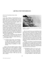
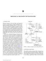
FLOW WITH AN ICE COVER
A river flowing with an ice cover has, in addition to the bed
and side frictional forces, the shear resistance imposed by
a buoyant boundary represented by the floating ice cover.
Chee and Haggag (1984) have developed equations con-
cerning floating boundary stream flow which are repro-
duced here. The essential concepts and assumptions are first
discussed.
A channel with a buoyant cover can be divided into two
(1) is influenced by the bed and sides while subsection (2) is
controlled by the cover. The two subsections are divided by

a separation surface which represents the locus of no shear
and maximum velocity. The equations of energy, continuity,
Coarse non-
cohesive
material
25% larger
Large
amount
of fine
sediment
Small amount
of fine
sediment
Clear
water
Mean diameter, mm
Critical tractive force, 1bs./ft
2
1.0
1.0
0.1
0.1
0.01
10
100
FIGURE 13 Critical tractive force for canals.
C023_003_r03.indd 1287C023_003_r03.indd 1287 11/18/2005 11:12:15 AM11/18/2005 11:12:15 AM
© 2006 by Taylor & Francis Group, LLC
subsections as shown in Figure 14. The flow in subsection
1288 WATER FLOW

and momentum are applicable to each subsection individu-
ally as well as to the entire channel cross-section.
Composite Roughness Equation
The Reynolds form of the Navier-Stokes equation was used
to develop the shear distribution and the velocity profile
was obtained using the Prandtl-von Karman mixing length
theory. In addition, a channel momentum equation and the
flow resistance formula of Manning were utilised to derive
the relationship for the division surface separating the two
flow subsections as

(. )
()
()066
1
1
1
16
12
12
12
23
16
R
NNN
q
/
/
/
/

/
/g
ϭ
Ϫ
ϩϪ
l
l
aal
−
[]
(91)

in which R ϭ hydraulic radius of entire channel, N
1
, N
2
ϭ
Manning’s roughness for the bed and cover respectively, g ϭ
acceleration due to gravity, l ϭ R
1
/ R
2
is hydraulic radius
ratio of the bed subsection to the cover subsection, a ϭ P
1
/ P
is the wetted perimeter ratio of the entire channel to the bed
subsection. The division surface is found by solving for l
using Eq. (91).
The complete roughness, N, of an ice-covered channel

is given by

N
N
N
N
1
53
1
2
53
11 1ϭϩϪ ϩϪ
Ϫ
() () .al a a l
[]
⎡
⎣
⎢
⎤
⎦
⎥
/
/
(92)

REFERENCES
1. Ackers, P., Experiments on small streams in alluvium, proceedings,
American Society of Civil Engineers Journal, Hydraulics Division, 90,
no. HY4, pp. 1–37, July 1964.
2. Albertson, M.L., J.R. Barton, and D.B. Simons, Fluid Mechanics for

Engineers, Prentice-Hall, Inc., Englewood Cliffs, NJ, 1961.
3. Allen, J. and S.P. Chee, The resistance to the flow of water round a
smooth circular bend in an open channel proceedings, Institution of
Civil Engineers, London, 23, pp. 423–424, November 1962.
4. Blench, T., Regime theory equations applied to a tidal river estuary,
proceedings, Minnesota International Hydraulics Convention I.A.H.R.
IAHR and ASCE Joint Meeting, pp. 77–83, September 1953.
5. Blench, T., Mobile-bed fluviology, University of Alberta, 1966.
6. Chee, S.P. and M.R.I. Haggag, Flow resistance of ice-covered streams,
Canadian Journal of Civil Engineering, Vol. II, No. 4, pp. 815–823,
December 1984.
7. Chow, Ven Te, Open-Channel Hydraulics, McGraw-Hill Book Com-
pany, Inc., New York, 1959.
8. Christensen, B.A., Incipient motion on cohesionless banks, Chapter 4
in Shen, Hsieh Wen, Sedimentation, Colorado, 1972.
9. Einstein, H.A., The bed load function for sediment transportation in
open channel flows, technical bulletin No. 1026, US Department of
Agriculture, Soil Conservation Service, September 1950. Also reprinted
in Appendix B in Shen, Hsieh Wen, Sedimentation, Colorado, 1972.
10. Graf, W.H., Hydraulics of Sediment Transport, McGraw-Hill Book
Company, New York, 1971.
11. Henderson, F.M., Open Channel Flow, The Macmillan Company,
New York, 1966.
12. Inglis, C.C., The behavior and control of river and canals, research
publication No. 13, Central Waterpower Irrigation and Navigation
Research Staton, Poona, 1949.
13. Kennedy, J.F., The mechanics of dunes and antidunes in erodible bed
channels, J. Fluid Mechanics, 16, part 4, 1963.
14. King, H.W., Handbook of Hydraulics, McGraw-Hill Book Company,
Inc., New York, 1954.

15. Lacey, G., Flow in alluvial channels with sandy mobile beds, Proceed-
ings, Institution of Civil Engineers, London Vol. 9, pp. 145–164, 1952.
16. Lane, E.W., Progress report on studies on the design of channels by
the Bureau of Reclamation, Proceedings, American Society of Civil
Engineers, Irrigation and Drainage Division, Vol. 79, pp. 280-1–280-31,
September 1953.
17. Lane, E.W., Progress report on results on design of stable channels, US
Bureau of Reclamation, Hydraulic Laboratory Report No. Hyd-352,
June 1952.
18. Leliavsky, Serge, An Introduction to Fluvial Hydraulics, Constable and
Co. Ltd., London, 1955.
19. Leopold, L.B. and T. Maddock, Jr., The hydraulic geometry of stream
channels and some physiographic implications, US Geological Survey,
Professional paper 252, 1953.
20. Leopold, L.B., M.G. Wolman, and J.P. Miller, Fluvial Process in Geo-
morphology, W.H. Freeman and San Francisco, 1964.
21. Lindley, E.S., Regime channels, Minutes or Proceedings, Punjab Engi-
neering Congress, Lahore, India, Vol. 7, pp. 63–74, 1919.
22. Moody, L.F., Friction factors for pipe flow, Trans. ASME., 66, No. 8,
1944.
23. Morris, H.M., Applied Hydraulics in Engineering, The Ronald Press
Company, New York, 1963.
24. Olsen, O.J. and Q.L. Florey (compilers), Stable Channel Profiles,
Hydraulic Laboratory Report No. Hyd-325, US Bureau of Reclamation,
1951.
25. Olsen, O.J. and Q.L. Florey (compilers), Sedimentation studies in open
channels: boundary shear and velocity distribution by membrane anal-
ogy, analytical and finite difference methods, US Bureau of Reclama-
tion, Laboratory Report No. Sp-34, 1952.
26. Raudkivi, A.J., Loose Boundary Hydraulics, Pergamon Press, Oxford,

1967.
27. Richardson, E.V. and D.B. Simons, Resistance to flow in sand chan-
nels, Twelfth Congress, IAHR, 1, pp. 141–150, 1967.
28. Rouse, H., editor, Engineering Hydraulics, John Wiley and Sons, Inc.,
New York, 1950.
29. Shen, Hsieh Wen, Editor, River Mechanics, I and II, Colorado, 1971.
30. Shen, Hsieh Wen, Editor,
Sedimentation: Symposium to honour Profes-
sor H.A. Einstein, Colorado, 1972.
31. Streeter, S.L., Fluid Mechanics, McGraw-Hill Book Company,
New York, 1966.
32. United States Bureau of Reclamation, Design of small dams, US Print-
ing Office, 1961.
33. Yalin, M.S., On the formation of dunes and meanders, paper C-13, pro-
ceedings Fourteenth Congress, IAHR, 3, 1971.
S.P. CHEE
University of Windsor

FIGURE 14 Ice covered channel.
P
2
2
1
P
1
C023_003_r03.indd 1288C023_003_r03.indd 1288 11/18/2005 11:12:15 AM11/18/2005 11:12:15 AM
© 2006 by Taylor & Francis Group, LLC