1999 HVAC Applications Part 10 ppsx

1.10 1999 ASHRAE Applications Handbook (SI)
Capital and interest
Salvage value
Replacements
Operating energy
Property tax
Maintenance
Insurance
Interest deduction
Table 6 summarizes the interest and principle payments for this
example. Annual payments are the product of the initial system cost
C
s,init
and the capital recovery factor CRF(i
m
,5). Also, Equation (10)
can be used to calculate total discounted interest deduction directly.
Next, apply the capital recovery factor CRF(i
′,5) and tax rate T
inc
to
the total of the discounted interest sum.
Depreciation
Use the straight line depreciation method to calculate depreciation:
Next, discount the depreciation.
Finally, the capital recovery factor and tax are applied.
U.S. tax code recommends estimating the salvage value prior to
depreciating. Then depreciation is claimed as the difference between
the initial and salvage value, which is the way depreciation is treated in
this example. The more common practice is to initially claim zero sal-

vage value, and at the end of ownership of the item, treat any salvage
value as a capital gain.
C
sinit,
ITC–
()
CRF i
′
n
(,)
$10 000 $0–
()
0.229457 $2294.57==
C
ssalv,
PWF i
′
n
(,)CRF
i
′
n
(,)1
T
salv
–
()
$1000 0.792471
×
0.229457

×
0.5
×
$90.92==
R
k
PWF i
′
k
(,)[]
CRF i
′
n
(,)1
T
inc
–
()
k 1=
n
∑
$500 0.869741
×
0.229457
×
0.5
×
$49.89==
C
e

CRF i
′
n
(,)CRF
i
″
n
(,)⁄[]
1 T
inc
–
()
$500 0.229457 0.211247
⁄[]
0.5 $271.55==
C
sassess,
T
prop
1 T
inc
–
()
$10 000 0.40
×
0.01
×
0.5
×
$20.00==

M 1 T
inc
–
()
$100 1 0.5–
()
$50.00==
I 1 T
inc
–
()
$50 1 0.5–
()
$25.00==
T
inc
i
m
P
k 1–
PWF i
d
k
(,)[]
k 1=
n
∑
CRF i
′
n

(,) …
see Table 6=
Year D
k,SL
PWF(i
d
,k)
Discounted
Depreciation
1 $1800.00 0.909091 $1636.36
2 $1800.00 0.826446 $1487.60
3 $1800.00 0.751315 $1352.37
4 $1800.00 0.683013 $1229.42
5 $1800.00 0.620921 $1117.66
Total $6823.42
$2554.66 CRF
i
′
5(,)T
inc
$2554.66 0.229457
×
0.5
×
$293.09==
T
inc
D
kSL,
PWF i

d
k
(,)[]
CRF i
′
n
(,)…
k 1=
n
∑
D
kSL,
C
sinit,
C
ssalv,
–
()
n
⁄
$10 000 $1000–
()
5
⁄
$1800.00== =
$6823.42 CRF i
′
n
(,)
T

inc
$6823.42 0.229457
×
0.5
×
$782.84==
Table 6 Interest Deduction Summary (for Example 9)
Year
Payment
Amount,
Current $
Interest
Payment,
Current $
Principal
Payment,
Current $
Outstanding
Principal,
Current $ PWF(i
d
, k)
Discounted
Interest,
Discounted $
Discounted
Payment,
Discounted $
0 — — — 10 000.00 — — —
1 2 637.97 1 000.00 1 637.97 8 362.03 0.909091 909.09 2 398.17

2 2 637.97 836.20 1 801.77 6 560.26 0.826446 691.07 2 180.14
3 2 637.97 656.03 1 981.95 4 578.31 0.751315 492.89 1 981.95
4 2 637.97 457.83 2 180.14 2 398.17 0.683013 312.70 1 801.77
5 2 637.97 239.82 2 398.17 0 0.620921 148.91 1 637.97
_________________ ___________________ _________________ ____________________
Total — 3 189.88 10 000.00 — — 2 554.66 10 000.00
Table 7 Summary of Cash Flow (for Example 10)
1234567 89 10 11
Yea r
Cash
Outlay,
$
Net Income
Before Taxes,
$
Depreciation,
$
Net Taxable
Income,
a
$
Income Taxes
@50%, $
Net Cash
Flow,
b
$
Present Worth of Net Cash Flow
10% Rate 15% Rate 20% Rate
PWF P, $ P, $ P, $

01200000000
−120 000 1.000 −120 000 −120 000 −120 000
1 0 20 000 15 000 5 000 2 500 17 500 0.909 15 900 15 200 14 600
2 0 30 000 15 000 15 000 7 500 22 500 0.826 18 600 17 000 15 600
3 0 40 000 15 000 25 000 12 500 27 500 0.751 20 600 18 100 15 900
4 0 50 000 15 000 35 000 17 500 32 500 0.683 22 200 18 600 15 700
5 0 50 000 15 000 35 000 17 500 32 500 0.621 20 200 16 200 13 100
6 0 50 000 15 000 35 000 17 500 32 500 0.564 18 300 14 100 10 900
7 0 50 000 15 000 35 000 17 500 32 500 0.513 16 700 12 200 9 100
8 0 50 000 15 000 35 000 17 500 32 500 0.467 15 200 10 600 7 600
Total Cash Flow
27 700 2 000
− 17 500
Investment Value
147 500 122 000 102 500
a
Net taxable income = net income − depreciation.
b
Net cash flow = net income − taxes.
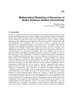
Owning and Operating Costs 1.11
Summary of terms
Cash Flow Analysis Method. The cash flow analysis method
accounts for costs and revenues on a period-by-period (e.g., year-
by-year) basis, both actual and discounted to present value. This
method is especially useful for identifying periods when net cash
flow will be negative due to intermittent large expenses.
Example 10. An eight-year study for a $120 000 investment with depreci-
ation spread equally over the assigned period. The benefits or incomes
are variable. The marginal tax rate is 50%. The rate of return on the
investment is required. Table 7 has columns showing year, cash outlays,

income, depreciation, net taxable income, taxes and net cash flow.
Solution: To evaluate the effect of interest and time, the net cash flow
must be multiplied by the single payment present worth factor. An arbi-
trary interest rate of 10% has been selected and the PWF
sgl
is obtained
by using Equation (4). Its value is listed in Table 7, column 8. Present
worth of the net cash flow is obtained by multiplying columns 7 and 8.
Column 9 is then added to obtain the total cash flow. If year 0 is
ignored, an investment value is obtained for a 10% required rate of
return.
The same procedure is used for 15% interest (column 10, but the
PWF is not shown) and for 20% interest (column 11).
Discussion. The interest at which the summation of present worth
of net cash flow is zero gives the rate of return. In this example, the
investment has a rate of return by interpolation of about 15.4%. If this
rate offers an acceptable rate of return to the investor, the proposal
should be approved; otherwise, it should be rejected.
Another approach would be to obtain an investment value at a
given rate of return. This is accomplished by adding the present worth
of the net cash flows, but not including the investment cost. In the
example, under the 10% given rate of return, $147 700 is obtained as an
investment value. This amount, when using money that costs 10%,
would be the acceptable value of the investment.
Computer Analysis
Many computer programs are available that incorporate the eco-
nomic analysis methods described above. These range from simple
macros developed for popular spreadsheet applications to more
comprehensive, menu-driven computer programs. Commonly used
examples of the latter include Building Life-Cycle Cost (BLCC),

Life Cycle Cost in Design (LCCID), and PC-ECONPACK.

BLCC was developed by the National Institute of Standards
and Technology (NIST) for the U.S. Department of Energy
(DOE). The program follows criteria established by the Federal
Energy Management Program (FEMP) and the Office of Manage-
ment and Budget (OMB). It is intended for the evaluation of
energy conservation investments in nonmilitary government
buildings; however, it is also appropriate for similar evaluations
of commercial facilities.
LCCID is an economic analysis program tailored to the needs of
the U.S. Department of Defense (DOD). Developed by the U.S.
Army Corps of Engineers and the Construction Engineering
Research Laboratory (USA-CERL), LCCID uses economic criteria
established by FEMP and OMB.
PC-Econpack, developed by the U.S. Army Corps of Engineers
for use by the DOD, uses economic criteria established by the OMB.
The program performs standardized life-cycle cost calculations
such as net present value, equivalent uniform annual cost, SIR, and
discounted payback period.
Macros developed for common spreadsheet programs generally
contain preprogrammed functions for the various life-cycle cost cal-
culations. Although typically not as sophisticated as the menu-
driven programs, the macros are easy to install and easy to learn.
Reference Equations
Table 8 lists commonly used discount formulas as addressed by
NIST. Refer to NIST Handbook 135 (Ruegg) and Table 2.3 in that
handbook for detailed discussions.
SYMBOLS
c = cooling system adjustment factor

C = total annual building HVAC maintenance cost
C
e
= annual operating cost for energy
C
s,assess
= assessed system value
C
s,init
= initial system cost
C
s,salv
= system salvage value at end of study period
C
y
= uniform annualized mechanical system owning, operating,
and maintenance costs
CRF = capital recovery factor
CRF(i,n) = capital recovery factor for interest rate i and analysis period n
CRF(i
′,n) = capital recovery factory for interest rate i′ for items other
than fuel and analysis period n
CRF(i
″,n) = capital recovery factor for fuel interest rate i″ and analysis
period n
CRF(i
m
,n) = capital recovery factor for loan or mortgage rate i
m
and anal-

ysis period n
d = distribution system adjustment factor
D
k
= depreciation during period k
Capital and interest
−$2294.57
Salvage value +$ 90.92
Replacements
−$ 49.89
Operating costs
−$ 271.55
Property tax
−$ 20.00
Maintenance
−$ 50.00
Insurance
−$ 25.00
Interest deduction +$ 293.09
Depreciation deduction +$ 782.84
Total annualized cost
−$1544.16
Table 8 Commonly Used Discount Formulas
Name Algebrac Form
a,b
Single compound-amount (SCA)
equation
Single present value (SPW)
equation
Uniform sinking-fund (USF)

equation
Uniform capital-recovery (UCR)
equation
Uniform compound-account
(UCA) equation
Uniform present-value (UPW)
equation
Modified uniform present-value
(UPW*) equation
where
A = end-of-period payment (or receipt) in a uniform series of payments
(or receipts) over n periods at d interest or discount rate
A
0
= initial value of a periodic payment (receipt) evaluated at the begin-
ning of the study period
A
t
= A
0
·(1 + e)
t
, where t = 1,…, n
d = interest or discount rate
e = price escalation rate per period
Source: NIST Handbook 135 (Ruegg).
a
Note that the USF, UCR, UCA, and UPW equations yield undefined answers when
d= 0. The correct algebraic forms for this special case would be as follows: USF
formula, A = F/N; UCR formula, A = P/N; UCA formula, F = A·n. The UPW*

equation also yields an undefined answer when e = d. In this case, P = A
0
·n.
b
The terms by which the known values are multiplied in these equations are the
formulas for the factors found in discount factor tables. Using acronyms to represent
the factor formulas, the discounting equaitons can also be written as F = P·SCA,
P=F·SPW, A = F·USF, A = P·UCR, F = UCA, P = A·UPW, and P = A
0
·UPW*.
FP1 d+
()
n
[]⋅
=
PF
1
1 d+
()
n

⋅
=
AF
d
1 d+
()
n
1–

⋅
=
AP
d 1 d+
()
n
1 d+
()
n
1–

⋅
=
FA
1 d+
()
n
1–
d

⋅
=
PA
1 d+
()
n
1–
d 1 d+
()
n

⋅
=
PA
0
1 e+
de–



1
1 e+
1 d+



n
–
⋅⋅
=
1.12 1999 ASHRAE Applications Handbook (SI)
D
k,SL
= depreciation during period k due to straight line depreciation
method
D
k,SD
= depreciation during period k due to sum-of-digits deprecia-
tion method
F = future value of a sum of money

h = heating system adjustment factor
i = compound interest rate per period
i
d
= discount rate per period
i
m
= market mortgage rate
i
′ = effective interest rate for all but fuel
i
″ = effective interest rate for fuel
I = insurance cost per period
ITC = investment tax credit
j = inflation rate per period
j
e
= fuel inflation rate per period
k = end of period(s) during which replacement(s), repair(s),
depreciation, or interest are calculated
M = maintenance cost per period
n = number of periods under analysis
P = present value of a sum of money
P
k
= outstanding principle on loan at end of period k
PMT = future equal payments
PWF = present worth factor
PWF(i
d

,k) = present worth factor for discount rate i
d
at end of period k
PWF(i
′,k) = present worth factor for effective interest rate i′ at end of
period k
PWF(i,n)
sgl
= single payment present worth factor
PWF(i,n)
ser
= present worth factor for a series of future equal payments
R
k
= net replacement, repair, or disposal costs at end of period k
T
inc
= net income tax rate
T
prop
= property tax rate
T
salv
= tax rate applicable to salvage value of system
REFERENCES
Akalin, M.T. 1978. Equipment life and maintenance cost survey. ASHRAE
Transactions 84(2):94-106.
DOE. International performances measurement and verification protocol.
Publication No. DOE/EE-0157. U.S. Department of Energy.
Dohrmann, D.R. and T. Alereza. 1986. Analysis of survey data on HVAC

maintenance costs. ASHRAE Transactions 92(2A):550-65.
Easton Consultants. 1986. Survey of residential heat pump service life and
maintenance issues. Available from American Gas Association, Arling-
ton, VA (Catalog No. S-77126).
Grant, E., W. Ireson, and R. Leavenworth. 1982. Principles of engineering
economy. John Wiley and Sons, New York.
Haberl, J. 1993. Economic calculations for ASHRAE Handbook. Energy
Systems Laboratory Report No. ESL-TR-93/04-07. Texas A&M Univer-
sity, College Station, TX.
Kreider, J. and F. Kreith. 1982. Solar heating and cooling. Hemisphere
Publishing, Washington, D.C.
Kreith, F. and J. Kreider. 1978. Principles of solar engineering. Hemisphere
Publishing, Washington, D.C.
Lippiatt, B.L. 1994. Energy prices and discount factors for life-cycle cost
analysis 1993. Annual Supplement to NIST Handbook 135 and NBS
Special Publication 709. NISTIR 85-3273.7. National Institute of
Standards and Technology, Gaithersburg, MD.
Lovvorn, N.C. and C.C. Hiller. 1985. A study of heat pump service life.
ASHRAE Transactions 91(2B):573-88.
NIST. Annual Supplement to NIST Handbook 135. National Institute of
Standards and Technology, Gaithersburg, MD.
NIST and DOE. Building life-cycle cost (BLCC) computer program. Avail-
able from National Institute of Standards and Technology, Office of
Applied Economics, Gaithersburg, MD.
OMB. 1972. Guidelines and discount rates for benefit-cost analysis of fed-
eral programs. Circular A-94. Office of Management and Budget, Wash-
ington, D.C.
Riggs, J.L. 1977. Engineering economics. McGraw-Hill, New York.
Ruegg, R.T. Life-cycle costing manual for the Federal Energy Management
Program. NIST Handbook 135. National Institute of Standards and Tech-

nology, Gaithersburg, MD.
U.S. Department of Commerce, Bureau of Economic Analysis. Survey of
current business. U.S. Government Printing Office, Washington, D.C.
USA-CERL and USACE. Life cycle cost in design (LCCID) computer pro-
gram. Available from Building Systems Laboratory, University of Illi-
nois, Urbana.
USACE. PC-Econpack computer program. U.S. Army Corps of Engineers,
Huntsville, AL.
BIBLIOGRAPHY
ASTM. 1992. Standard terminology of building economics. Standard E833
Rev A-92. American Society for Testing and Materials, West Consho-
hoken, PA.
Kurtz, M. 1984. Handbook of engineering economics: A guide for engi-
neers, technicians, scientists, and managers. McGraw-Hill, New York.
Quirin, D.G. 1967. The capital expenditure decision. Richard D. Win, Inc.,
Homewood, IL.
CHAPTER 36
TESTING, ADJUSTING, AND BALANCING
Terminology 36.1
General Criteria 36.1
Air Volumetric Measurement Methods 36.2
Balancing Procedures for Air Distribution 36.3
Variable Volume Systems 36.4
Principles and Procedures for Balancing Hydronic Systems 36.6
Water-Side Balancing 36.8
Hydronic Balancing Methods 36.9
Fluid Flow Measurement 36.11
Steam Distribution 36.14
Cooling Towers 36.15
Temperature Control Verification 36.15

Field Survey for Energy Audit 36.16
Testing for Sound and Vibration 36.18
Testing for Sound 36.18
Testing for Vibration 36.20
HE system that controls the environment in a building is a
Tdynamic entity that changes with time and use, and it must be
rebalanced accordingly. The designer must consider initial and sup-
plementary testing and balancing requirements for commissioning.
Complete and accurate operating and maintenance instructions that
include intent of design and how to test, adjust, and balance the
building systems are essential. Building operating personnel must
be well trained, or qualified operating service organizations must be
employed to ensure optimum comfort, proper process operations,
and economy of operation.
This chapter does not suggest which groups or individuals
should perform the functions of a complete testing, adjusting, and
balancing procedure. However, the procedure must produce repeat-
able results that meet the intent of the designer and the requirements
of the owner. Overall, one source must be responsible for testing,
adjusting, and balancing all systems. As part of this responsibility,
the testing organization should check all equipment under field con-
ditions to ensure compliance.
Testing and balancing should be repeated as the systems are ren-
ovated and changed. The testing of boilers and other pressure ves-
sels for compliance with safety codes is not the primary function of
the testing and balancing firm; rather it is to verify and adjust oper-
ating conditions in relation to design conditions for flow, tempera-
ture, pressure drop, noise, and vibration. ASHRAE Standard 111
outlines detailed procedures not covered in this chapter.
TERMINOLOGY

Testing, adjusting, and balancing is the process of checking and
adjusting all the environmental systems in a building to produce the
design objectives. This process includes (1) balancing air and water
distribution systems, (2) adjusting the total system to provide design
quantities, (3) electrical measurement, (4) establishing quantitative
performance of all equipment, (5) verifying automatic controls, and
(6) sound and vibration measurement. These procedures are accom-
plished by checking installations for conformity to design, measur-
ing and establishing the fluid quantities of the system as required to
meet design specifications, and recording and reporting the results.
The following definitions are used in this chapter. Refer to ASH-
RAE Terminology of Heating, Ventilation, Air Conditioning, and
Refrigeration (1991) for additional definitions.
Test. Determine quantitative performance of equipment.
Balance. Proportion flows within the distribution system (sub-
mains, branches, and terminals) according to specified design
quantities.
Adjust. Regulate the specified fluid flow rate and air patterns at
the terminal equipment (e.g., reduce fan speed, adjust a damper).
Procedure. An approach to and execution of a sequence of work
operations to yield repeatable results.
Report forms. Test data sheets arranged in logical order for sub-
mission and review. The data sheets should also form the permanent
record to be used as the basis for any future testing, adjusting, and
balancing.
Terminal. A point where the controlled medium (fluid or
energy) enters or leaves the distribution system. In air systems,
these may be variable air or constant volume boxes, registers,
grilles, diffusers, louvers, and hoods. In water systems, these may be
heat transfer coils, fan coil units, convectors, or finned-tube radia-

tion or radiant panels.
GENERAL CRITERIA
Effective and efficient testing, adjusting, and balancing require a
systematic, thoroughly planned procedure implemented by experi-
enced and qualified staff. All activities, including organization, cal-
ibration of instruments, and execution of the actual work, should be
scheduled. Air-side must be coordinated with water-side work. Pre-
paratory work includes planning and scheduling all procedures, col-
lecting necessary data (including all change orders), reviewing data,
studying the system to be worked on, preparing forms, and making
preliminary field inspections.
Leakage can significantly reduce performance; therefore ducts
must be designed, constructed, and installed to minimize and con-
trol air leakage. During construction, all duct systems should be
sealed and tested for air leakage; and water, steam, and pneumatic
piping should be tested for leakage.
Design Considerations
Testing, adjusting, and balancing begin as design functions, with
most of the devices required for adjustments being integral parts of
the design and installation. To ensure that proper balance can be
achieved, the engineer should show and specify a sufficient number
of dampers, valves, flow measuring locations, and flow balancing
devices; these must be properly located in required straight lengths
of pipe or duct for accurate measurement. The testing procedure
depends on system characteristics and layout. The interaction
between individual terminals varies with pressures, flow require-
ments, and control devices.
The design engineer should specify balancing tolerances. Sug-
gested tolerances are ±10% for individual terminals and branches in
noncritical applications and ±5% for main ducts. For critical appli-

cations where differential pressures must be maintained, the follow-
ing tolerances are suggested:
Positive zones
Supply air 0 to +10%
Exhaust and return air 0 to −10%
Negative zones
Supply air 0 to −10%
Exhaust and return air 0 to +10%
The preparation of this chapter is assigned to TC 9.7, Testing and Balancing.
Testing, Adjusting, and Balancing 36.5
Varying Fan Speed Electrically. This method of control, which
varies the voltage or frequency to the fan motor, is usually the most
efficient. Some versions of motor drives may cause electrical noise
and affect other devices.
In controlling VAV fan systems, the location of the static pressure
sensors is critical and should be field verified to give the most rep-
resentative point of operation. After the terminal boxes have been
proportioned, the static pressure control can be verified by observing
static pressure changes at the fan discharge and the static pressure
sensor as the load is simulated from maximum airflow to minimum
airflow (i.e., set all terminal boxes to balanced airflow conditions
and determine whether any changes in static pressure occur by plac-
ing one terminal box at a time to minimum airflow, until all terminals
are placed at the minimal airflow setting). Care should be taken to
verify that the maximum to minimum air volume changes are within
the fan curve performance (speed or total pressure).
Diversity
Diversity may be used on a VAV system, assuming that the total
airflow is lower by design and that all terminal boxes will never
fully open at the same time. Care should be taken to avoid duct leak-

age. All ductwork upstream of the terminal box should be consid-
ered as medium-pressure ductwork, whether in a low- or medium-
pressure system.
A procedure to test the total air on the system should be estab-
lished by setting terminal boxes to the zero or minimum position
nearest the fan. During peak load conditions, care should be taken to
verify that an adequate pressure is available upstream of all terminal
boxes to achieve design airflow to the spaces.
Outside Air Requirements
Maintaining the space under a slight positive or neutral pressure
to atmosphere is difficult with all variable volume systems. In most
systems, the exhaust requirement for the space is constant; hence,
the outside air used to equal the exhaust air and meet the minimum
outside air requirements for the building codes must also remain
constant. Due to the location of the outside air intake and the
changes in pressure, this does not usually happen. The outside air
should enter the fan at a point of constant pressure (i.e., supply fan
volume can be controlled by proportional static pressure control,
which can control the volume of the return air fan). Makeup air fans
can also be used for outside air control.
Return Air Fans
If return air fans are required in series with a supply fan, the type
of control and sizing of the fans is most important. Serious over- and
underpressurization can occur, especially during the economizer
cycle.
Types of VAV Systems
Single-Duct VAV. This system incorporates a pressure-depen-
dent or -independent terminal and usually has reheat at some pre-
determined minimal setting on the terminal unit or separate heating
system.

Bypass. This system incorporates a pressure-dependent damper,
which, on demand for heating, closes the damper to the space and
opens to the return air plenum. Bypass sometimes incorporates a
constant bypass airflow or a reduced amount of airflow bypassed to
the return plenum in relation to the amount supplied to the space. No
economical value can be obtained by varying the fan speed with this
system. A control problem can exist if any return air sensing is done
to control a warm-up or cool-down cycle.
VAV Using Single-Duct VAV and Fan-Powered, Pressure-
Dependent Terminals. This system has a primary source of air
from the fan to the terminal and a secondary powered fan source that
pulls air from the return air plenum before the additional heat
source. This system places additional maintenance of terminal fil-
ters, motors, and capacitors on the building owner. In certain fan-
powered boxes, backdraft dampers are a source of duct leakage
when the system calls for the damper to be fully closed. Typical
applications include geographic areas where the ratio of heating
hours to cooling hours is low.
Double-Duct VAV. This type of terminal incorporates two sin-
gle-duct variable terminals. It is controlled by velocity controllers
that operate in sequence so that both hot and cold ducts can be
opened or closed. Some controls have a downstream flow sensor in
the terminal unit to maintain either the heating or the cooling. The
other flow sensor is in the inlet controlled by the thermostat. As this
inlet damper closes, the downstream controller opens the other
damper to maintain the set airflow. Often, low pressure in the decks
controlled by the thermostat causes unwanted mixing of air, which
results in excess energy use or discomfort in the space. On most
direct digital controls (DDC) inlet control on both ducts is favored
in lieu of the downstream controller.

Balancing the VAV System
The general procedure for balancing a VAV system is
1. Determine the required maximum air volume to be delivered
by the supply and return air fans. Diversity of load usually
means that the volume will be somewhat less than the outlet
total.
2. Obtain fan curves on these units, and request information on
surge characteristics from the fan manufacturer.
3. If an inlet vortex damper control is to be used, obtain the fan
manufacturer’s data pertaining to the deaeration of the fan
when used with the damper. If speed control is used, find the
maximum and minimum speed that can be used on the project.
4. Obtain from the manufacturer the minimum and maximum
operating pressures for terminal or variable volume boxes to be
used on the project.
5. Construct a theoretical system curve, including an approximate
surge area. The system curve starts at the minimum inlet static
pressure of the boxes, plus system loss at minimum flow, and
terminates at the design maximum flow. The operating range
using an inlet vane damper is between the surge line intersec-
tion with the system curve and the maximum design flow.
When variable speed control is used, the operating range is
between (a) the minimum speed that can produce the necessary
minimum box static pressure at minimum flow still in the fan’s
stable range and (b) the maximum speed necessary to obtain
maximum design flow.
6. Position the terminal boxes to the proportion of maximum fan
air volume to total installed terminal maximum volume.
7. Set the fan to operate at approximate design speed (increase
about 5% for a full open inlet vane damper).

8. Check a representative number of terminal boxes. If a wide
variation in static pressure is encountered, or if the airflow at a
number of boxes is below minimum at maximum flow, check
every box.
9. Run a total air traverse with a pitot tube.
10. Increase the speed if static pressure and/or volume are low. If
the volume is correct, but the static is high, reduce the speed. If
the static is high or correct, but the volume is low, check for
system effect at the fan. If there is no system effect, go over all
terminals and adjust them to the proper volume.
11. Run steps (7) through (10) with the return or exhaust fan set at
design flow as measured by a pitot-tube traverse and with the
system set on minimum outdoor air.
12. Proportion the outlets, and verify the design volume with the
VAV box on the maximum flow setting. Verify the minimum
flow setting.
Testing, Adjusting, and Balancing 36.7
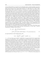
Heat Transfer at Reduced Flow Rate
The typical heating-only hydronic terminal gradually reduces its
heat output as flow is reduced (Figure 1). Decreasing water flow to
50% of design reduces the heat transfer to 90% of that at full design
flow. The control valve must reduce the water flow to 10% to reduce
the heat output to 50%. The reason for the relative insensitivity to
changing flow rates is that the governing coefficient for heat trans-
fer is the air-side coefficient. A change in internal or water-side
coefficient with flow rate does not materially affect the overall heat
transfer coefficient. This means that (1) heat transfer for water-to-
air terminals is established by the mean air-to-water temperature
difference, (2) the heat transfer is measurably changed, and (3) a
change in the mean water temperature requires a greater change in

the water flow rate.
A secondary concern also applies to heating terminals. Unlike
chilled water, hot water can be supplied at a wide range of temper-
atures. So, in some cases, an inadequate terminal heating capacity
caused by insufficient flow can be overcome by raising the supply
water temperature. Design below the temperature limit of 120°C
(ASME low-pressure boiler code) must be considered.
The previous comments apply to heating terminals selected
for a 10 K temperature drop (∆t) and with a supply water temper-
ature of about 93°C. Figure 2 shows the flow variation when 90%
terminal capacity is acceptable. Note that heating tolerance
decreases with temperature and flow rates and that chilled water
terminals are much less tolerant of flow variation than hot water
terminals.
Dual-temperature heating/cooling hydronic systems are some-
times completed and started during the heating season. Adequate
heating ability in the terminals may suggest that the system is bal-
anced. Figure 2 shows that 40% of design flow through the termi-
nal provides 90% of design heating with 60°C supply water and a
5 K temperature drop. Increased supply water temperature estab-
lishes the same heat transfer at terminal flow rates of less than 40%
design.
In some cases, dual-temperature water systems may experi-
ence a decreased flow during the cooling season because of the
chiller pressure drop; this could cause a flow reduction of 25%.
For example, during the cooling season, a terminal that originally
heated satisfactorily would only receive 30% of the design flow
rate.
While the example of reduced flow rate at ∆t = 10 K only affects
the heat transfer by 10%, this reduced heat transfer rate may have

the following negative effects:
1. The object of the system is to deliver (or remove) heat where
required. When the flow is reduced from the design rate, the sys-
tem must supply heating or cooling for a longer period to main-
tain room temperature.
2. As the load reaches design conditions, the reduced flow rate is
unable to maintain room design conditions.
Terminals with lower water temperature drops have a greater tol-
erance for unbalanced conditions. However, larger water flows are
necessary, requiring larger pipes, pumps, and pumping cost. Also,
automatic valve control is more difficult.
System balance becomes more important in terminals with a
large temperature difference. Less water flow is required, which
reduces the size of pipes, valves, and pumps, as well as pumping
costs. A more linear emission curve gives better system control.
Heat Transfer at Excessive Flow
The flow rate should not be increased above design in an effort to
increase heat transfer. Figure 3 shows that increasing the flow to
200% of design only increases heat transfer by 6% while increasing
the resistance or pressure drop 4 times and the power by the cube of
the original power (pump laws).
Generalized Chilled Water Terminal—
Heat Transfer Versus Flow
The heat transfer for a typical chilled water coil in an air duct ver-
sus water flow rate is shown in Figure 4. The curves shown are
based on ARI rating points: 7.2°C inlet water at a 5.6 K rise with
entering air at 26.7°C dry bulb and 19.4°C wet bulb.
The basic curve applies to catalog ratings for lower dry-bulb
temperatures providing a consistent entering air moisture content
(e.g., 23.9°C dry bulb, 18.3°C wet bulb). Changes in inlet water

temperature, temperature rise, air velocity, and dry- and wet-bulb
temperatures will cause terminal performance to deviate from the
curves. Figure 4 is only a general representation of the total heat
transfer change versus flow for a hydronic cooling coil and does
not apply to all chilled water terminals. Comparing Figure 4 with
Figure 1 indicates the similarity of the nonlinear heat transfer and
flow for both the heating and the cooling terminal.
Table 1 shows that if the coil is selected for the load, and the flow
is reduced to 90% of the load, three flow variations can satisfy the
reduced load at various sensible and latent combinations.
Fig. 1 Effects of Flow Variation on Heat Transfer
from a Hydronic Terminal
(Design ∆t = 10 K and supply temperature = 93°C)
Fig. 2 Percent of Design Flow Versus Design for
Various Supply Water Temperatures
36.10 1999 ASHRAE Applications Handbook (SI)
the desired curve can be determined from the manufacturer’s rat-
ings since these are published as (t
ew
− t
ea
). A second point is
established by observing that the heat transfer from air to water is
zero when (t
ew
− t
ea
) is zero (consequently, ∆t
w
= 0). With these

two points, an approximate performance curve can be drawn (see
Figure 6). Then, for any other (t
ew
− t
ea
), this curve is used to deter-
mine the appropriate ∆t
w
.
Example 1. From the following manufacturer certified data, determine the
required ∆t
w
:
Capacity = 3 kW
t
ew
= 95°C
t
ea
= 15°C
Water flow = 0.1 L/s
c
p
= 4.18 kJ/(kg·K)
ρ = 1.0 kg/L
Solution:
1. Calculate rated ∆t
w
.
2. Construct a performance curve as illustrated in Figure 6.

3. From test data:
4. From Figure 6 read ∆t
w
= 5.4 K, which is required to balance water flow
at 0.1 L/s. The water temperature difference may also be calculated as pro-
portion of the rate value as follows:
This procedure is useful for balancing terminal devices such as
finned tube convectors, where flow measuring devices do not exist
and where airflow measurements cannot be made. It may also be
used for cooling coils for sensible transfer (dry coil).
Flow Balancing by Total Heat Transfer. This procedure deter-
mines water flow by running an energy balance around the coil.
From field measurements of airflow, wet- and dry-bulb tempera-
tures both upstream and downstream of the coil, and the difference
∆t
w
between the entering and leaving water temperatures, water
flow can be determined by the following equations:
(5)
(6)
(7)
where
Q
w
= water flow rate, L/s
q = load, W
q
cooling
= cooling load, W
q

heating
= heating load, W
Q
a
= airflow rate, L/s
h = enthalpy, kJ/kg
t = temperature, °C
Example 2. Find the water flow for a cooling system having the following
characteristics:
Solution: From Equations (5) and (6),
The desired water flow is achieved by successive manual adjust-
ments and recalculations. Note that these temperatures can be
greatly influenced by the heat of compression, stratification,
bypassing, and duct leakage.
General Balance Procedures
All the variations of balancing hydronic systems cannot be
listed; however, the general method should balance the system
while minimizing operating cost. Excess pump pressure (excess
operating power) can be eliminated by trimming the pump impeller.
Allowing excess pressure to be absorbed by throttle valves adds a
lifelong operating cost penalty to the operation.
The following is a general procedure based on setting the balance
valves on the site:
1. Develop a flow diagram if one is not included in the design
drawings. Illustrate all balance instrumentation, and include
any additional instrument requirements.
2. Compare pumps, primary heat exchangers, and specified ter-
minal units; and determine whether a design diversity factor
can be achieved.
3. Examine the control diagram and determine the control adjust-

ments needed to obtain design flow conditions.
∆
t
w
3
4.18 0.1
×
1
×

7.18 K==
Fig. 6 Coil Performance Curve
t
ew
80
°
C=
t
ea
20
°
C=
t
ew
t
ea
–60
°
C=
t

ew
t
ea
–
()
test
t
ew
t
ea
–
()
rated

∆
t
w
()
rated
∆
t
w
()
required
=
80 20–
95 15–

7.18
×

5.4 K=
Test data
t
ewb
= entering wet-bulb temperature = 20.3°C
t
lwb
= leaving wet-bulb temperature = 11.9°C
Q
a
= airflow rate = 10 000 L/s
t
lw
= leaving water temperature = 15.0°C
t
ew
= entering water temperature = 8.6°C
From psychrometric chart
h
1
= 76.52 kJ/kg
h
2
= 52.01 kJ/kg
Q
w
Q 4180⁄∆t
w
=
q

cooling
1.20 Q
a
h
1
h
2
–()=
q
heating
1.23 Q
a
t
1
t
2
–()=
Q
w
1.20 10000 76.52 52.01–
()×
4180 15.0 8.6–
()

11.0 L/s==
36.12 1999 ASHRAE Applications Handbook (SI)
For example, a manufacturer may test a boiler control valve with
40°C water. Differential pressures from another test made in the
field at 120°C may be correlated with the manufacturer’s data by
using Equation (8) to account for the density differences of the two

tests.
When differential heads are used to estimate flow, a density cor-
rection must be made because of the shape of the pump curve. For
example, in Figure 8 the uncorrected differential reading for pumped
water with a density of 900 kg/m
3
is 25 m; the gage conversion was
assumed to be for water with a density of 999 kg/m
3
. The uncor-
rected or false reading gives a 40% error in flow estimation.
Differential Head Readout with Manometers
Manometers are used for differential pressure readout, especially
when very low differentials, great precision, or both, are required.
But manometers must be handled with care; they should not be used
for field testing because fluid could blow out into the water and rap-
idly deteriorate the components. A proposed manometer arrange-
ment is shown in Figure 9.
Figure 9 and the following instructions provide accurate manom-
eter readings with minimum risk of blowout.
1. Make sure that both legs of the manometer are filled with water.
2. Open the purge bypass valve.
3. Open valved connections to high and low pressure.
4. Open the bypass vent valve slowly and purge air here.
5. Open manometer block vents and purge air at each point.
6. Close the needle valves. The columns should zero in if the
manometer is free of air. If not, vent again.
7. Open the needle valves and begin throttling the purge bypass
valve slowly, watching the fluid columns. If the manometer has an
adequate available fluid column, the valve can be closed and the

differential reading taken. However, if the fluid column reaches
the top of the manometer before the valve is completely closed,
insufficient manometer height is indicated and further throttling
will blow fluid into the blowout collector. A longer manometer or
the single gage readout method should then be used.
An error is often introduced when converting millimetres of
gage fluid to the pressure difference (in kilopascals) of the test
fluid. The conversion factor changes with test fluid temperature,
density, or both. Conversion factors shown in Table 2 are to a water
base, and the counterbalancing water height H (Figure 9) is at room
temperature.
Orifice Plates, Venturi, and Flow Indicators
Manufacturers provide flow information for several devices used
in hydronic system balance. In general, the devices can be classified
as (1) orifice flowmeters, (2) venturi flowmeters, (3) velocity
impact meters, (4) pitot-tube flowmeters, (5) bypass spring impact
flowmeters, (6) calibrated balance valves, (7) turbine flowmeters,
and (8) ultrasonic flowmeters.
The orifice flowmeter is widely used and is extremely accurate.
The meter is calibrated and shows differential pressure versus flow.
Accuracy generally increases as the pressure differential across the
meter increases. The differential pressure readout instrument may
be a manometer, differential gage, or single gage (Figure 7).
The venturi flowmeter has lower pressure loss than the orifice
plate meter because a carefully formed flow path increases velocity
head recovery. The venturi flowmeter is placed in a main flow line
where it can be read continuously.
Velocity impact meters have precise construction and calibra-
tion. The meters are generally made of specially contoured glass or
plastic, which permits observation of a flow float. As flow

increases, the flow float rises in the calibrated tube to indicate flow
rate. Velocity impact meters generally have high accuracy.
A special version of the velocity impact meter is applied to
hydronic systems. This version operates on the velocity pressure
difference between the pipe side wall and the pipe center, which
causes fluid to flow through a small flowmeter. Accuracy depends
on the location of the impact tube and on a velocity profile that cor-
responds to theory and the laboratory test calibration base. Gener-
ally, the accuracy of this bypass flow impact or differential velocity
pressure flowmeter is less than a flow-through meter, which can
operate without creating a pressure loss in the hydronic system.
The pitot-tube flowmeter is also used for pipe flow measure-
ment. Manometers are generally used to measure velocity pressure
differences because these differences are low.
The bypass spring impact flowmeter uses a defined piping
pressure drop to cause a correlated bypass side branch flow. The
side branch flow pushes against a spring that increases in length
with increased side branch flow. Each individual flowmeter is cali-
brated to relate extended spring length position to main flow. The
bypass spring impact flowmeter has, as its principal merit, a direct
readout. However, dirt on the spring reduces accuracy. The bypass
Table 2 Differential Pressure Conversion to Head
Fluid Density,
kg/m
3
Approximate
Corresponding Water
Temperature, °C
Metre Fluid Head
Equal to 1 kPa

a
1500 0.680
1400 0.0728
1300 0.0784
1200 0.0850
1100 0.0927
1000 10 0.1020
980 65 0.104
960 95 0.106
940 125 0.108
920 150 0.111
900 170 0.113
800 0.127
700 0.146
600 0.170
500 0.204
a
Differential kPa readout is multiplied by this number to obtain metres fluid head
when gage is calibrated in kPa.
Fig. 9 Fluid Manometer Arrangement for
Accurate Reading and Blowout Protection
Testing, Adjusting, and Balancing 36.13
is opened only when a reading is made. Flow readings can be taken
at any time.
The calibrated balance valve is an adjustable orifice flowmeter.
Balance valves can be calibrated so that a flow/pressure drop rela-
tionship can be obtained for each incremental setting of the valve. A
ball, rotating plug, or butterfly valve may have its setting expressed
in percent open or degree open; a globe valve, in percent open or
number of turns. The calibrated balance valve must be manufac-

tured with precision and care to ensure that each valve of a particular
size has the same calibration characteristics.
The turbine flowmeter is a mechanical device. The velocity of
the liquid spins a wheel in the meter, which generates a 4 to 20 mA
output that may be calibrated in units of flow. The meter must be
well maintained, as wear or water impurities on the bearing may
slow the wheel, and debris may clog or break the wheel.
The ultrasonic flowmeter senses sound signals, which are cali-
brated in units of flow. The ultrasonic metering station may be
installed as part of the piping, or it may be a strap-on meter. In either
case, the meter has no moving parts to maintain, nor does it intrude
into the pipe and cause a pressure drop. Two distinct types of ultra-
sonic meter are available: (1) the transit time meter for HVAC or
clear water systems and (2) the Doppler meter for systems handling
sewage or large amounts of particulate matter.
If any of the above meters are to be useful, the minimum distance
of straight pipe upstream and downstream, as recommended by the
meter manufacturer and flow measurement handbooks, must be
adhered to. Figure 10 presents minimum installation suggestions.
Using a Pump as an Indicator
Although the pump is not a meter, it can be used as an indicator
of flow together with the other system components. Differential
pressure readings across a pump can be correlated with the pump
curve to establish the pump flow rate. Accuracy depends on (1)
accuracy of readout, (2) pump curve shape, (3) actual conformance
of the pump to its published curve, (4) pump operation without cav-
itation, (5) air-free operation, and (6) velocity pressure correction.
When a differential pressure reading must be taken, a single gage
with manifold provides the greatest accuracy (Figure 11). The pump
suction to discharge differential can be used to establish pump dif-

ferential pressure and, consequently, pump flow rate. The single
gage and manifold may also be used to check for strainer clogging
by measuring the pressure differential across the strainer.
If the pump curve is based on fluid head, pressure differential, as
obtained from the gage reading, needs to be converted to head,
which is pressure divided by the fluid density and gravity. The pump
differential head is then used to determine pump flow rate (Figure
12). As long as the differential head used to enter the pump curve is
expressed as head of the fluid being pumped, the pump curve shown
by the manufacturer should be used as described. The pump curve
may state that it was defined by test with 30°C water. This is unim-
portant, since the same curve applies from 15 to 120°C water, or to
any fluid within a broad viscosity range.
Generally, pump-derived flow information, as established by the
performance curve, is questionable unless the following precautions
are observed:
1. The installed pump should be factory calibrated by a test to
establish the actual flow-pressure relationship for that particular
pump. Production pumps can vary from the cataloged curve
because of minor changes in impeller diameter, interior casting
tolerances, and machine fits.
2. When a calibration curve is not available for a centrifugal pump
being tested, the discharge valve can be closed briefly to estab-
lish the no-flow shutoff pressure, which can be compared to the
published curve. If the shutoff pressure differs from that pub-
lished, draw a new curve parallel to the published curve. While
not exact, the new curve will usually fit the actual pumping
circumstance more accurately. Clearance between the impeller
and casing minimize the danger of damage to the pump during a
no-flow test, but manufacturer verification is necessary.

3. Differential pressure should be determined as accurately as pos-
sible, especially for pumps with flat flow curves.
4. The pump should be operating air-free and without cavitation.
A cavitating pump will not operate to its curve, and differential
readings will provide false results.
5. Ensure that the pump is operating above the minimum net posi-
tive suction pressure.
6. Power readings can be used (1) as a check for the operating
point when the pump curve is flat or (2) as a reference check
when there is suspicion that the pump is cavitating or providing
false readings because of air.
Fig. 10 Minimum Installation Dimensions for Flowmeter
Fig. 11 Single Gage for Differential Readout Across
Pump and Strainer
Fig. 12 Differential Pressure Used to Determine Pump Flow
Testing, Adjusting, and Balancing 36.17
Data sheets needed for energy conservation field surveys con-
tain different and, in some cases, more comprehensive information
than those used for testing, adjusting, and balancing. Generally,
the energy engineer determines the degree of fieldwork to be per-
formed; data sheets should be compatible with the instructions
received.
Building Systems
The most effective way to reduce building energy waste is to
identify, define, and tabulate the energy load by building system.
For this purpose, load is defined as the quantity of energy used in a
building, or by one of its subsystems, for a given period. By follow-
ing this procedure, the most effective energy conservation opportu-
nities can be achieved more quickly because high priorities can be
assigned to systems that consume the most energy.

A building can be divided into nonenergized systems and ener-
gized systems. Nonenergized systems do not require outside energy
sources such as electricity and fuel. Energized systems (e.g.,
mechanical and electrical systems) require outside energy. Ener-
gized and nonenergized systems can be divided into subsystems
defined by function. Nonenergized subsystems are (1) building site,
envelope, and interior; (2) building use; and (3) building operation.
Building Site, Envelope, and Interior. The site, envelope, and
interior should be surveyed to determine how they can be modified
to reduce the building load that the mechanical and electrical sys-
tems must meet without adversely affecting the building’s appear-
ance. It is important to compare actual conditions with conditions
assumed by the designer, so that the mechanical and electrical sys-
tems can be adjusted to balance their capacities to satisfy actual
needs.
Building Use. These loads can be classified as people occupancy
loads or people operation loads. People occupancy loads are related
to schedule, density, and mixing of occupancy types (e.g., process
and office). People operation loads are varied, and include (1) oper-
ation of manual window shading devices; (2) setting of room ther-
mostats; and (3) conservation-related habits such as turning off
lights, closing doors and windows, turning off energized equipment
when not in use, and not wasting domestic hot or chilled water.
Building Operation. This subsystem consists of the operation
and maintenance of all the building subsystems. The load on the
building operation subsystem is affected by factors such as (1) the
time at which janitorial services are performed, (2) janitorial crew
size and time required to clean, (3) amount of lighting used to
perform janitorial functions, (4) quality of the equipment mainte-
nance program, (5) system operational practices, and (6) equip-

ment efficiencies.
Building Energized Systems
The energized subsystems of the building are generally plumb-
ing, heating, ventilating, cooling, space conditioning, control, elec-
trical, and food service. Although these systems are interrelated and
often use common components, logical organization of data
requires evaluating the energy use of each subsystem as indepen-
dently as possible. In this way, proper energy conservation mea-
sures for each subsystem can be developed.
Process Loads
In addition to building subsystem loads, the process load in most
buildings must be evaluated by the energy field auditor. Most tasks
not only require energy for performance, but also affect the energy
consumption of other building subsystems. For example, if a pro-
cess releases large amounts of heat to the space, the process con-
sumes energy and also imposes a large load on the cooling system.
Guidelines for Developing a Field Study Form
A brief checklist follows that outlines requirements for a field
study form needed to conduct an energy audit.
Inspection and Observation of All Systems. Record physical
and mechanical condition of the following:
• Fan blades, fan scroll, drives, belt tightness, and alignment
• Filters, coils, and housing tightness
• Ductwork (equipment room and space, where possible)
•Strainers
• Insulation ducts and piping
• Makeup water treatment and cooling tower
Interview of Physical Plant Supervisor. Record answers to the
following survey questions:
• Is the system operating as designed? If not, what changes have

been made to ensure its performance?
• Have there been modifications or additions to the system?
• If the system has been a problem, list problems by frequency of
occurrence.
• Are any systems cycled? If so, which systems and when, and
would building load permit cycling systems?
Recording System Information. Record the following system/
equipment identification:
• Type of system—single-zone, multizone, double-duct, low- or
high-velocity, reheat, variable volume, or other
• System arrangement—fixed minimum outside air, no relief, grav-
ity or power relief, economizer gravity relief, exhaust return, or
other
• Air-handling equipment—fans (supply, return, and exhaust):
manufacturer, model, size, type, and class; dampers (vortex,
scroll, or discharge); motors: manufacturer, power requirement,
full load amperes, voltage, phase, and service factor
• Chilled and hot water coils—area, tubes on face, fin spacing, and
number of rows (coil data necessary when shop drawings are not
available)
• Terminals—high-pressure mixing box: manufacturer, model, and
type (reheat, constant volume, variable volume, induction);
grilles, registers, and diffusers: manufacturer, model, style, and
loss coefficient to convert field-measured velocity to flow rate
• Main heating and cooling pumps, over 3.5 kW—manufacturer,
pump service and identification, model, size, impeller diameter,
speed, flow rate, head at full flow, and head at no flow; motor
data: power, speed, voltage, amperes, and service factor
• Refrigeration equipment—chiller manufacturer, type, model,
serial number, nominal tons, input power, total heat rejection,

motor (kilowatts, amperes, volts), chiller pressure drop, entering
and leaving chilled water temperatures, condenser pressure drop,
condenser entering and leaving water temperatures, running
amperes and volts, no-load running amperes and volts
• Cooling tower—manufacturer, size, type, nominal cooling capac-
ity, range, flow rate, and entering wet-bulb temperature
• Heating equipment—boiler (small through medium) manufac-
turer, fuel, energy input (rated), and heat output (rated)
Recording Test Data. Record the following test data:
• Systems in normal mode of operation (if possible)—fan motor:
running amperes and volts and power factor (over 3.5 kW); fan:
speed, total air (pitot-tube traverse where possible), and static
pressure (discharge static minus inlet total); static profile drawing
(static pressure across filters, heating coil, cooling coil, and
dampers); static pressure at ends of runs of the system (identify-
ing locations)
• Cooling coils—entering and leaving dry- and wet-bulb tempera-
tures, entering and leaving water temperatures, coil pressure drop
(where pressure taps permit and manufacturer’s ratings can be
Testing, Adjusting, and Balancing 36.19
Background sound measurements generally have to be made (1)
when the specification requires that the sound levels from HVAC
equipment only, as opposed to the sound level in a space, not exceed
a certain specified level; (2) when the sound level in the space
exceeds a desirable level, in which case the noise contributed by the
HVAC system must be determined; and (3) in residential locations
where little significant background noise is generated during the
evening hours and where generally low allowable noise levels are
specified or desired. Because background noise from outside
sources such as vehicular traffic can fluctuate widely, sound mea-

surements for residential locations are best made in the normally
quiet evening hours.
Sound Testing
Ideally, a building should be completed and ready for occupancy
before sound level tests are taken. All spaces in which readings will
be taken should be furnished with drapes, carpeting, and furniture,
as these affect the room absorption and the subjective quality of the
sound. In actual practice, since most tests have to be conducted
before the space is completely finished and furnished for final occu-
pancy, the testing engineer must make some allowances. Because
furnishings increase the absorption coefficient and reduce to 4 dB
the sound pressure level that can be expected between most live and
dead spaces, the following guidelines should suffice for measure-
ments made in unfurnished spaces. If the sound pressure level is
5 dB or more over specified or desired criterion, it can be assumed
that the criterion will not be met, even with the increased absorption
provided by furnishings. If the sound pressure level is 0 to 4 dB
greater than specified or desired criterion, recheck when the room is
furnished to determine compliance.
Follow this general procedure:
1. Obtain a complete set of accurate, as-built drawings and specifi-
cations, including duct and piping details. Review specifications
to determine sound and vibration criteria and any special instruc-
tions for testing.
2. Visually check for noncompliance with plans and specifications,
obvious errors, and poor workmanship. Turn system on for aural
check. Listen for noise and vibration, especially duct leaks and
loose fittings.
3. Adjust and balance equipment, as described in other sections, so
that final acoustical tests are made with the HVAC as it will be

operating. It is desirable to perform acoustical tests for both sum-
mer and winter operation, but where this is not practical, make
tests for the summer operating mode, as it usually has the poten-
tial for higher sound levels. Tests must be made for all mechan-
ical equipment and systems, including standby.
4. Check calibration of instruments.
5. Measure sound levels in all areas as required, combining mea-
surements as indicated in item 3 if equipment or systems must be
operated separately. Before final measurements are made in any
particular area, survey the area using an A-weighted scale read-
ing (dBA) to determine the location of the highest sound pres-
sure level. Indicate this location on a testing form, and use it for
test measurements. Restrict the preliminary survey to determine
location of test measurements to areas that can be occupied by
standing or sitting personnel. For example, measurements would
not be made directly in front of a diffuser located in the ceiling,
but they would be made as close to the diffuser as standing or sit-
ting personnel might be situated. In the absence of specified
sound criteria, the testing engineer should measure sound pres-
sure levels in all occupied spaces to determine compliance with
criteria indicated in Chapter 46 and to locate any sources of
excessive or disturbing noise.
6. Determine whether background noise measurements must be
made.
(a) If specification requires determination of sound level from
HVAC equipment only, it will be necessary to take back-
ground noise readings by turning HVAC equipment off.
(b) If specification requires compliance with a specific noise
level or criterion (e.g., sound levels in office areas shall not
exceed 35 dBA), ambient noise measurements must be made

only if the noise level in any area exceeds the specified
value.
(c) For residential locations and areas requiring very low noise,
such as sound recording studios and locations that are used
during the normally quieter evening hours, it is usually
desirable to take sound measurements in the evening and/or
take ambient noise measurements.
7. For outdoor noise measurements to determine noise radiated by
outdoor or roof-mounted equipment such as cooling towers and
condensing units, the section on Sound Control for Outdoor
Equipment in Chapter 46, which presents proper procedure and
necessary calculations, should be consulted.
Noise Transmission Problems
Regardless of the precautions taken by the specifying engineer
and the installing contractors, situations can occur where the sound
level exceeds specified or desired levels, and there will be occa-
sional complaints of noise in completed installations. A thorough
understanding of Chapter 46 and the section on Testing for Vibra-
tion in this chapter is desirable before attempting to resolve any
noise and vibration transmission problems. The following is
intended as an overall guide rather than a detailed problem-solving
procedure.
All noise transmission problems can be evaluated in terms of the
source-path-receiver concept. Objectionable transmission can be
resolved by (1) reducing the noise at the source by replacing defec-
tive equipment, repairing improper operation, proper balancing and
adjusting, and replacing with quieter equipment; (2) attenuating the
paths of transmission with silencers, vibration isolators, and wall
treatment to increase transmission loss; and (3) reducing or masking
objectionable noise at the receiver by increasing room absorption or

introducing a nonobjectionable masking sound. The following dis-
cussion includes (1) ways to identify actual noise sources using sim-
ple instruments or no instruments and (2) possible corrections.
When troubleshooting in the field, the engineer should listen to
the offending sound. The best instruments are no substitute for care-
ful listening, as the human ear has the remarkable ability to identify
certain familiar sounds such as bearing squeak or duct leaks and is
able to discern small changes in frequency or sound character that
might not be apparent from meter readings only. The ear is also a
good direction and range finder; because noise generally gets louder
as one approaches the source, direction can often be determined by
turning the head. Hands can also identify noise sources. Air jets from
duct leaks can often be felt, and the sound of rattling or vibrating pan-
els or parts often changes or stops when these parts are touched.
In trying to locate noise sources and transmission paths, the
engineer should consider the location of the affected area. In areas
that are remote from equipment rooms containing significant noise
producers but adjacent to shafts, noise is usually the result of struc-
ture-borne transmission through pipe and duct supports and
anchors. In areas adjoining, above, or below equipment rooms,
noise is usually caused by openings (acoustical leaks) in the sepa-
rating floor or wall or by improper, ineffective, or maladjusted
vibration isolation systems.
Unless the noise source or path of transmission is quite obvious,
the best way to identify it is by eliminating all sources systemati-
cally as follows:
1. Turn off all equipment to make sure that the objectionable
noise is caused by the HVAC. If the noise stops, the HVAC
components (compressors, fans, and pumps) must be operated
Testing, Adjusting, and Balancing 36.21

Reed vibrometers are relatively inexpensive instruments often
used for testing vibration, but relative inaccuracy limits their use-
fulness.
Vibrometers are moderately priced instruments that measure
vibration amplitude by means of a light beam projected on a grad-
uated scale.
Vibration meters are moderately priced electronic instruments
that measure vibration amplitude on a meter scale and are simple to
use.
Vibrographs are moderately priced mechanical instruments that
measure both amplitude and frequency. They are useful for analysis
and testing because they provide a chart recording showing ampli-
tude, frequency, and actual wave form of vibration. They can be
used for simple yet accurate determination of the natural frequency
of shafts, components, and systems by a bump test.
Vibration analyzers are relatively expensive electronic instru-
ments that measure amplitude and frequency, usually incorporating
a variable filter.
Strobe lights are often used with many of the aforementioned
instruments for analyzing and balancing rotating equipment.
Stethoscopes that amplify sound are available as inexpensive
mechanic’s type (basically, a standard stethoscope with a probe
attachment); relatively inexpensive types incorporating a tuneable
filter; and moderately priced powered types that electronically
amplify sound and provide some type of meter and/or chart re-
cording. Stethoscopes are often used to determine whether bear-
ings are bad.
The choice of instruments depends on the test. A stethoscope
should be part of every tester’s kit as it is one of the most practical,
yet least expensive, instruments and one of the best means of check-

ing bearings. Vibrometers and vibration meters can be used to mea-
sure vibration amplitude as an acceptance check. Since they cannot
measure frequency, they cannot be used for analysis and primarily
function as a go-no-go instrument. The best acceptance criteria con-
sider both amplitude and frequency. However, because vibrometers
and vibration meters are moderately priced and easy to use, they are
widely used. Anyone seriously concerned with vibration testing
should use an instrument that can determine frequency as well as
amplitude, such as a vibrograph or vibration analyzer.
Testing Vibration Isolation
The following steps should be taken to ensure that vibration iso-
lators are functioning properly:
1. Ensure that the equipment is free floating by applying an unbal-
anced load, which should cause the equipment to move freely
and easily. On floor-mounted equipment, check that there are no
obstructions between the base or foundation and the building
structure that would cause transmission while still permitting
equipment to rock relatively free because of the application of an
unbalanced force (Figure 13). On suspended equipment, check
that hanger rods are not touching the hanger. Rigid connections
such as pipes and ducts can prohibit mounts from functioning
properly and from providing a transmission path. Note that the
fact that the equipment is free floating does not mean that the iso-
lators are functioning properly. For example, a 500 rpm fan
installed on isolators having a natural frequency of 500 cycles
per minute (8.33 Hz) could be free floating but would actually be
in resonance, resulting in transmission to the building and exces-
sive movement.
2. Determine whether isolators are adjusted properly and providing
desired isolation efficiency. All isolators supporting a piece of

equipment should have approximately the same deflection (i.e.,
they should be compressed the same under the equipment). If
not, they have been improperly adjusted, installed, or selected;
this should be corrected immediately. Note that isolation effi-
ciency cannot be checked by comparing vibration amplitude on
equipment to amplitude on the structure (Figure 14).
The only accurate check of isolation efficiencies is to compare
vibration measurements of equipment operating with isolators to
measurements of equipment operating without isolators. Because
this type of test is usually impractical, it is better to check
whether the isolator’s deflection is as specified and whether the
specified or desired isolation efficiency is being provided. Figure
15 shows natural frequency of isolators as a function of deflec-
tion and indicates the theoretical isolation efficiencies for various
frequencies at which the equipment operates.
While it is easy to determine the deflection of spring mounts by
measuring the difference between the free heights with a ruler
(information as shown on submittal drawings or available from a
manufacturer), such measurements are difficult with most pad or
rubber mounts. Further, most pad and rubber mounts do not lend
themselves to accurate determination of natural frequency as a func-
tion of deflection. For such mounts, the most practical approach is
to check that there is no excessive vibration of the base and no
noticeable or objectionable vibration transmission to the building
structure.
If isolators are in the 90% efficiency range, and there is transmis-
sion to the building structure, either the equipment is operating
roughly or there is a flanking path of transmission, such as connect-
ing piping or obstruction, under the base.
Testing Equipment Vibration

Testing equipment vibration is necessary as an acceptance check
to determine whether equipment is functioning properly and to
ensure that objectionable vibration and noise are not transmitted.
Although a person familiar with equipment can determine when it is
Fig. 13 Obstructed Isolation Systems
Fig. 14 Testing Isolation Efficiency
Testing, Adjusting, and Balancing 36.23
condition of resonance, i.e., some part having a natural fre-
quency close to the operating speed, resulting in greatly ampli-
fied levels of vibration.
A bent shaft or eccentricity usually causes imbalance that
results in significantly higher vibration amplitude at lower
speeds, as shown in Figure 17, whereas vibration caused by
imbalance generally increases as speed increases.
If a bent shaft or eccentricity is suspected, check the dial indi-
cator. A bent shaft or eccentricity between bearings as shown in
Figure 18A can usually be compensated for by field balancing,
although some axial vibration might remain. Field balancing
cannot correct vibration caused by a bent shaft on direct-con-
nected equipment, on belt-driven equipment where the shaft is
bent at the location of sheave, or if the sheave is eccentric (Figure
18B). This is because the center-to-center distance of the sheaves
will fluctuate, each revolution resulting in vibration.
2. For belt- or gear-driven equipment where vibration is at
motor driving frequency rather than driven speed, it is best to
disconnect the drive to perform tests. If the vibration ampli-
tude of the motor operating by itself does not exceed speci-
fied or allowable values, excessive vibration (when the drive
is connected) is probably a function of bent shaft, misalign-
ment, eccentricity, resonance, or loose hold-down bolts.

3. Vibration caused by imbalance can be corrected in the field by
firms specializing in this service or by testing personnel if they
have appropriate equipment and experience.
Vibration at Other than Rotational Frequency. Vibration at
frequencies other than driving and driven speeds is generally
considered unacceptable. Table 4 shows some common conditions
that can cause vibration at other than rotational frequency.
Resonance. If resonance is suspected, determine which part of
the system is in resonance.
Isolation Mounts. The natural frequency of the most commonly
used spring mounts is a function of spring deflection, as shown in
Figure 11 in Chapter 7 of the 1997 ASHRAE Handbook—Funda-
mentals, and it is relatively easy to calculate by determining the dif-
ference between the free and operating height of the mount, as
explained in the section on Testing Vibration Isolation. This tech-
nique cannot be applied to rubber, pad, or fiberglass mounts, which
have a natural frequency in the 5 to 50 Hz range. Natural frequency
for such mounts is determined by a bump test. Any resonance with
isolators should be immediately corrected as it results in excessive
movement of equipment and more transmission to the building
structure than if equipment were attached solidly to the building
(installed without isolators).
Components. Resonance can occur with any shaft, structural
base, casing, and connected piping. The easiest way to determine
natural frequency is to perform a bump test with a vibrograph. This
test consists of bumping the part and measuring with an instrument;
the part will vibrate at its natural frequency, which is recorded on
instrument chart paper. Similar tests, though not as convenient or
accurate, can be made with a reed vibrometer or a vibration ana-
lyzer. However, most of these instruments are restricted to frequen-

cies above 8.3 Hz. They therefore cannot be used to determine
natural frequencies of most isolation systems, which usually have
natural frequencies lower than 8.3 Hz.
Checking for Vibration Transmission. The source of vibration
transmission can be checked by determining frequency with a vibra-
tion analyzer and tracing back to equipment operating at this speed.
However, the easiest and usually the best method (even if test equip-
ment is being used) is to shut off components one at a time until the
source of transmission is located. Most transmission problems
cause disturbing noise; listening is the most practical approach to
determine a noise source because the ear is usually better than
sound-measuring instruments at distinguishing small differences
and changes in character and amount of noise. Where disturbing
transmission consists solely of vibration, a measuring instrument
will probably be helpful, unless vibration is significantly above the
Table 4 Common Causes of Vibration Other than
Unbalance at Rotation Frequency
Frequency Source
0.5 × rpm Vibration at approximately 0.5 rpm can result from improp-
erly loaded sleeve bearings. This vibration will usually dis-
appear suddenly as equipment coasts down from operating
speed.
2 × rpm Equipment is not tightly secured or bolted down.
2 × rpm Misalignment of couplings or shafts usually results in vibra-
tion at twice rotational frequency and generally a relatively
high axial vibration.
Many × rpm Defective antifriction (ball, roller) bearings usually result in
low-amplitude, high-frequency, erratic vibration. Because
defective bearings usually produce noise rather than any
significantly measurable vibration, it is best to check all

bearings with a stethoscope or similar listening device.
Fig. 16 Vibration from Resonant Condition
Fig. 17 Vibration Caused by Eccentricity
Fig. 18 Bent Shafts
36.24 1999 ASHRAE Applications Handbook (SI)
sensory level of perception. Vibration below the sensory level of
perception is generally not objectionable.
If equipment is located near the affected area, check isolation
mounts and equipment vibration. If vibration is not being transmit-
ted through the base, or if the affected area is remote from equip-
ment, the probable cause is transmission through connected piping
and/or ducts. Ducts can usually be isolated by isolation hangers.
However, transmission through connected piping is very common
and presents numerous problems that should be understood before
attempting to correct them as discussed in the following section.
Vibration and Noise Transmission in Piping
Vibration and noise in connected piping can be generated by
either equipment (e.g., pump or compressor) or flow (velocity).
Mechanical vibration due to equipment can be transmitted through
the walls of pipes or by a water column. Flexible pipe connectors,
which provide system flexibility to permit isolators to function
properly and protect equipment from stress caused by misalignment
and thermal expansion, can be useful in attentuating mechanical
vibration transmitted through a pipe wall. However, they rarely sup-
press flow vibration and noise and only slightly attenuate mechan-
ical vibration as transmitted through a water column.
Tie rods are often used with flexible rubber hose and rubber
expansion joints (Figure 19). While they accommodate thermal
movements, they hinder the isolation of vibration and noise. This is
because pressure in the system causes the hose or joint to expand

until resilient washers under tie rods are virtually rigid. To isolate
noise adequately with a flexible rubber connector, tie rods and
anchor piping should not be used. However, this technique gener-
ally cannot be used with pumps that are on spring mounts because
they would still permit the hose to elongate. Flexible metal hose can
be used with spring-isolated pumps since wire braid serves as tie
rods; metal hose controls vibration but not noise.
Problems of transmission through connected piping are best
resolved by changes in the system to reduce noise (improve flow
characteristics, turn down impeller) or by completely isolating pip-
ing from the building structure. Note, however, that it is almost
impossible to isolate piping completely from the structure, as
required resiliency is inconsistent with rigidity requirements of pipe
anchors and guides. Chapter 46 contains information on flexible
pipe connectors and resilient pipe supports, anchors, and guides,
which should help resolve any piping noise transmission problems.
REFERENCES
AMCA. 1985. Laboratory methods of testing fans for rating. Standard 210-
85. Also ASHRAE Standard 51-1985. Air Movement and Control Asso-
ciation, Arlington Heights, IL.
ASHRAE. 1988. Practices for measurement, testing, adjusting and balanc-
ing of building heating, ventilation, air conditioning and refrigeration
systems. Standard 111-1988.
ASHRAE. 1991. Terminology of heating, ventilation, air conditioning, and
refrigeration, 2nd ed.
ASME. 1986. Atmospheric water cooling equipment. Standard PTC 23-86.
American Society of Mechanical Engineers, New York.
ASME. 1988. Boiler and pressure vessel code, Section VI. American Soci-
ety of Mechanical Engineers, New York, NY.
CTI. 1997. Standard specifications for thermal testing of wet/dry cooling

towers. Standard Specification ATC-105. Cooling Tower Institute,
Houston, TX.
Griggs, E.I., W.B. Swim, and H.G. Yoon. 1990. Placement of air control sen-
sors. ASHRAE Transactions 96(1).
Sauer, H.J. and R.H. Howell. 1990. Airflow measurements at coil faces with
vane anemometers: Statistical correction and recommended field mea-
surement procedure. ASHRAE Transactions 96(1):502-11.
BIBLIOGRAPHY
AABC. 1989. National standards for total system balance, 5th ed. Associ-
ated Air Balance Council, Washington, D.C.
AABC. 1997. Testing and balancing procedures. Associated Air Balance
Council, Washington, D.C.
AMCA. 1987. Fan application manual. Air Movement and Control Asso-
ciation, Arlington Heights, IL.
Armstrong Pump. 1986. Technology of balancing hydronic heating and
cooling systems. Armstrong Pump, North Tonawanda, NY.
ASA. 1983. Specification for sound level meters. Standard 1.4-83. Acous-
tical Society of America, New York.
ASHRAE. 1996. The HVAC commissioning process. Guideline 1-1996.
Coad, W.J. 1985. Variable flow in hydronic systems for improved stability,
simplicity and energy economics. ASHRAE Transactions 91(1B):224-
37.
Eads, W.G. 1983. Testing, balancing and adjusting of environmental sys-
tems. In Fan Engineering, 8th ed. Buffalo Forge Company, Buffalo, NY.
Gladstone, J. 1981. Air conditioning—Testing and balancing: A field prac-
tice manual. Van Nostrand Reinhold, New York.
Gupton, G. 1989. HVAC controls, operation and maintenance. Van Nostrand
Reinhold, New York.
Haines, R.W. 1987. Control systems for heating, ventilating and air condi-
tioning, 4th ed. Van Nostrand Reinhold, New York.

Hansen, E.G. 1985. Hydronic system design and operation. McGraw-Hill,
New York.
Miller, R.W. 1983. Flow measurement engineering handbook. McGraw-
Hill, New York.
NEBB. 1991. Procedural standards for testing, balancing and adjusting of
environmental systems, 5th ed. National Environmental Balancing
Bureau, Vienna, VA.
NEBB. 1986. Testing, adjusting, balancing manual for technicians, 1st ed.
SMACNA. 1993. HVAC systems—Testing, adjusting and balancing, 2nd ed.
Sheet Metal and Air Conditioning Contractors’ National Association,
Merrifield, VA.
SMACNA. 1995. HVAC air duct leakage test manual
, 1st ed.
Trane Company. 1988. Trane air conditioning manual. The Trane Company,
LaCrosse, WI.
Fig. 19 Typical Tie Rod Assembly
CHAPTER 37
OPERATION AND MAINTENANCE MANAGEMENT
Terminology 37.1
Quantitative Management Concept 37.1
Documentation 37.2
Maintenance Management 37.3
Knowledge and Skills 37.3
Levels of Effort 37.3
Condition Monitoring 37.4
Condition-Based Maintenance 37.4
Responsibilities 37.4
New Technology 37.5
LTHOUGH mechanical maintenance was once the responsi-
Ability of trained technical personnel, increasingly sophisti-

cated systems and equipment require overall management programs
to handle organization, staffing, planning, and control. These pro-
grams should meet present and future personnel and technical
requirements. They must also meet system availability and energy
use requirements. Additionally, they must upgrade management
and operator skills, and increase communication among those who
benefit from cost-effective operation and maintenance.
Good maintenance management planning includes proper cost
analysis and a process to ensure that occupant comfort, energy plan-
ning, and safety and security systems are optimal for all facilities.
Appropriate technical expertise, whether in-house or contracted, is
also important. This chapter addresses the following issues:
• Cost-effectiveness
• Commissioning
• Management approaches according to the criticality of buildings
or systems
• Documentation and record keeping
• Condition monitoring and maintenance
• Operation and maintenance responsibilities of designers, contrac-
tors, manufacturers/suppliers, and owners
Operation and maintenance of all HVAC&R systems should be
considered during the original design of a building. Any successful
operation and maintenance program must include proper documen-
tation of the design intent and criteria. ASHRAE Guideline 4 pro-
vides a methodology to properly document HVAC systems. Newly
installed systems must be commissioned to ensure that they are
functioning as designed. ASHRAE Guideline 1 provides the meth-
ods and procedures for HVAC system commissioning. It is then the
responsibility of the management and operational staff to retain the
design function throughout the life of the building. Existing systems

may need to be recommissioned to accommodate changes.
TERMINOLOGY
System operation defines the parameters under which the build-
ing or systems operator can adjust components of the system to sat-
isfy the tenant comfort or process requirements and the strategy for
optimum energy use and minimum maintenance.
The maintenance program defines maintenance in terms of
time and resource allocation. It documents the objectives, estab-
lishes evaluation criteria, and commits the maintenance department
to basic areas of performance, such as prompt response to mechan-
ical failure and attention to planned functions that protect capital
investment and minimize downtime or failure response.
Failure response classifies maintenance department resources
expended or reserved to handle interruptions in the operation or func-
tion of a system or equipment covered by the maintenance program.
This classification includes two response types—repair and service.
Repair is to make good, or to restore to good or sound condition
with the following constraints: (1) operation must be fully restored
without embellishment, and (2) failure must trigger the response.
Service provides what is necessary to effect a maintenance pro-
gram short of repair. It is usually based on manufacturers’ recom-
mended procedures.
Planned maintenance classifies maintenance department
resources that are invested in prudently selected functions at speci-
fied intervals. All functions and resources within this classification
must be planned, budgeted, and scheduled. Planned maintenance
embodies two concepts—preventive and corrective maintenance.
Preventive maintenance classifies resources allotted to ensure
proper operation of a system or equipment under the maintenance
program. Durability, reliability, efficiency, and safety are the prin-

cipal objectives.
Corrective maintenance classifies resources, expended or
reserved, for predicting and correcting conditions of impending fail-
ure. Corrective action is strictly remedial and always performed
before failure occurs. An identical procedure performed in response
to failure is classified as a repair. Corrective action may be taken
during a shutdown caused by failure, provided the action is optional
and unrelated.
Predictive maintenance is a function of corrective maintenance.
Statistically supported objective judgment is implied. Nondestruc-
tive testing, chemical analysis, vibration and noise monitoring, and
routine visual inspection and logging are classified under this func-
tion, provided that the item tested or inspected is part of the planned
maintenance program.
Durability is the average expected service life of a system or
facility. Table 3 in Chapter 35 lists median years of service life of
various equipment. Individual manufacturers quantify durability as
design life, which is the average number of hours of operation
before failure, extrapolated from accelerated life tests and from
stressing critical components to economic destruction.
Reliability is the probability that a system or facility will per-
form its intended function for a specified period of time when used
under specific conditions and environment.
QUANTITATIVE MANAGEMENT CONCEPT
The following life-cycle management concept is recommended
for operation and maintenance program planning. The concept can
be used during the construction cycle as well as for day-to-day
operation and maintenance management. Derived from value engi-
neering, this life-cycle concept of management (see Figure 1) in-
volves three interdependent dimensions: effectiveness (value),

durability (time), and life-cycle cost (money). Their numerical val-
ues are affected by the type and extent of the operation and mainte-
nance programs.
System effectiveness is the ability of a system to perform its
intended use in terms of performance, availability, and dependabil-
ity. To be perfectly effective, a facility must provide the required
services satisfactorily and must operate dependably without failure
The preparation of this chapter is assigned to TC 1.7, Operation and
Maintenance Management.
CHAPTER 38
COMPUTER APPLICATIONS
Application Concepts 38.1
General Productivity Tools 38.3
Engineering Design Calculations 38.4
Simulation Programs 38.8
Graphics Applications 38.9
Monitoring and Control 38.10
Applications of Artificial
Intelligence 38.11
Internet 38.12
ASHRAE Developed Software 38.13
HE use of computers in the heating, refrigerating, and air-
Tconditioning industry has come about because of the variety of
engineering analysis programs for the HVAC industry, an even
larger number and range of programs for business use, and the low
cost of powerful computers on which to run them. The ordinary cal-
culations required in the HVAC industry, such as heating and cool-
ing loads, can be performed easily and inexpensively on a computer.
In addition, computers sometimes allow the solution of more com-
plex problems that would otherwise be impractical to solve. The

operation and maintenance of buildings has also benefited from
computers that monitor, control, and in certain cases diagnose prob-
lems in HVAC equipment. This chapter covers computer concepts
for both general and specialized application to the HVAC industry.
APPLICATION CONCEPTS
Current technology in the computer industry changes rapidly. By
the time a computer is purchased and implemented, new technology
may appear on the market that renders it obsolete. This situation,
along with the need to share information and applications among
various computers, makes a design that can readily adapt to change
a necessity. An information system has an architecture in much the
same way that a building does. If laid out properly, this architecture
can accommodate the introduction of new technologies while
allowing the continuing use of existing software.
Before choosing computer products, the business that the infor-
mation system will serve must be understood. End users can best
specify the principles most important to a particular business. The
system and applications can then be selected to match the needs of
the business, and a technical framework that supports a consistent
computing environment can be established.
Standards take several forms. Industry standards, such as ISO,
ANSI/IEEE, and SQL, are defined and recognized by industry
groups. Proprietary standards are often formed where other stan-
dards are not applicable, such as in a company. De facto standards,
such as the operating system software for personal computers, are
another type of standard.
Hardware
The availability of inexpensive personal computers and worksta-
tions at prices affordable to any company has made in-house com-
puting an attractive option for even the smallest firm. The obvious

advantages of rapid turnaround and unlimited computing for a fixed
investment are compelling.
A personal computer operates at low cost to allow interactive
usage and storage for the tasks a user generally takes on. Data can
be transferred to other computers. This combination can enable a
firm to handle a larger number and variety of projects than would be
possible with a central system alone.
But owning a computer incurs additional expenses, including
maintenance, software, and personnel costs. Software must be
either bought or developed, and although it may seem expensive to
buy, it is almost always more expensive to develop. A firm should
employ at least one person knowledgeable about the systems and
the software, or have contractual access to such a person.
Personal and workstation computers offer the small office enor-
mous power at low cost. These machines should be considered in
the class of business machines, in that they offer more possibilities
than technical analysis (see the section on General Productivity
Tools).
Laptop computers are battery-powered, miniature personal
computers that are fully functional and more or less portable. These
computers are also called palmtops, portables, or notebooks
depending on their size.
Any of the hardware options described here may be connected
through a local-area network (LAN), or a wide-area network
(WAN). When machines are thus connected, one or more of the
computers may be used as a file server. Any computer, once con-
nected locally or via telephone to the server, has access to common
data and programs through the network. This method allows data
stored in one logical database to be accessed from many separate
computers without the necessity of copying the data onto numerous

storage devices.
An emerging hardware technology is parallel processing. In
this computing method, the processors in one or more networked
computers are used in parallel, each solving a portion of a problem.
A control program determines what processing power is needed and
available for a particular computational task. The task is then
assigned to a processor. When the computation is complete, the
results are passed back. Depending on the system and the control
program, several software program steps may be completed at the
same time. This method shows great promise in the area of simula-
tions, which tend to be computationally intensive and which may be
easily divided into smaller pieces.
Personal digital assistants offer unique capabilities that were
previously obtainable only through a combination of equipment
(phone, facsimile machine, laptop computer, modem, and more).
Programmable calculators and personal organizers can be
programmed to carry out operations of hundreds of steps. They can
be outfitted with printers and/or connected to personal computers
to exchange data. A range of commercial programs is available for
these machines. Many programmable calculators have integral
memory or plug-compatible memory modules. These machines
can store user-created programs and can read in programs created
in machine-readable form by the user or by a vendor.
The primary advantages of the programmable calculator are low
cost and portability, although with a printer attached, the calculators
are not nearly as portable. For field calculations, they are unexcelled
but are being challenged by battery-powered, notebook-sized laptop
computers, and even hand-held computers.
Many of these calculators have additional features, such as
programmable calendars, alarm clocks, and even language inter-

preters, which allow them to serve also as personal organizers. In
many cases programmable calculators perform the same functions
The preparation of this chapter is assigned to TC 1.5, Computer
Applications.
38.2 1999 ASHRAE Applications Handbook (SI)
as laptop computers. Likewise, some laptops are becoming nearly
as small as programmable calculators.
Software Options
Software can be divided into four major categories: system soft-
ware, languages, utilities, and application programs.
System software, otherwise known as the operating system, is
the environment in which other programs run. It handles input and
output (keyboard, video display, and printer) and file transfer
between disks and memory; it also supports the operation of other
programs. Operating system software can be obtained from the
computer manufacturer or from software companies. The operating
system is specific to a particular type of computer.
Languages are used to write computer programs. They range
from assembly language, which involves coding at the machine
instruction level, to high-level languages such as FORTRAN,
BASIC, Pascal, C, C++, JAVA, J++, or SQL. Many high-level lan-
guages exist to satisfy various programming requirements. FOR-
TRAN and C++ are useful for scientific or mathematical
applications. BASIC established microcomputers (personal com-
puters) as viable business machines. New dialects of BASIC are
overcoming many of the language’s previous limitations. Pascal is
a structured language originally designed for teaching program-
ming. C and C++ are emerging as preferred standards for profes-
sional programming in many industries, including the HVAC
industry, because they compile to very efficient and fast code, and

the C source code from one computer can be recompiled with other
C compilers to run on many types of machines. The major disad-
vantage of C is the high level of programming skill required to cre-
ate programs. JAVA and J++ are favored programming languages
for applications that run over computer networks such as the Inter-
net. Structured query language (SQL) allows user-friendly requests
to be made for the retrieval of database information.
Utility software programs perform standard organizing and
data handling tasks for a specific computer, such as copying files
from one disk to another, printing file directories, printing files, and
merging files (splicing two or more files together in a specific
order). Utility software generally performs one or two specific func-
tions, while applications software is written to accomplish a partic-
ular task that can require many function and utility components.
HVAC application programs calculate such items as loads,
energy, and piping design. General-purpose applications software,
such as accounting and word processing programs, is discussed in
the section on General Productivity Tools. Another specialized area
of applications software is artificial intelligence, discussed in the
section on Advanced Tools.
Purchased Software. PC software can be purchased from the
manufacturers of computer equipment, software companies, dis-
tributors, and discount houses. Software price, level of support,
return policies, and distribution method vary from vendor to vendor.
Most software companies support their product in some way,
although some companies have a poor reputation for supporting
customers. Some vendors allow customers to try software and
return it if it is not acceptable; others make demonstration or limited
function versions available for a minimal charge.
Some vendors use copy protection schemes that prevent the user

from running the software on more than one computer. Copy pro-
tection inconveniences the user, so the trend is to move away from
this protection method. Upon purchase of PC software, the user is
given a license with specific restrictions on how that software may
be used, typically that it is to be used on only one computer. A sep-
arate, signed license is not common but is occasionally used.
Because the distribution of unauthorized copies has been so costly
to software companies, many are actively prosecuting illegal soft-
ware use.
Before purchasing general-purpose software (e.g., spreadsheet,
database, or word processor programs), the user should look into
how the software runs and how easy it is to use. A full-service com-
puter store may offer advice and demonstrations unavailable from
mail-order or discount software sources. The user interface is
important; some programs are difficult to operate and understand,
while others are very easy to use. Computer magazines often pub-
lish comparisons of general-purpose software that can be used for a
first appraisal. Once a package is chosen, the user may have diffi-
culty changing to another.
Occasionally suppliers offer the program’s source code, which is
a set of human-readable instructions in a computer language.
Skilled programmers can modify a source code to change the oper-
ation of the program. This is not generally recommended, because
once the program is changed, support must be supplied internally.
Public Domain Software. Public domain software is available
to the public either without charge or for a minimal charge (usually
for maintenance and support). These programs are developed
through government-supported projects, at universities, and by
individuals. The source code for many public domain programs is
available, though usually poorly supported. However, some pro-

grams are well documented and supported. Some programs offer
only executable code to prevent unauthorized use of the source code
in proprietary programs.
Public domain software can be obtained from the Internet, com-
puter bulletin boards, other individuals, and companies that distrib-
ute it for a small duplication charge. Care should be used when
obtaining public domain software because its origin is difficult to
trace. Some public domain programs have computer viruses; pro-
grams on bulletin boards and the Internet are particularly suspect. A
virus is a small program inserted into another program that can
destroy stored data, lock up the computer, and otherwise cause
problems.
Custom Programming. Three major strategies for obtaining
custom programs are followed: (1) contracting to an outside firm,
(2) using an outside firm to provide consultation and help, or (3)
developing the programs internally.
Contracting to an outside firm for the entire programming
effort should be considered if the host organization does not have
the personnel or desire to support the software on an ongoing basis.
Funds should be budgeted for the outside organization to support
any modifications or enhancements that become necessary. Con-
tracting outside is a good approach for an organization that does not
want to get involved with programming. The main drawbacks are
the expense and the lack of control over the program. Licensing and
ownership issues should be carefully spelled out in the contract.
Using an outside firm to provide consulting is practical if inter-
nal skill is insufficient for programming, but long-term support and
maintenance of the software are to be done internally. Outside firms
can provide the expertise to get a project going quickly. A good
design specification is critical to the success of the software.

Developing programs internally is viable only if the skills and
resources are available. Internal projects are easier to control
because the people involved are usually under one roof. Most of the
major vendors of software-based HVAC systems develop the soft-
ware internally with occasional consultation from outside firms.
No matter which approach is chosen, the user must provide a
detailed functional design specification. The calculations, human
interface, reports, user documents, and testing procedures should be
carefully detailed and agreed on by all parties before the develop-
ment begins. To create a useful software program, a thorough under-
standing of the subject matter and a solid knowledge of computer
programming are required. Software testing should also be speci-
fied at the beginning of the project to avoid the common problem of
low quality due to hasty and inadequate testing. Design testing
should address the human interface, a wide range of input values
(including improper inputs), the algorithm, and any outputs (to
paper, disk, or other media). Field testing should be done under field
conditions with the final users of the software.
Computer Applications 38.5
actually size ductwork, but usually an engineer must still decide air
quantities, duct routing, and so forth.
Since computer programs perform repetitive calculations rap-
idly, it is possible for the designer to explore a wide range of alter-
natives and use selection criteria based on annual energy costs or
life-cycle costs.
Heating and Cooling Loads
The calculation of design thermal loads in a building is a neces-
sary step in the selection of HVAC equipment for virtually any
building project. To ensure that heating equipment can maintain sat-
isfactory building temperature under all conditions, peak heating

loads are usually calculated for steady-state conditions without
solar or internal heat gains. This relatively simple calculation can be
performed with or without a computer.
Peak cooling loads are more transient than heating loads. Radi-
ative heat transfer in a space and thermal storage cause thermal
loads to lag behind instantaneous heat gains and losses. Especially
with cooling loads this lag can be important, as the peak is both
reduced in magnitude and delayed in time compared to the heat
gains that cause it. Early methods of calculating peak cooling loads
tended to overestimate loads; this resulted in oversized cooling
equipment with penalties of a high first cost and part-load operating
inefficiencies. Today various calculation methods account for the
transient nature of cooling loads. These are described in Chapters 27
and 28 of the 1997 ASHRAE Handbook—Fundamentals and in
Load Calculation Principles (Pederson et al. 1998).
Characteristics of a Loads Program. In general, a loads pro-
gram requires user input for most or all of the following:
• Full building description, including the construction of the walls,
roof, windows, etc., and the geometry of the rooms, zones, and
building. Shading geometries may also be included.
• Sensible and latent internal loads due to lights and equipment, and
their corresponding operating schedules.
• Sensible and latent internal loads due to people.
• Indoor and outdoor design conditions.
• Geographic data such as latitude and elevation.
• Ventilation requirements and amount of infiltration.
• Number of zones per system and number of systems.
With this input, a load programs calculates both the heating and
cooling loads as well as perform a psychrometric analysis. Output
typically includes peak room and zone loads, supply air quantities,

and total (coil) load.
Selecting a Loads Program. In addition to general characteris-
tics, such as hardware and software requirements, type of interface
(icon-based, menu-driven versus command-driven), availability of
manuals and support, and cost, some loads program-specific char-
acteristics should be considered when selecting a loads program.
The following are among the items to be considered:
• Type of building to be analyzed—residential versus commercial.
Residential load programs tend to be simpler to use than the more
general-purpose programs meant for commercial and industrial
use. However, residential-only programs have limited abilities.
• Method of calculation for the cooling load, as discussed previ-
ously in this section.
• Program limits on such items as number of systems, zones,
rooms, and surfaces per room.
• Sophistication of modeling techniques, for example, the capabil-
ity of handling exterior or interior shading devices, tilted walls,
daylighting, and skylights.
• Units of input and output.
• Complexity of program. In general, the more sophisticated and
flexible programs require more input and are somewhat more dif-
ficult to use than the simpler programs.
• Capability of handling the system under investigation.
• Ability to share data with other programs, such as computer-aided
design (CAD) and energy analysis.
Duct Design
Two major needs exist in duct design: sizing and flow distribu-
tion. Duct sizing and equipment selection are part of any new duct
design. Flow distribution is the calculation of flows through the duct
sections and terminals for an existing system with known cross sec-

tions and fan characteristics.
Duct Sizing. Two major approaches to computerized duct sizing
are followed: (1) application of manual procedures, which, although
computerized, are still limited in capability, and (2) optimization.
Duct design methods are described in Chapter 32 of the 1997 ASH-
RAE Handbook—Fundamentals.
Selecting and Using a Program. Duct design involves laying
out the ductwork, selecting the fittings, and sizing the ducts. Com-
puter programs can address many constraints that require recompu-
tation of the duct size. Computer printouts provide detailed
documentation. Any calculation requires the preparation of accurate
estimates of pressure losses in duct sections and the definition of the
interrelations of velocity pressures, static pressures, total pressures,
and fitting losses.
The general computer procedure is to designate nodes (the
beginning and end of duct sections) by number. Details about each
node (e.g., divided flow fitting and terminal) and each section of
duct between nodes (maximum velocity, flow rate, length, fitting
codes, size limitation, insulation, and acoustic liner) are used as
input data (Figure 1).
Characteristics of a duct design program include the following:
• Calculations for supply, return, and exhaust
• Sizing by constant friction, velocity reduction, static regain, and
constant velocity methods
• Analysis of existing ducts
• Inclusion of fitting codes for a variety of common fittings
• Identification of the duct run with the highest pressure loss, and
tabulation of all individual losses in each run
• Printout of all input data for verification
• Provision for error messages

• Calculation and printout of airflow for each duct section
• Printout of velocity, fitting pressure loss, duct pressure loss, and
total static pressure change for each duct section
Fig. 1 Example of Duct System Node Designation
38.6 1999 ASHRAE Applications Handbook (SI)
• Graphic showing of a schematic or line diagram indicating duct
size, shape, flow rate, and temperature in the ducts
• Calculation of heat gain/loss and correction of temperatures and
flow rates, including possible resizing
• Specification of maximum velocities, size constraints, and
insulation thicknesses
• Consideration of insulated or acoustically lined duct
• Bill of materials for sheet metal, insulation, and acoustic liner
• Acoustic calculations for each section
• File-sharing with other programs, such as spreadsheet and CAD
Because many duct design programs are available, the following
factors should be considered in program selection:
• Maximum number of branches that can be calculated
• Maximum number of terminals that can be calculated
• Types of fittings that can be selected
• Number of different types of fittings that can be accommodated
in each branch
• Ability of the program to balance pressure losses in branches
• Ability to handle two- and three-dimensional layouts
• Ability to size a double-duct system
• Ability to handle draw-through and blow-through systems
• Ability to prepare cost estimates
• Ability to calculate fan motor power
• Provision for determining acoustical requirements at
each terminal

• Ability to update the fitting library
Optimization Techniques for Duct Sizing. For an optimized
duct design, fan pressure and duct cross sections are selected by
minimizing life-cycle cost, which is an objective function that
includes initial cost and energy cost. Many constraints, including
constant pressure balancing, acoustic restrictions, and size limita-
tions, must be satisfied. Duct optimization is a mathematical pro-
gramming problem with a nonlinear objective function and many
nonlinear constraints. The solution must be taken from a set of stan-
dard diameters and standard equipment. Several numerical methods
for duct optimization exist, such as the T-method (Tsal et al. 1988),
coordinate descent (Tsal and Chechik 1968), Lagrange multipliers
(Stoecker et al. 1971, Kovarik 1971), dynamic programming (Tsal
and Chechik 1968), and reduced gradient (Arkin and Shitzer 1979).
Flow Distribution. Another problem is the prediction of air-
flows in each section of a pre-sized system with known fan charac-
teristics. This is called the flow distribution or air duct simulation
problem. Whenever a retrofit to existing ducts is considered, the
need to calculate flow distribution occurs. An HVAC engineer may
then ask the following questions:
• How will the retrofit influence the flow at existing terminals?
• Is it possible to change only the motor and leave the fan?
• What is the new working point on the fan performance curve?
• Which duct sizes should be changed?
• What are the new duct sizes and what are the flows in the ducts
with fully opened dampers?
• What is the best way to connect additional diffusers to an existing
system?
A simulation program can help answer these questions. It can also
analyze the efficiency of a control system effectively, check the per-

formance of a number of parallel fans if one is not running, and pre-
dict the flows during field air balancing. The T-method (Tsal et al.
1988) and the gradient steepest descent method (Tsal and Chechik
1968) have been used for simulating a duct system.
Piping Design
Sizing programs normally size the piping and estimate pump
pressure based on velocity and pressure drop limits. Some consider
heat gain or loss from piping sections. Several programs produce a
bill of materials or cost estimate for the piping. Piping flexibility
programs assist in stress and deflection analysis. Many of the piping
design programs can account for thermal effects in pipe sizing, as
well as deflections, stresses, and moments.
Programs for the analysis of refrigerant piping layouts are also
available. These programs aid in installing properly sized pipes or in
troubleshooting those already installed. Some programs are
generic—they use the physical properties of refrigerants along with
system practices to give pipe sizes that may be used. Other pro-
grams “mix and match” evaporators and condensers from a partic-
ular manufacturer and recommend appropriate pipe sizes.
The general technique for computerizing piping design problems
is similar to that for duct design. A typical piping problem in its
nodal representation is shown in Figure 2.
Useful piping programs do the following:
• Provide sufficient design information
• Perform calculations for both open and closed systems
• Calculate the flow, pipe size, and pressure drop in each section
• Handle three-dimensional piping systems
• Cover a wide selection of commonly used valves and fittings,
including solenoid and pressure-regulating valves
• Consider different piping materials such as steel, copper, and

plastic by including generalized friction factor routines
• Accommodate liquids, gases, and steam by providing property
information for a multiplicity of fluids
• Calculate pump capacity and pressure required for liquids
• Calculate the available terminal pressure for nonreturn pipes
• Calculate the required expansion tank size
• Estimate heat gain/loss for each portion of the system
• Prepare a cost estimate, including costs of pipe, insulation mate-
rials, and associated labor
• Print a bill of materials
• Calculate balance valve requirements
• Perform a pipe flexibility analysis
• Perform a stress analysis for the piping
• Print a graphic display of the pipe network
• Allow customizing of specific design parameters and conditions,
such as maximum and minimum velocities, maximum pressure
drops, condensing temperature, superheat temperature, and sub-
cooling temperature
• Allow piping to be evaluated for off-design conditions
• Provide links to other programs, such as equipment simulation
programs
Limiting factors to consider, in piping program selection include
the following:
• Maximum number of terminals program can accommodate
Fig. 2 Example of Nodes for Piping System
Computer Applications 38.7
• Maximum number of circuits program can handle
• Maximum number of nodes each circuit can have
• Maximum number of nodes program can handle
• Compressibility effects for gases and steam

• Provision for two-phase fluids
Acoustic Calculations
Chapter 46 summarizes sound generation and attenuation in
HVAC applications. Applying this data and methodology often
requires a large amount of computation. All sound generation mech-
anisms and sound transmission paths are potential candidates for
analysis. Adding to the computational work load is the need to
extend the analysis over, at a minimum, octave bands 1 through 8
(63 Hz through 8 kHz). A computer can save time and reduce the
difficulty in analyzing any noise situation, but the designer should
be wary of using unfamiliar software.
Caution and critical acceptance of analytical results are manda-
tory at all frequencies, but particularly at low frequencies. Not all
manufacturers of equipment and sound control devices provide data
below 125 Hz. Thus, the HVAC designer conducting the analysis
and the programmer developing the software must make assump-
tions based on experience for these critical low-frequency ranges.
The designer/analyst should be well satisfied if predictions are
within 5 dB of field-measured results. In the low-frequency rumble
regions, results within 10 dB are often as accurate as can be
expected, particularly in areas of fan discharge. Conservative anal-
ysis and application of the results is necessary, especially if the
acoustic environment of the space being served is critical.
Several currently available acoustics programs are generally
easy to use, but they are often less detailed than the custom pro-
grams developed by acoustic consultants for their own use. Acous-
tics programs are designed for comparative sound studies and allow
the design of comparatively quiet systems. Acoustic analysis should
address the following key areas of the HVAC system:
• Sound generation by HVAC equipment

• Sound attenuation and regeneration in duct elements
• Wall and floor sound attenuation
• Ceiling sound attenuation
• Sound break-out or break-in from ducts or casings
• Room absorption effect (relation of sound power criteria to sound
pressure experienced)
Algorithm-based programs are preferred because they cover
more situations (see Chapter 46). However, assumptions are an
essential ingredient of algorithms. These basic algorithms, along
with sound data from the acoustics laboratories of equipment man-
ufacturers, are incorporated to various degrees in acoustics pro-
grams. The HVAC equipment sound levels in acoustics programs
should come from the manufacturer and be based on measured data,
because there is a wide variation in the sound generated by similar
pieces of equipment. Some generic equipment sound generation
data, which may be used as a last resort in the absence of specific
measured data, are found in Chapter 46. Whenever possible, equip-
ment sound power data by octave band (including 32 Hz and 63 Hz)
should be obtained for the path under study. A good sound predic-
tion program relates all performance data.
Other more specialized acoustics programs are also available.
Various manufacturers provide equipment selection programs that
not only select the optimum equipment for a specific application,
but also provide associated sound power data by octave bands.
These programs can help in the design of a specific aspect of a job.
Data from these programs should be incorporated in the general
acoustic analysis. For example, duct design programs may contain
sound predictions for discharge airborne sound based on the dis-
charge sound power of the fans, noise generation/attenuation of duct
fittings, attenuation and end reflections of variable air volume

(VAV) terminals, attenuation of ceiling tile, and room effect. VAV
terminal selection programs generally contain subprograms that
estimate the space NC level near the VAV unit in the occupied space.
However, projected space NC levels alone may not be acceptable
substitutes for octave-band data. The designer/analyst should be
aware of assumptions, such as room effect, made by the manufac-
turer in the presentation of acoustical data.
Predictive acoustic software allows designers to look at HVAC-
generated sound in a realistic, affordable time frame. HVAC ori-
ented acoustic consultants generally assist designers by providing
cost-effective sound control ideas for sound-critical applications.
Refrigerant Properties
REFPROP (NIST 1996) is a program that allows the user to
examine thermodynamic and transport properties for thirty-eight
pure refrigerants and blends. It may be used in an interactive mode.
Since the source code is included, it may also be used as part of a
program that requires refrigerant properties. A number of other
refrigerant property programs are also available from sources such
as universities. Refrigerant properties that the user may find useful
include, enthalpy, entropy, viscosity, and thermal conductivity.
Ventilation
Several ventilation programs aid the designer in satisfying
requirements of ASHRAE Standard 62, Ventilation for Acceptable
Indoor Air Quality. As with any computer program, the user must
qualify the program’s technical capabilities, such as
• Ventilation requirements by application
• Calculation of the Multiple Space equation in Standard 62
• Use of ventilation effectiveness
• Application for spaces with intermittent or variable occupancy
In addition to technical capabilities the units of input and output

and the ability to interface with programs for input or outputs should
also be examined.
Equipment Selection and Simulation
Three types of equipment-related computer programs are avail-
able—equipment selection, equipment optimization, and equip-
ment simulation programs.
Equipment selection programs are basically computerized cat-
alogs. The program locates an existing equipment model that satis-
fies the entered criteria. The output is a model number, performance
data, and sometimes alternative selections.
Equipment optimization programs display all equipment
alternatives and let the user establish ranges of performance data or
first cost to narrow the selection. The user continues to narrow the
performance ranges until the best selection is found. The perfor-
mance data used for optimizing selections vary by product family.
Equipment simulation programs calculate the full- and part-
load performance of specific equipment over time, generally one
year. The calculated performance is matched against an equipment
load profile to determine energy requirements. Utility rate struc-
tures and related economic data are then used to project equipment
operating cost, life-cycle cost, and comparative payback. Before
accepting output from an equipment simulation program, the user
must understand the assumptions made, especially those assump-
tions concerning load profile and weather.
Some advantages of equipment programs include the following:
• High speed and accuracy of the selection procedure
• Pertinent data presented in an orderly fashion
• More consistent selections than with manual procedures
• More extensive selection capability
• Multiple or alternate solutions

• Small changes in specifications or operating parameters easily
and quickly evaluated
• Data-sharing with other programs, such as spreadsheets and CAD
38.14 1999 ASHRAE Applications Handbook (SI)
Kuehn, T.H. 1988. Computer simulation of airflow and particle transport in
cleanrooms. The Journal of Environmental Sciences, 31.
Rabl, A. 1988. Parameter estimation in buildings. Methods for dynamic
analysis of measured energy use. ASME Journal of Solar Energy, Engi-
neering, 110.
Sharimugavelu, I., T.H. Kuehn, and B.Y.H. Liu. 1987. Numerical simulation
of flow fields in clean rooms. Proceedings of the Institute of Eniviron-
mental Sciences, 298-303.
Sparks, R., J. Haberl, S. Bhattacharrya, M. Rayaprolu, J. Wang, and S. Vad-
lamani. 1992. Testing data acquisition systems for HVAC system moni-
toring. Proceedings of the ASME Solar Energy Conference, New York,
pp. 325-28.
Sparks, R., A. Baranowski, K. Weber, and J. Haberl. 1994a. POLLC180
Software, Energy Systems Laboratory, Texas A&M University, College
Station, TX.
Sparks, R., C. Sims, and J. Haberl. 1994b. Monitor Software. Energy Sys-
tems Laboratory, Texas A&M University, College Station.
CHAPTER 39
BUILDING ENERGY MONITORING
Reasons for Energy Monitoring 39.1
Protocols for Performance Monitoring 39.2
Common Monitoring Issues 39.5
Steps for Project Design and Implementation 39.5
UILDING energy monitoring provides realistic and empirical
Binformation from field data that gives better understanding of
actual building energy performance and quantifies any changes in

performance over time. Although different building energy moni-
toring projects can have different objectives and scopes, all have
several issues in common that allow methodologies and procedures
(monitoring protocols) to be standardized.
This chapter provides guidelines for developing building moni-
toring projects that provide the necessary measured data at accept-
able cost. The intended audience comprises building energy
monitoring practitioners and data end users such as energy and
energy service suppliers, energy end users, building system design-
ers, public and private research organizations, utility program man-
agers and evaluators, equipment manufacturers, and officials who
regulate residential and commercial building energy systems.
Monitoring projects can be uninstrumented (that is, no addi-
tional instrumentation beyond the utility meter) or instrumented
(billing data supplemented by additional sources of data, such as an
installed instrumentation package, portable data loggers, or a build-
ing automation system). Uninstrumented approaches are generally
simpler and less costly than instrumented approaches, but they can
be subject to more uncertainty in interpretation, especially when the
changes made to the building represent a small fraction of total
energy use. It is important to (1) determine whether the cost of an
instrumented approach is justified by the greater detail and accuracy
obtained and (2) decide what accuracy is required and what level of
instrumented data gathering and analysis is appropriate.
Instrumented field monitoring projects generally involve data
acquisition systems (DASs), which typically comprise various sen-
sors and data-recording devices (e.g., data loggers) or a suitably
equipped building automation system. Field monitoring projects
may involve a single building or hundreds of buildings and may be
carried out over a period ranging from weeks to years. Most moni-

toring projects involve the following activities:
• Project planning
• Site installation of data acquisition equipment (if required)
• Ongoing data collection, verification, and calibration
• Data analysis and reporting
These activities often require support by various professional disci-
plines (e.g., engineering, data analysis, and management) and con-
struction trades (electrical installers or plumbers).
Useful building energy performance data cover lighting,
HVAC equipment, walls, meter readings, utility load factors,
excess capacity, controller actuation, and building and component
lifetimes. Current monitoring practices vary considerably. For
example, a utility load research project may tend to characterize
the average performance of buildings with relatively few data
points per building, whereas a test of new technology perfor-
mance may involve monitoring hundreds of parameters within a
single facility. Monitoring projects range from broad research
studies to very specific contractually required savings verification
carried out by performance contractors. However, all practitioners
should use accepted standards of monitoring practices to commu-
nicate results. Key elements in this process are (1) classifying the
types of project monitoring and (2) building consensus on the pur-
poses, approaches, and problems associated with each type (Misu-
riello 1987; Haberl et al. 1990). For example, energy savings from
energy savings performance contracts can be specified on either a
whole-building or component basis. The monitoring requirements
for each approach vary widely and must be carefully matched to
the specific project.
REASONS FOR ENERGY MONITORING
Monitoring projects can be broadly categorized by goals, objec-

tives, experimental approach, level of monitoring detail, and uses
(Table 1). Other factors such as resources available, data analysis
procedures, duration and frequency of data collection, and instru-
mentation are common to most, if not all, projects.
Energy End Use
Energy end-use projects focus on individual energy systems in
particular buildings, typically for large samples. Monitoring usu-
ally requires separate meters or data collection channels for each
end use, and analysts must account for all factors that may affect
energy use. Examples of this approach include detailed utility load
research efforts, evaluation of utility incentive programs, and end-
use calibration of computer simulations. Depending on the project
objectives, the frequency of data collection may range from one-
time measurements of full-load operation to continuous time-series
measurements.
Specific Technology Assessment
Specific technology assessment projects monitor the field per-
formance of specific equipment or technologies that affect building
energy use, such as envelope retrofit measures, major end uses (e.g.,
lighting), or mechanical equipment.
The typical goal of retrofit performance monitoring projects is
to estimate savings resulting from the retrofit despite potentially
significant variation in indoor/outdoor conditions, building char-
acteristics, and occupant behavior unrelated to the retrofit. The
frequency and complexity of data collection depend on project
objectives and site-specific conditions. Projects in this category
assess variations in performance between different buildings or
for the same building before and after the retrofit.
Field tests of end-use equipment are characterized by detailed
monitoring of all critical performance parameters and operational

modes. In evaluating energy efficiency improvements, it is prefer-
able to measure in situ performance. Although manufacturers’
data and laboratory performance measurements can provide
excellent data for sizing and selecting equipment, the installed
performance can vary significantly from that at design conditions.
The project scope may include reliability, maintenance, design,
energy efficiency, sizing, and environmental effects (Phelan et al.
1997a,b).
The preparation of this chapter is assigned to TC 9.6, Systems Energy
Utilization.
Building Energy Monitoring 39.3
standardized monitoring protocols. Although there may be no way
to define a protocol to encompass all types of monitoring applica-
tions, repeatable and understandable methods of measuring and
verifying retrofit savings are needed. However, following a proto-
col does not take the place of adequate project planning and careful
assessment of project objectives and constraints.
Residential Retrofit Monitoring
Protocols for residential building retrofit performance can
answer specific questions associated with the actual measured per-
formance. For example, Ternes (1986) developed a single-family
retrofit monitoring protocol, which consists of a data specification
guideline that identifies important parameters to be measured. Both
one-time and time-sequential data parameters are covered, and the
parameters are defined carefully to ensure consistency and compa-
rability between experiments. Discrepancies between predicted and
actual performance, as measured by the energy bill, are common.
This protocol improves on billing data methods in two ways: (1)
internal temperature is monitored, which eliminates a major un-
known variable in data interpretation; and (2) data are taken more

frequently than monthly, which potentially shortens the monitoring
duration. Utility bill analysis generally requires a full season of pre-
retrofit and postretrofit data. The single-family retrofit protocol may
require only a single season.
Ternes (1986) identified both a minimum set of data, which must
be collected in all field studies that use the protocol, and optional
extensions to the minimum data set that can be used to study addi-
tional issues. See Table 2 for details. Szydlowski and Diamond
(1989) have developed a similar method for multifamily buildings.
The single-family retrofit monitoring protocol recommends a
before-after experimental design, and the minimum data set allows
performance to be measured on a normalized basis with weekly
time-series data. (Some researchers recommend daily.) The proto-
col also allows hourly recording intervals for time-integrated
parameters—an extension of the basic data requirements in the min-
imum data set. The minimum data set may also be extended through
optional data parameter sets for users seeking more information.
The data parameters in this protocol have been grouped into four
data sets: basic, occupant behavior, microclimate, and distribution
system (Table 2). The minimum data set consists of a weekly
option of the basic data parameter set. Time-sequential measure-
ments are monitored continuously throughout the field study
period. These are all time-integrated parameters (i.e., the appropri-
ate average value of a parameter over the recording period, rather
than the instantaneous values).
This protocol also addresses instrumentation installation, accu-
racy, and measurement frequency and expected ranges for all time-
sequential parameters (Table 3). The minimum data set (weekly
option of the basic data) must always be collected. At the user’s dis-
cretion, hourly data may be collected, which allows two optional

parameters to be monitored. Parameters from the optional data sets
may be chosen, or other data not described in the protocol added, to
arrive at the final data set.
This protocol has standardized the experimental design and
data collection specifications, enabling independent researchers to
compare project results more readily. Moreover, including both
minimum and optional data sets and two recording intervals
accommodates projects of varying financial resources.
Commercial Retrofit Monitoring
Several related guidelines have been created for the particular
application of retrofit savings (M&V). The International Perfor-
mance Measurement and Verification Protocol (IPMVP 1997)
provides guidance to buyers, sellers, and financiers of energy
projects on quantifying energy savings performance of energy ret-
rofits. The Federal Energy Management Program has produced
guidelines specific to federal projects but having many procedures
that could be used for calculating retrofit savings in nonfederal
buildings (Schiller 1996).
On a more detailed level, ASHRAE research project RP-827
resulted in separate guidelines for the in situ testing of chillers, fans,
and pumps to evaluate installed energy efficiency (Phelan et al.
1997a,b). The guidelines specify the physical characteristics to be
measured; the number, range, and accuracy of data points required;
methods of artificial loading; and calculation equations with a rig-
orous uncertainty analysis.
In addition to these specialized protocols for particular monitor-
ing applications, a number of specific laboratory and field measure-
ment standards exist (see Chapter 54), and many monitoring source
books are in circulation.
As a final example, a protocol has been developed for use in field

monitoring studies of energy improvements (retrofits) for commer-
cial buildings (MacDonald et al. 1989). Similar to the residential
protocol, it addresses data requirements for monitoring studies.
Commercial buildings are more complex, with a diverse array of
potential efficiency improvements. Consequently, the approach to
specifying measurement procedures, describing buildings, and
determining the range of analysis must differ.
The strategy used for this protocol is to specify data require-
ments, analysis, performance data with optional extensions, and a
building core data set that describes the field performance of effi-
ciency improvements. This protocol requires a description of the
approach used for analyzing building energy performance. The nec-
essary performance data, including identification of a minimum
data set, are outlined in Table 4.
Table 2 Data Parameters for Residential Retrofit Monitoring
Recording Period
Minimum Optional
Basic Parameters
House description once
Space-conditioning system description once
Entrance interview information once
Exit interview information once
Preretrofit and postretrofit infiltration rates once
Metered space-conditioning system performance once
Retrofit installation quality verification once
Heating and cooling equipment energy consumption weekly hourly
Weather station climatic information weekly hourly
Indoor temperature weekly hourly
House gas or oil consumption weekly hourly
House electricity consumption weekly hourly

Wood heating use — hourly
Domestic hot water energy consumption weekly hourly
Optional Parameters
Occupant behavior
Additional indoor temperatures weekly hourly
Heating thermostat set point — hourly
Cooling thermostat set point — hourly
Indoor humidity weekly —
Microclimate
Outdoor temperature weekly hourly
Solar radiation weekly hourly
Outdoor humidity weekly hourly
Wind speed weekly hourly
Wind direction weekly hourly
Shading once
Shielding once
Distribution system
Evaluation of ductwork infiltration once
Source: Ternes (1986).