Advanced Engineering Dynamics 2010 Part 2 doc

14
Newtonian
mechanics
1.12
Coriolis’s
theorem
It is often advantageous to use reference axes which are moving with respect to inertial axes.
In Fig. 1-10 the
x’y’z’
axes are translating and rotating, with an angular velocity
a,
with
respect to the
xyz
axes.
The position vector,
OP,
is
r
=
R
+
r’
=
00’
+
O’p
(1.39)
Differentiating equation (1.39), using equation (1.13), gives the velocity
i
=

R
+
v1
+
0
x
r‘
(1.40)
where
v‘
is the velocity
as
seen from the moving axes.
Differentiating again

?=R+u’+i,xr’+o~v’+ox(v’+w~r’)
=i+
0’
+
c;>x
r’
+
20
x
v’
+
0
x
(0
x

r‘)
(1.41)
where
u’
is the acceleration
as
seen
from
the moving axes.
Using Newton’s second law
F
=
mF=
m[R+
u’
+
ox
r’
+
20
X
v’
+
0
X
(a
X
r’)]
(
1.42)

Expanding the triple vector product and rearranging gives
F
-
mi
-
mi,
x
r‘
-
2mo
x
VI
-
m[o
(0
-r‘)
-
a2rr
1
=
mu‘
(1.43)
This is
known
as
Coriolis
S
theorem.
The terms on the left hand side of equation (1.43) comprise one real force,
F,

and four
fictitious forces. The second term is the inertia force due to the acceleration of the origin
0’,
the third
is
due to the angular acceleration of the axes, the fourth is
known
as
the Coriolis
force and the last term
is
the centrifugal force. The centrifugal force through
P
is normal to
and directed away from the
w
axis, as can be verified by forming the scalar product with
a.
The Coriolis force
is
normal to both the relative velocity vector,
v‘,
and to
a.
Fig.
1.10
Newton
's
laws
for

a group
of
particles
15
1.13
Newton's
laws
for
a
group
of
particles
Consider a group of
n
particles, three
of
which are shown in Fig.
1.1
1, where the ith parti-
cle has a mass
rn,
and is at
a
position defined by r, relative to an inertial frame of reference.
The force on the particle
is
the vector sum of the forces due
to
each other particle in the
group and the resultant of the external forces. If

&
is the force on particle
i
due
to
particle
j
and F, is the resultant force due to bodies external to the group then summing over all par-
ticles, except fori
=
i, we have for the ith particle
(
1.44)
C
AJ
+
F,
=
mlrl
I
We now form the sum over all particles in the group
c
YAJ
'2
Fl
=
c
rnlrl
(1.45)
I

I I
The
first
term
sums
to zero because, by Newton's third law,&
=
-XI.
Thus
C
F,
=
C
rnlP1
(
1.46)
1
I
The position vector of the centre
of
mass is defined by
mlrl
=
(C
m,
)
r,
=
mr,
(1.47)

T
I
F
where
m
is the total mass and r, is the location of the centre of mass. It follows that
m,r,
=
mr, (1.48)
Fig.
1.11
16 Newtonian mechanics
and
miFi
=
mr,
c
(1.49)
i
Therefore equation (1.46) can be written
d
5:
Fi
=
mr,
=
-
(mi,)
I
dt

(1.50)
This may be summarized by stating
the vector sum
of
the external forces is equal to the total mass times the acceleration
of
the centre
of
mass or to the time rate
of
change
of
momentum.
A
moment of momentum expression for the ith particle can be obtained by forming the
vector product with
ri
of both sides of equation
(1.44)
ri
X
f,
+
ri x
Fi
=
ri
X
miri
(1.51)

i
Summing equation (1.5
1)
over n particles
xrl
x
F,
+E
rl
x
~h
=
rl
x
mlr1
=
(1.52)
J
i
1
i
I
The double summation will vanish if Newton’s third law is
in
its strong form, that isf,
=
-xi
and also they are colinear. There are cases in electromagnetic theory where the equal
but opposite forces are not colinear. This, however, is a consequence of the special theory
of relativity.

Equation (1.52) now reads
(1.53)
d
C
ri
X
Fi
=
-
C
ri
X
mi;,
1
dt
i
and using
M
to denote moment of force and
L
the moment of momentum
d
M,
=
-
dt
Lo
Thus,
the moment
of

the external forces about some arbitrary point
is
equal to the time rate
of
change
of
the moment
of
momentum (or the moment
of
the rate
of
change
of
momen-
tum) about that point.
The position vector for particle
i
may be expressed as the
sum
of
the position vector of
the centre of mass
and
the position vector of the particle relative to the centre of
mass,
or
ri
=
r,

+
pi
Thus equation (1.53) can be written
Energv
for
a
group
of
particles
17
1.14
Conservation
of
momentum
Integrating equation (1.46) with respect to time gives
ZJFidt
=
ACmlil
I I
That is,
(1.53a)
(1.54)
the
sum
of
the external impulses equals the
change
in momentum
of
the system.

It follows that if the external forces are zero then the momentum is conserved.
Similarly from equation
(1.53)
we have that
the moment
of
the external impulses about a given point equals the change
in
moment
of
momentum about the same point.
E
Jr,
X
F,
dt
=
AX
r,
x
m,rl
I
1
From which it follows that if the moment of the external forces is zero the moment of
momentum is conserved.
1.15
Energy for a group of particles
Integrating equation (1.45) with respect to displacement yields
(1.55)
The

first
term on the left hand side of the equation is simply the work done by the exter-
nal forces. The second term
does
not vanish despite&
=
-$!
because the displacement of
the ith particle, resolved along the line joining the
two
particles, is only equal to that of
thejth particle in the case of a rigid body.
In
the case
of
a deformable body energy is
either stored or dissipated.
18
Newtonian mechanics
If the stored energy is recoverable, that is the process is reversible, then the energy stored
The energy equation may be generalized to
is a form of potential energy which, for a solid, is called
strain energy.
work done by external forces
=
AV
+
AT
+
losses

(1.56)
where
AV
is the change in any form of potential energy and
AT
is the change in kinetic
energy. The losses account for any energy forms not already included.
The kinetic energy can be expressed in terms of the motion of the centre of
mass
and
motion relative to the centre
of
mass.
Here
p
is the position of a particle relative to the cen-
tre of
mass,
as shown in Fig.
1.12.
T
=
1
E
mir;ri
.
*
=
-
1

C
m,<iG
+
pi>
*
(iG
+
pi)
1
i
2
2

-
'
mrG
-2
+
-
'
Cmipi m
=E
mi
(1.57)
The other
two
terms of the expansion are zero by virtue of the definition of the centre of
mass.
From this expression we see that the kinetic energy can be written
as

that of a point
mass,
equal to the total mass, at the centre
of
mass plus that due to motion relative to the
centre of mass.
i
i
2 2
Fig.
1.12
1.16
The
principle
of
virtual
work
The concept of virtuai work evolved gradually, as some evidence
of
the idea
is
inherent in
the ancient treatment of the principle of levers. Here the weight or force at one end of a lever
times the distance moved was said to be the same
as
that for the other end of the lever. This
notion was used in the discussion of equilibrium of a lever or balance in the static case. The
motion was one which
could
take place rather than any actual motion.

The formal definition of
virtual displacement,
6r,
is any displacement which could take
place subject to any constraints. For a system having many degrees
of
freedom all displace-
ments save one may be held fixed leaving just one degree of freedom.
D
’Alembert
S
principle
19
From this definition
virtual work
is defined as
F.6r
where
F
is the force acting on the par-
ticle at the original position and at a specific time. That is, the force is constant during the
virtual displacement. For equilibrium
(1.58)
Since there is a choice of which co-ordinates are fixed and which one is fiee
it
means that
for a system with
n
degrees of freedom
n

independent equations are possible.
If
the force is conservative then
F.6r
=
6
W,
the variation of the work function. By defi-
nition the potential energy is the negative of the work function; therefore
F.6r
=
-6
V.
In general if both conservative and non-conservative forces are present
zFi.dr
=
0
=
6W
I
(Fi.
nm-con
+
F,,
,,)
.
6r,
=
0
or

(Fi.
non-con)
.
6‘1
=
6‘
That
is,
(1.59)
the virtual work done by the non-conservative forces
=
6V
1.17
D‘Alembett’s
principle
In 1743 D’Alembert extended the principle of virtual work into the field of dynamics by
postulating that the work done by the active forces less the ‘inertia forces’ is zero. If
F
is a
real force not already included in any potential energy term then the principle of virtual
work becomes
(1.60)
This is seen to be in agreement with Newton’s laws by considering the simple case of a par-
ticle moving in a gravitational field as shown in Fig. 1.13. The potential energy
V
=
mgv
so
D’
Alembert’s principle gives

C(Fi
-
rnii;,)-6ri
=
6V
i
av
av
ax
aY
[(F,
-
M)i
+
(F,,
-
my)j].(Sxi
+
Syj)
=
6V=
-
6x
+
-
6y
(F,
-
m.f)
6x

+
(F,
-
my) Sy
=
mgSy
(1.61)
Because
6x
and
6y
are independent we have
(F,
-
miI6x
=
0
or
F,
=
mi
and
(F,
-
my)6y
=
mgsy
or
F,
-

mg
=
my
(1.62)
(1.63)
20
Navtonian mechanics
Fig.
1.13
As
with the principle
of
virtual work and D’Alembert’s principle the forces associated
with workless constraints are not included in the equations. This reduces the number
of
equations required but
of
course does not furnish
any
information about these forces.
Lag ra
ng
e’s
Eq
u
at
i
o
ns
2.1

Introduction
The dynamical equations of
J.L.
Lagrange were published in the eighteenth century some
one hundred years after Newton’s
Principia.
They represent a powerful alternative to the
Newton-Euler equations and are particularly useful for systems having many degrees
of
freedom and are even more advantageous when most of the forces are derivable from poten-
tial functions.
The equations are
where
3L
is the Lagrangian defined to be T-
V,
Tis the kinetic energy (relative to inertial axes),
V
is the potential energy,
n
is the number of degrees of freedom,
q,
to
qn
are the generalized co-ordinates,
Q,
to
Q,,
are the generalized forces
and

ddt
means differentiation
of
the scalar terms with respect to time.
Generalized
co-
ordinates
and
generalized forces
are described below.
Partial differentiation with respect
to
qi
is carried out assuming that all the other
q,
all the
q
and time are held fixed. Similarly for differentiation with respect to
qi
all the other
q,
all
q
and time are held
fixed.
We shall proceed to prove the above equations, starting from Newton’s laws and
D’Alembert’s principle, during which the exact meaning of the definitions and statements
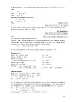
will be illuminated. But prior to this a simple application will show the ease of use.
A
mass is suspended from

a
point
by
a
spring of natural length
a
and stiffness
k,
as shown in
Fig.
2.1.
The mass is constrained to move in a vertical plane in which
the gravitational field strength is
g.
Determine the equations of motion in terms
of the distance
r
from the support to the mass and the angle
0
which is the angle
the spring makes with
the
vertical through the support point.
22
Lagrange
S
equations
Fig.
2.1
The system has

two
degrees
of
freedom and rand
8,
which are independent, can
serve as generalized co-ordinates. The expression
for
kinetic energy is
and for potential energy, taking the horizontal through the support as the datum
for gravitational potential energy,
k
2
V
=
-mgrcos
0
+
-
(r-a)
2
so
Applying Lagrange's equation with
9,
=
r
we have
so
and

ax
-
mrb2
+
mgcos8
-
k(r
-
a)
dr
From equation
(2.1)
-(
d
ax
)-($)=e
dt
ar'
mf
-
mr0'
-
mgcos8
+
k(r
-
a)
=
0
(i)

The generalized force
Q,
=
0
because there is no externally applied radial force
that is not included
in
V.
Generalized co-ordinates
23
Taking
0
as the next generalized co-ordinate
a'p.
ae
-
=
mr26
so
and

a'
-
mgr
sin
0
ae
Thus the equation of motion in
0
is

2mn4
+
mr2e
-
mgr
sin
0
=
o
(ii)
The generalized force in this case would be a torque because the corresponding
generalized co-ordinate is an angle. Generalized forces
will
be discussed later in
more detail.
Dividing equation
(ii)
by
r
gives
2m~O
+
mrb
-
mgsin
0
=
o
(iia)
and rearranging equations

(i)
and
(ii)
leads to
'2
mgcos0
-
k(r
-
a)
=
m(r
-
re)
and
-mgsin
0
=
m(2r.e
+
re)
(iib)
which are the equations obtained directly from Newton's laws plus
a
knowledge
of
the components of acceleration in polar co-ordinates.
In
this example there is not much saving of labour except that there is no
requirement to know the components of acceleration, only the components of

velocity.
2.2
Generalized co-ordinates
A
set
of
generalized co-ordinates is one in which each co-ordinate is independent and the num-
ber
of
co-ordinates is just sufficient to specify completely the configuration
of
the system.
A
system
of
N
particles, each free to move in a three-dimensional space, will require
3N
co-
ordinates
to
specify the configuration.
If
Cartesian co-ordinates are used then the set could be
{XI
Yl
ZI
x2
Y2
22.

*
.
XN
YN
ZN)
or
tX1
xZ
x3
x4
x5
x6
*
.
.
xn-2
xn-/
xn>
where
n
=
3N.
24
Lagrange
S
equations
This
is an example of a set of generalized co-ordinates but other sets may be devised
involving different displacements or angles. It is conventional to designate these co-
ordinates

as
(41
q2
q3
q4
4s
46

*qn-2
qn-I
qn)
If there are constraints between the co-ordinates then the number of independent co-ordi-
nates will be reduced. In general if there are
r
equations of constraint then the number of
degrees
of
freedom
n
will be
3N
-
r.
For a particle constrained to move in the
xy
plane the
equation
of
constraint is
z

=
0.
If
two
particles are rigidly connected then the equation of
constraint will be
(x2
-
XJ2
+
63
-
y,)2
+
(22
-
z1>2
=
L2
That is, if one point is
known
then the other point must lie on the surface of a sphere of
radius
L.
If
x1
=
y,
=
z,

=
0
then the constraint equation simplifies to
Differentiating we obtain
2x2
dx2
+
2y2 dy2
4
2.7,
dz2
=
0
This is a perfect differential equation and can obviously be integrated to form the constraint
equation. In some circumstances there exist constraints which appear in differential form
and cannot be integrated; one such example of a rolling wheel will
be
considered later.
A
system for which all tbe constraint equations can be written in the fomf(q,.
.
.qn)
=
con-
stant or a
known
function of time is referred to as
holonomic
and for those which cannot it
is

called
non-holonomic.
If the constraints are moving or the reference axes are moving then time will appear
explicitly in the equations for the Lagrangian. Such systems are called
rheonomous
and
those where time does not appear explicitly are called
scleronomous.
Initially we will consider a holonomic system (rheonomous or scleronomous)
so
that the
Cartesian co-ordinates can be expressed in the form
(2.2)
Xl
=
x,
(41
q2
* *
f
qrtt)
By the rules for partial differentiation the differential of equation (2.2) with respect to time is
so
thus
dt
at2
Differentiating equation
(2.3)
directly gives
Proof

of
Lagrange
S
equations 25
and comparing equation (2.5) with equation (2.6), noting that
vi
=
xi,
we see that
aii
-
axi

-
aqj
aqj
a process sometimes referred to as the cancellation of the dots.
From equation (2.2) we may write
hi
=
x$dqj
+
-dt
ax,
at
i
Since, by definition, virtual displacements are made with time constant
These relationships will be used in the proof of Lagrange’s equations.
2.3
Proof

of
Lagrange‘s equations
The proof
starts
with D’Alembert’s principle which, it will be remembered, is an extension
of the principle
of
virtual work to dynamic systems. D’Alembert’s equation for a system
of
Nparticles is
2
(F
-
rnliy6r;
=
0
1
SiSN
(2.10)
I
where
6r;
is any virtual displacement, consistent with the constraints, made with time fixed.
(2.1 1)
Writing
r,
=
x,i
+
xzj

+
x,k
etc. equation (2.10) may be written in the form
(6
-
rnlxl)6xl
=
0
1
SiSn
=
3N
1
Using equation (2.9) and changing the order of summation, the
first
summation in equation
(2.1 1
)
becomes
the virtual work done by the forces. Now
W
=
W(qj)
so
(2.12)
(2.13)
and by comparison of the coefficients
of
6q
in equations (2.12) and (2.13) we see that

(2.14)
This term is designated
Q,
and is known
as
a generalized force. The dimensions
of
this quan-
tity need not be those of force but the product of the generalized force and
the
associated
generalized co-ordinate must be that of work. In most cases this reduces to force and dis-
placement or torque and angle. Thus we may write
6W
=E
Q$qj
j
(2.15)
26
Lagrange's equations
In a large number of problems the force can be derived from a position-dependent poten-
tial
V,
in which case
e.=
av
*,
Equation (2.13) may now be written
where
Qj

now only applies to forces not derived
from
a potential.
Now the second summation term in equation (2.1 1) is
or, changing the order of summation,
(2.16)
(2.17)
(2.18)
We now seek a form for the right hand side of equation (2.18) involving the kinetic energy
of
the system in terms
of
the generalized co-ordinates.
The kinetic energy of the system of
N
particles is
Thus
because the dots may be cancelled,see equation (2.7). Differentiating wLrespect to time gives
but
so
Substitution of equation (2.19) into equation (2.18) gives
m,f,
ax,
=E[-
d
(-)
aT
-
"1
6qj

i
dt
aqi
I
(2.19)
(2.20)
Substituting from equations (2.17) and (2.20) into equation 2.1
1
leads to
The
dissipation
function
27
I
Because the
q
are independent we can choose
i3qj
to be non-zero whilst all the other
Sq
are
zero.
So
Alternatively since Vis taken not to be a function of the generalized velocities we can write
the above equation in
terms
of the Lagrangian
‘f
=
T

-
V
(2.2
1)
In the above analysis we have taken
n
to be
3N
but if we have
r
holonomic equations
of
constraint then
n
=
3N
-
r.
In practice it is usual to write expressions for
T
and Vdirectly
in terms of the reduced number of generalized co-ordinates. Further, the forces associated
with workless constraints need not be included in the analysis.
For example, if a rigid body is constrained to move in a vertical plane with they axis ver-
tically upwards then
.2
T
=
1If
(xi

+
$)
+
’.
8
and
V
=
mgy,
2 2
The constraint equations are fully covered by the use of total mass and moment of inertia
and the suppression
of
the z, co-ordinate.
2.4
The
dissipation function
If there are forces of a viscous nature that depend linearly on velocity then the force is given
by
F,
=-Xc,X,
/
where
c,
are constants.
The power dissipated is
P
=
cF,x,
P

=
XQ,q,
Q,
=
-XCy
4,
I
In terms of generalized forces
and
J
where
C,
are related to
e,,
(the exact relationship does not concern us at this point).
The power dissipated is
P
=
-XQJ4,
By
differentiation
28
Lagrange’s
equations
If we now define
$
=
PI2
then
af

=
-ei
aqi
(2.22)
The term
jF
is
known
as
Rayleigh
5
dissipative function
and is half the rate at which power
is being dissipated.
Lagrange’s equations are now
“(E)
dt
a$
-
(g)
+
$
=
Q.
J
(2.23)
where
Qj
is the generalized force not obtained
from

a position-dependent potential
or
a
dissipative function.
EXAMPLE
For the system shown in Fig. 2.2 the scalar functions are
k,
2
k2
Y
=
-XI
+
-(x2
-
XJ2
2 2
Ci
-2
C2
2 2
3
=
-XI
+
-(X2
-
X,f
The virtual work done by the external forces is
6W

=
F,
6x,
+
F,
6x,
For the generalized co-ordinate
x,
application
of
Lagrange’s equation leads
to
m,x,
+
k,x1
-
k2(x2
-
XI)
+
c,X,
-
~2(X2
-
XI)
=
F,
and for
x,
mg2

+
k2(x2
-
xI)
+
c2(X2
-
X,)
=
F2
Fig.
2.2
Kinetic enew
29
Alternatively we could have used co-ordinates
y,
and
y2
in which case the appro-
priate functions are
and the virtual work is
6W
=
F,6y,
+
F&YI
+
Y2)
=
VI

+
F2PYI
+
F26Y2
Application of Lagrange‘s equation leads this time to
m&
+
m,(y,
+
j2)
+
k,yl
+
ciI
=
fi
+
4
mz(Y1
+
Y2)
+
+
c2Y2
=
4
Note that in the first case the kinetic energy has no term which involves products
like
(iicjj
whereas in the second case

it
does. The reverse is true for the potential
energy regarding terms like
9;qj.
Therefore the coupling of co-ordinates depends on
the choice of co-ordinates and de-coupling in the kinetic energy does not imply that
de-coupling occurs in the potential energy.
It
can be proved, however, that there
exists
a
set of co-ordinates which leads to uncoupled co-ordinates in both the
kinetic energy and the potential energy; these are known as principal co-ordinates.
2.5
Kinetic
energy
The
kinetic
energy
of
a
system
is
T
=
L
miif
=
1
(ilT[m](i)

2
where
T
(1)
=
(XI
X2
.
*
X3N)
and
30
Lagrange
S
equations
We shall, in this section, use the notation
(
)
to mean a column matrix and
[
]
to indicate a
square matrix. Thus with
T
(X)
=
(XI
X,
.
. .

X*)
(4
=
[A1(4)
+
(b)
then we may write
where
and
Hence we may write
=
1(4>'
[AIT [ml [AI
(4)
+
(b)T[ml [AI
(4)
+
[ml
(b)
(2.24)
Note that use has been made of the fact that
[m]
is symmetrical. This fact also means that
[AI~[~][AI
is symmetrical.
T
=
T,
+

TI
+
To
2
Let us write the kinetic energy as
where
T,,
the first term of equation (2.24), is a quadratic in
q
and does not contain time
explicitly.
TI
is linear in
q
and the coefficients contain time explicitly.
To
contains time but
is independent
of
q.
If the system
is
scleronomic with no moving constraints or moving axes
then
TI
=
0
and
To
=

0.
T2
has the form
-
T
=
a,
4,G$
a,
-
a,,
=m
T,
=
Icai2
2rl
2
and in some cases terms like
q&
are absent and
T,
reduces to
2,
"
Here the co-ordinates are said to be orthogonal with respect to the kinetic energy.
Conservation laws
3
1
2.6
Conservation laws

We shall now consider systems for which the forces are only those derivable
from
a
position-dependent potential
so
that Lagrange’s equations are of the form
A(%)
dt
aS,
-
(2)
=
0
A(%)
=
0
If a co-ordinate does not appear explicitly in the Lagrangian but only occurs
as
its time
derivative then
dt
%I
Therefore
aq1
-
a
=
constant
In this case
q,

is said to be a cyclic or ignorable co-ordinate.
Consider now a group
of
particles such that the forces depend only on the relative posi-
tions and motion between the particles. If we choose Cartesian co-ordinates relative to an
arbitrary set of axes which are drifting in the
x
direction relative to an inertial set
of
axes
as
seen in Fig.
2.3,
the Lagrangian is
1
-2
1
t=N1
91
=
E
z
112,
(X+
XI?
+
y;
+
z,
-

V(x,
y,
z,)
I=
I
Because
X
does not appear explicitly and is therefore ignorable
r=N
2%
=
crn,.(X
+
x,)
=
constant
ax
I=I
If
X+
0
then
(2.25)
r=N
.
,=I
I:
m,x,
=
constant

Fig.
2.3
32
Lagrange
S
equations
This may be interpreted as consistent with the Lagrangian being independent
of
the position
in space of the axes and this also leads to the linear momentum in the arbitrary
x
direction
being constant or conserved.
Consider now the same system but this time referred to an arbitrary set
of
cylindrical co-
ordinates. This time we shall superimpose a rotational drift
of
r
of the axes about the
z
axis,
see
Fig.
2.4.
Now the Lagrangian is
x
=
z
-L

r,
(e,
+
r)*
+
if
+
Z,
-
v(rl,el,zl)
12
m[2.
.'I
Because
y
is a cyclic co-ordinate
az
2'
-,-
=
Cm,r,(O,
+
y)
=
constant
aY
I
If we now consider
y
to tend to zero then

-,-
ax
=
~mlr~bl
=
constant
aY
1
(2.26)
This implies that the conservation of the moment of momentum about the
z
axis is associ-
ated with the independence
of
aXldr
to a change in angular position
of
the
axes.
Both the above show that
aXla4
is related to a momentum or moment of momentum. We
now define
aZ/aq,
=
p,
to be the
generalized momentum,
the dimensions of which will
depend

on
the choice of generalized co-ordinate.
Consider the total time differential of the Lagrangian
-
a=
xpqJ+xTa
ax-
6%
+-
ap
(2.27)
dt
J
aqJ
J
a%
at
d
ax
If all the generalized forces,
QJ,
are zero then Lagrange's equation is
-(
dt
as,
)-(?)=O
Substitution into equation
(2.27)
gives
Fig.

2.4
Hamilton
's
equations
33
ax ax
Thus
d
dt
at
-
.)
=

ax
i
and if the Lagrangian does not depend explicitly on time then
-
z
=
constant
i
as,
(2.28)
(2.29)
Under these conditions
Z
=
T
-

V
=
T,(qjqj)
-
V(qj).
Now
1
2ii
&
=
-
ZZa,qi&,
a,
=
aji
so
because
aii
=
aii.
We can now write
so
that
T$qj
-
9;
=
2T2
-
(T,

-
V)
=T,+V=T+V
=E
the total energy.
From equation
(2.29)
we see that the quantity conserved when there are (a) no general-
ized forces and (b) the Lagrangian does not contain time explicitly is the total energy.
Thus
conservation of energy is a direct consequence of the Lagrangian being independent of time.
This
is
often referred to
as
symmetry in time because time could in fact be reversed without
affecting the equations. Similarly we have seen that symmetry with respect to displacement
in space yields the conservation of momentum theorems.
2.7
Hamilton's
equations
The quantity between the parentheses in equation
(2.28)
is
known
as
the
Hamiltonian H
or in terms of momenta
(2.30)

(2.3
1)