Advanced Engineering Dynamics 2010 Part 12 pdf
Bạn đang xem bản rút gọn của tài liệu. Xem và tải ngay bản đầy đủ của tài liệu tại đây (595.54 KB, 20 trang )
2
14
Robot
ann
dynamics
A14
=
a,
COS
O4
+
d6
COS
e4
Sin
8,
A,,
=
sin
8,
cos
e5
cos
8,
-
cos
e4
sin
8,
Azz
=
-sin
O4
cos
8,
sin
8,
-
cos
8,
cos
8,
A23
=
sin
O4
sin
8,
A24
=
a4
sin
O4
+
d,
sin
O4
sin
8,
A3,
=
sin
8,
cos
e6
A32
=
-sin
8,
sin
e6
A,,
=
-COS
8,
A34
=
-d6
COS
8,
A4,
=
0
A4*
=
0
A,,
=
0
A-
=
1
In this example the end effector is shown in a position for which
8,
=
90",
8,
=
90"
and
O6
=
0.
The complete transformation from the
(~2)~
axes to the
(xyz),
set of axes is
3[A16($)6
($10
=
0[A16(d)6
=
o[A13
or, in general terms,
(8.30)
It is seen by putting
x6
=
0,
y6
=
0
and
z6
=
0
that
(ry,rz)
is the location of the origin of the
(Vz)6
axes. If we put
x6
=
I
with
y6
=
o
and
z6
=
o
we have
x,
-
rx
=
n,
Yo
-
yv
=
nv
z,,
-
r,
=
n,
Therefore
(n,n,n,)
are the direction cosines of the
x6
axis. Similarly the components of
(s)
are the direction cosines of the
y6
axis and the components of
(a)
are the direction cosines
of the
z6
axis. These directions are referred to as normal, sliding and approach respectively,
the sliding axis being the gripping direction.
8.3.13
THE INVERSE KINEMATIC PROBLEM
For the simpler cases the inverse case can be solved by geometric means,
see
equations
(8.1)
to
(8.3);
that is, the joint variables may be expressed directly in terms ofthe co-ordinates and
ori-
Kinematics
of
a
robot
ann
2
15
entation of the end effector. For more complicated cases approximate techniques may be used.
An
iterative method which
is
found to converge satisfactorily is first to locate the end effec-
tor by a trial and error approach to the first three joint variables followed by a similar method
on the last three variables for the orientation of the end effector. Further adjustments of the
position of the
arm
will be necessary because moving the end effector will alter the refer-
ence point.
This
adjustment will then have a small effect upon the orientation.
Small variations of the joint variables can be expressed in terms of small variations of the
co-ordinates. For example, if
(p)
is a function of
(e)
then
or
ae,
ae,
ae,
(8.3
1)
where
[D]
is the matrix
of
partial differential coefficients which are dependent
on
position.
It is referred to by some authors as the Jacobian. The partial differential coefficients can be
obtained by differentiation
of
the respective
A
matrices. The matrix, if not singular, can be
inverted to give
(W
=
[DI-'
@PI0
(8.32)
since
(Ae)
=
(e)n+l
-
(01,
(e)n+l
=
(e),
+
[DI,'
(~~10
(8.33)
Repeated use enables the joint positions to be evaluated.
In general since
(PI0
=
,[AI,
*
.
n-I[Aln
(@In
then
where qi is one
of
the variables, that is
0
or
d.
for
a
revolute joint or of
di
for a prismatic/sliding joint.
It should be noted that in this context
(p),,
is constant and that
i-,[A]i
is a finction of
Bi
For the general case
;-,[AI;
=
SO,
CB;Ca, -CBiSai
aisei
Sai
Cui
0 0
1
;-,[AI;
=
1
cei
-SeiCai
SB,Sa,
aiCei
SO,
CB;Ca,
-CBiSai
aisei
0
Sai
Cui
0 0
0
1
so
differentiating with respect to
Oi
2
16
Robot
arm
dynamics
1
1
-SO,
-CB,Ca,
CB,Sa, -a,SB,
CB, -SB,Ca,
SB,Sa, a,CB,
0
0
0
0
0
0
0 0
CB, -S0,Ca,
SB,Sa, a,CB,
SO,
C0,Ca,
-CB,Sa, a,SB,
a
30,
,-i[AI,
=
-
Note that the right hand side of equation (8.34) may be written
Ca,
dl
0 0 0
1
or
in symbol form
a
80,
,-i[AI,
=
[Ql
,-i[Al,
-
where
In a similar manner
(8.34)
(8.35)
(8.36)
where
0000
[I::::]
0001
8.3.14
The basis
for
determining the joint velocities given the motion of a particular point has
already been established in section 8.3.13 where the
matrix
[D]
was discussed.
If
we con-
sider the variations to take place in time
At
and then make
At
+
0
then,
by
definition
of
velocity,
(do
=
[Dl(e)
(8.37)
LINEAR
AND
ANGULAR VELOCITY
OF
A
LINK
so
the
joint velocities can found
by
inversion
<e>
=
[DI-'(P)o
(8.38)
Kinematics
of
a
robot
ann
2
17
Refemng to Fig.
8.20
we can also write
($10
=
o[Aln(d)n
Thus
(8.39)
d
dt
-
($10
=
0[21n(~)n
where
($)n
is constant.
Consider the product of two
A
matrices
[
::;’
(:,,I
[
‘1
(,,;I
=
[
[RI;;],
1
[RlI(u:,
+
(41
]
It is readily seen that for any number
of
multiplications the top left submatrix will
be the product
of
all the rotation matrices and the top right submatrix
is
a func-
tion of
[R]
and
(u)
submatrices. So in general the product of
A
matrices is of the
form
[RI
(r)
[A1
=
LO)
1
1
We have already shown that the column matrix
(r)
is the position of the origin of the final
set
of
axes
and
the three columns of
[R]
are the direction cosines
of
these axes.
So
(p)o
=
[R](p),
+
(r)
and the position
of
a point relative to the base axes is
(ph
-
(r)
=
(AP)
=
[RI(p)n
Differentiating with respect to time gives the relative velocity
(AP)
=
[RI(P)~
(8.40)
Fig.
8.20
2
18
Robot
arm
dynamics
so
it is seen that
[i]
is related to the angular velocity of the nth link. Now
(Ab)
is the veloc-
ity of
P
relative to
0,
referred to the fixed base axes. We can find the components referred
to the
(xyz),
axes by premultiplying
(AP)
by
[RI-’
=
[RIT
thus
(8.4
1)
We know that
[RIT[R]
=
[I]
so
by differentiating with respect to time we have
[R],T[i]
+
[iIT[R]
=
[O]
and as the second term is the transpose of the first it follows that
[R]
[R]
is
a skew symmetric matrix. This matrix will have the form
(Ab),
=
[RI~(A~)
=
[RI~[RI(P)~
where
(a,ra,a,)T
is the angular velocity vector of the nth link.
Now
i=n
[Rln
=
GI
[Rli
so
101;
=
[RlT,[Rln
=
[RIT,
2
[Rll[R12
*
[Ql[Rli
[Rlnqi
where
(8.42)
0
-1
0
[.I=[
01
for the
3
X
3
rotation matrices. Each term in the above series is equivalent to the change
in
[a]’
as we progress from link to link.
8.3.15
LINEAR AND ANGULAR ACCELERATION
The second differentiation can be found by simply reapplying the rules developed for the
first differentiation with respect to time.
We see that since
(b)o
=
0[4n(b)n
(8.43)
In order to see the operation let
us
look at a two-dimensional case and with
n
=
2, as
shown in Fig. 8.21, for which theA matrices are functions of
8’
and
8,
so
that
(810
=
0[4l
I[42(b)2
where
Kinematics
of
a
robot
arm
2
19
Fig.
8.21
and the
A
matrix for the two-dimensional case (for which
a
=
0)
may be written
I
lo
0
1
cos
8
-sin
8
a
cos
8
[A]
=
sin
8
cos
8
a
sin
8
Therefore
(P>o
=
[Qlo[Ali
i[Al2
9i<P>2
+
o[Ali[Qli[Al2
e2(P)2
and
(P>o
=
[QloZ[Ali
i[Alz
ef(P12
+
[QIo[~li[QI~[~l~
eie2(P>2
+
[Qlo[Ali
iW12
4i(P)2
+
[Qlo[~li[Qli[~lt
eie2(P>2
+
o[Ali[Ql~[Al2
e,’(P>2
+
o[~li[Qli[~l2
GI($),
If we require the origin of the
(x
Y)~
axes to follow a specified path then for each point on
the path,
(x
Y)~,
the corresponding values
of
8,
and
O2
can be found.
Also
if the velocities and
accelerations of the point are prescribed the derivatives
of
the angles can be calculated using
the above equations.
Once the values of
e,,
8,
and their derivatives are known any linear or
angular
velocity
and linear or angular acceleration can be found.
The above scheme can in principle readily be extended to the three-dimensional case and
any number of links can be considered.
The general form of the equations is
i=n
(PI0
=
!i
i-i[Ali(P)n
=
[Wn(P)n
(8.44)
where
[un
is defined by the above equation
(8.44).
220
Robot
arm
dynamics
The velocity is
where
[Uln,i
is a fimction of the
A
matrices
and
hence of the joint variables, that is
[Uln.i=
,[All
.
.
[Qli-~[Ali
. .
*
,[AI, (8.46)
For the acceleration
I=
I
where
(8.47)
(8.48)
We have shown previously that in general
so
[R]
(r)
[AI=[
]
Since, for constant
(p),,,
we have
tb)
=
[jl<i>n
then we have
(PI
=
[RI(P)~
+
('1
and
thus the acceleration of
P
relative to the origin of the
(vz),
axes,
(Ap),,
=
(p)
-
(P)
=
[RI(P)~*
If we now refer the components of this vector
to
the
(vz),
axes we have
[~l'(~ii)n
=
[RI~[~I(P)~.
[0IX
=
[R]'[d]
Now
so
[&IX
=
[R]'[R]
+
[RIT[k]
[R]'[k]
=
[&I"
-
[ri]'[ri]
and
therefore
Kinematics
of
a
robot
am
22
1
Also
[RIT[il
=
[ilT([~l[RIT)
[il
=
([~lT~~l)T([~lT~~l)
=
[o]xT[o]x
=
-[o]"[o]"
Finally
[RI~(AP)~
=
[RI~[RI(P)~
=
{[&Ix
+
[oIX[~Ix)(p)n
=
[bI"(p)n
+
[oI"[~I"(p)n
(8.49)
where
(p),
is of constant magnitude. This result is seen to agree with that obtained from
direct vector analysis
as
shown in the next section.
8.3.16 DIRECT VECTOR ANALYSIS
It is possible to derive expressions for the velocity and acceleration of each
link
by vector
analysis. The computation in this case uses only
3
x
1
and
3
x
3
matrices rather than the
full
4
X
4
A
matrices used in the last section.
Referring to Fig.
8.22
we see that the position vector of the origin
of
the
(xyz),
axes is
r,
=
r,-,
+
d,
+
0,
(8.50)
Fig.
822
222
Robot
arm
dynamics
and
The velocity of
0
is
dr,
dri-l
dt dt
+
-
(d,
+
a;)
+
0,
x
(dj
+
ai)
at
Vi=-=-
(8.51)
(8.52)
We require
our
reference axes to be fixed to the ith link in order that when the moment of
inertia of the ith link is introduced it shall be constant. For the second term on the right the
partial differentiation means that only changes in magnitude
as
seen from the
(qz),
axes are
to be considered. For a revolute joint where both
d
and
u
are constant in magnitude this term
will be zero. For a prismatic joint the term will be
Aiki-,.
To simplify the appearance of the subsequent equations we again use
ui
=
dj
+
ai
(8.53)
and write
vi-,
for d(r,-,)/(dt)
so
equation
(8.52)
becomes
au,
at
v.
=
v.
+
-
+
0;
x
ui
1
1-1
For a revolute joint the second term on the right hand side is zero.
The acceleration of
0;
is
(8.54)
(8.55)
For a revolute joint the second and fourth terms on the right hand side are zero whilst for a
prismatic joint the third term is zero.
Both of these equations may be expressed in matrix form assuming that the base vectors
for all terms are the unit vectors of the
(qz),
axes.
Thus
we may write
aL,
aO,
au,
at2
at
at
u,
=
tZ-1
+
-
+
-
x
u,
+
0,
x
-
+
0,
x
(0,
x
u,)
(8.56)
a
at
(VI,
=
(a,
+
-
(41
+
Lo]:
(41
and
a2
a
a
at
at
at
(a),
=
(a),-,
+
7
W,
+
(
-
[a]:
)
W,
+
[a]:
-
(u),
+
[o~:[ol:(u),
(8.57)
where
a
[a]:
=
[R]:[R],
and
-[a]:
=
[R]T[d],
+
[R]f[k],
at
also
[RI,
=
[RI~
.
*
[QI[RI,
*
*
[~~nii
and
[k],
=
[R],
. .
.
[Q][RIj
.
.
.
[R],9,
+
C
C
[R],
.
[Q][R],
. .
.
[Q][R],
.
[R],eiij
i=n
j=n
,=I
j=l
Kinetics
of
a
robot
am
223
8.3.17
TRAJECTORY
PLANNING
AND CONTROL
In a practical pick and place
type
of operation an object is to be moved from point A to
point
B
and, for example, has to avoid an obstacle
C,
as indicated in Fig.
8.23.
The problem
is often tackled by planning for the end effector to move from A to
B
so
as
to arrive with
low speed at
B
and then to align the gripper. The exact path
is
not important apart from the
three specified points,
so
there are an infinite number of possible paths that the
arm
can fol-
low. The many factors which affect the choice of path are outside the scope of this book
as
we are concerned only with the pure dynamics of the problem.
One technique used is to consider the path to be constructed from short segments passing
through
a number of prescribed points. Usually a polynomial of third or fourth order is cho-
sen to represent the path between the specified points.
Another powexfbl method is to use position sensors to give feedback to an automatic
control system. These control systems are frequently digital, which makes adaptive control
easier.
Fig.
8.23
8.4
Kinetics
of
a robot arm
Our next task is to determine the forces and couples associated with the prescribed motion.
In the practical case it is not always possible to generate the required forces
so
the motion
which ensues from given forces may need to be calculated.
A dynamical model may be used for the prediction of performance or for forming part of
a real-time control algorithm.
We shall use Lagrange’s equation in conjunction with homogeneous transformation
matrices and the Newtoe-Euler approach using a vector algebra method. It should be noted
that both Lagrange and Newton-Euler could be associated with either the homogeneous
matrix formulation or vector algebra.
8.4.1
LAGRANGE’S EQUATIONS
Here we only generate one equation for each degree of freedom of the system and the basic
formulation only needs expressions for velocities and not for acceleration. However, differ-
entiation of the velocity- and position-dependent functions is required.
224
Robot
arm dynamics
Thus the kinetic energy of link
n
will be
(8.58)
where
R
is the number of point masses used to represent the rigid body. For an exact repre-
sentation
R
2
3.
The total kinetic energy will be just the sum of the energies for each link in the chain.
It would be convenient to be able to reverse the order of summation since
(jjr),,
and
mr
are
properties
of
the link and do not depend on its location.
This
can be achieved by noting that
Xofo
'fqo
To<o
0
Trace
($),(pi
=
Trace
1:'
zoxo
-?$
y:
ZGO
i
]
.2
=
i;
+
yo
+
i;
(8.59)
2
=
vo
So
we may now write
(8.60)
The link variables,
8
or
d,
satisfy the requirements for generalized co-ordinates and
so
will be designated by
q,
as
is usual in Lagrange's equations. Also the centre term depicts the
inertia properties of the nth link and will be abbreviated to+[J],. Note that
[J],
is a
sym-
metric matrix. The top left 3 x3 submatrix
is
related to the moment
of
inertia matrix
of
the
nth link relative to the nth joint, but is not identical to it. Thus
Cmy2 Cmyz
Cmzr
Cmzy
Cmz'
Cmy Cmz
Emz
In
terms
of
[J]
the
kinetic energy of the
nth
link
is
Kinetics
of
a
robot
ann
225
We now need to carry out the differentiations
as
prescribed by Lagrange's equations,
but since the second term is the transpose of the first
Therefore
In a similar manner we can obtain
(8.61)
(8.62)
So
for the nth link
We are now in a position to sum over the whole arm of
N
links. For clarity the constant
terms are now taken to the right of the summation sign to give
=
Qk
(8.64)
the generalised force, where
T
=
ET.
For revolute joints
Q
will be the torque at the pivot and for a prismatic joint
Q
will be the
sliding force.
Equation
(8.64)
may be written in a more compact form by reversing the order of
sum-
mation. This requires adjusting the limits. The form given below can be justified by expan-
sion. The term max(ij,k) means the highest value
of
i,j,
or
k
(8.65)
226
Robot
ann dynamics
where
(8.66)
(8.67)
8.4.2 NEWTON-EULER METHOD
This method will involve all internal forces between each link
as
indicated
on
a free-body
diagram, as shown in Fig. 8.24. Expressions for the accelerations of the individual centres
of mass and the angular velocities and accelerations can be found as discussed in the previ-
ous sections.
So
for each link, treated as a rigid body, the six equations of motion can be formulated.
With reference to Figs 8.22 and 8.24 the equations of motion for the ith link are
(8.68)
6
+
e-,
=
miuGi
and
(8.69)
d
dt
C;
+
Ci-l
+
rG;xI;;
-
(pi
-
rGi)
X&
=
-
(JGj’mj)
where
JGj
is the moment of inertia dyadic referred to the centre of mass of the ith link.
The acceleration of the centre of mass,
uGi
,
may be found from
(8.70)
a
at
acj
=
u;
+
-(O,)X
rGi
+
O,X(O;X
rGi)
Discussion
example
227
Fig.
8.24
The above three equations
may
also be written
in
matrix form using
(xyz),
axes as the
(F)i
+
(R,-=
4(a)Gf
(8.71)
basis
(C),
+
(Q-I
+
(.>1;,(F),
-
[(PI,
-
(T)GIIX(F)I-I
=
[JlG,;jT
a
(01,
+
[JIG,
[~l:<w,
(8.72)
WG,
=
(4,
+
$4x(%I
a
+
[~l:~~l:(~lG,
(8.73)
Discussion
example
A
spherical robot is shown in Fig. 8.25(a). During operation the position co-ordinates are:
8,
=
90",
0,
=
60"
and
d,
=
0.8
m.
Also
d0,ldt
=
2radls constant and dd,ldt
=
3ds
constant.
The inertial data are
for link 2: mass
=
20kg moment of inertia about
G,
=
8kgm'
for
link
3:
mass
=
lOkg moment of inertia about G,,
=
4kgm2
a) Using the
A
matrices calculate the position and velocity
of
the end of the
arm
E.
b) Using Lagrange's equation obtain the equations of motion for co-ordinates
0,
and
d,.
(a) The table of link parameters is first constructed. Referring to Fig. 8.25(a) the origin of
the
(xyz),
axes has been chosen to coincide with the origin of the
(xyz),
axes. By using the
data sheet given at the end of the chapter we see that as
a
is the distance between successive
z axes all the
a
dimensions are zero.
OG,
=
0.2m and
G,E
=
0.3m (see Fig.
8.26)
The distance between successive
x
axes is
d
and hence
d,
=
0.
228
Robot
ann
dynamics
(4
Fig.
8.25
(a)
and
(b)
Now
a
is the rotation of one
z
axis relative to the previous
z
axis
so
aI
=
-90"
and
a,
=
The table is
as
follows:
90".
Special care
is
needed to ensure that the signs are correct.
Link
e
a
a
d
1
90
'
-90'
0
D,
=O
2
60
'
90"
0
0
3
0
0
0
0.8
With reference
to
the data sheet the three
A
matrices are
ce,
o
sel
o
&41,=[;
;l
9'
;]
Discussion
example
229
The
ce,
o
se,
se,
o
-ce2
1
0
0 00
0
0
l[42
=
I
overall transformation matrix is
0
:I
1
:j
1
d3
,[TI3
=
oPI3
=
o[A]i 1[Al2 ,[AI3
1
ce,ce,
se,
ce,se,
d3ce,se2
se,ce,
-ce,
se,se,
d3se,se,
-
se,
0
Cf-32
d3C02
0
0 0
1
=
[
(;I
(3)
(a)
(P)]
00
1
=I
Here the last column gives the co-ordinates
of
the
(~yz)~
axes
xE0
=
d3cos(8,)sin(8,)
=
0
yEO
=
d3sin(8,)sin(8,)
=
0.8
X
1
X
0.866m
zEO
=
d3
COS(
8,)
=
0.8
x
0.5m
These results can easily be verified by simple trigonometry.
We shall now use the
A
matrices to evaluate the velocity of the point
E.
Now
d
(pE)o
=
dt
O[A]~(PE)~
=
o[Al3 @~)3
There is only one term on the right hand side of the equation because the position vector of
point
E
as seen from
the
(xyz),
axes is
(0
o o
llT for all time.
For brevity let us write ,[A],
=
AIA2A3
so,
with reference to equations
(8.35)
and
(8.36)
we have
0[i]3
=
QA,A2A3i),
+
A,QA,A,i),
+
A,A,P!3Li,
As
4,
=
0
the
first
term is zero and by direct multiplication the other
two
terms are
I
0 0
0
-0.866
0
0.5
-0.500
0
-0.866
-0.779
0
0
0 0
I
230
Robot
arm
dynamics
0 0 0
0
1
0
0
0.866
0
0.500
A,A2PA3d3
=
1
i
o
0
0 0
0
The velocity
of
E
is given by summing the last columns
of
the preceding
two
matrices
XEO
=
0
YE0
=
0.4~2
+
0.866~3
=
3.398d~
2,
=
-0.693~2
+
0.500~3
=
-0.114d~
Again these results are readily confirmed by direct means.
convenient mathematical computer package.
(b) Lagrange’s equations are
The matrix multiplications involved in the above calculations can be carried out using any
aT
av
d4
(;:)
-
G
+
a41
=
Qi
The virtual work done by the active forces and couples is
~FV
=
Q16qi
+
Q26q2
6W
=
C260,
+
F36d3
where
C,
is the torque about the
zo
axis acting on link
2
and
F3
is the force acting on link
3
along the
Z,
axis.
The kinetic energy
(see
Fig.
8.26)
is
T
=
-
m,(a6)’
+
124
+
m3[(d3
-
b),g
+
ai]
+
13%
2
l{
.,I
For
qi
=
8,
aT
=
[rn2a2
+
1,
+
I~
+
m,[(d3
-
b12]i2
8%
-
=
[rn,
+
I*
+
I,
+
m3(d3
-
b)2~82
+
2m3(d3
-
b)i3&
dt
d
(aT)
ae,
Fig.
8.26
Discussion
example 23
1
ar
-
av
-
-0,
-
=O
and
Q=C2
(302 a02
[m2
+
I,
+
1,
+
m3(d3
-
bf38,
+
2m3(d3
-
b)d3g2
=
C2
so
the equation of motion for
e2
is
Inserting the numerical values gives
and
as
0,
=
0,
d,
=
3ds
and
&
=
2radls
we have
(15.3)6,
+
loci3&
=
c2
C2
=
60Nm
Similarly for
qi
=
d3
L(x)
=
m3d3
and
-
aT
=
m3(d3
-
b)0,
‘2
dt
ad,
ad3
so
the equation of motion for d3
is
m3d3
-
m3(d3
-
b)e:
=
4
The same set of equations can be formed using
D’
Alembert’s principle. We refer to Fig.
8.27
where the accelerations have been determined by direct means. Also shown with heavy
arrows are the virtual displacements.
D’Alembert’s principle states that the virtual work done by the active forces less that done
by the ‘inertia forces’ equals zero.
For virtual displacement
65
=
60,’
(6d3
=
0)
C260,
-
126,60,
-
m2a6,a60,
-
m3[(d3
-
b)8,
+
2a,0,](d3
-
b)68,
-
1~6~~0,
=
o
and now with
65
=
ad,,
(68,
=
0)
F,M,
+
m3[(d3
-
b)e:
-
d3]6d3
=
o
Thus
C,
-
[I,
+
r3
+
m2a2
+
m3
(d3
-
b)’16,
-
2m,ci,B,(d3
-
b)
=
o
Fig.
8.27
232
Robot
arm
dynamics
and
F,
+
m3[(4
-
b)G2
-
d3]
=
0
Let
us
now return to the Lagrange method but this time make use of the 4x4 homoge-
neous matrix methods. Using equation
(8.65)
we have
N
=
3
but since link
1
is stationary
it is not involved in the kinetics, although it still affects the geometry.
The inertia data is not in the form needed to generate the [J] matrices. If we define
I,
=
Em2
+
Emy2
+
Emz2 then it
is
easy to show that 21,
=
I,
+
I,
+
I,.
Therefore
2
cmx
=
I,
-
z,
cy2
=
Ip
-
IF
cz2
=
I,
-
I,
For link 2 we use the parallel axes theorem to to evaluate
I,
=
ZGv
+
m2a2
=
8.0
+
20 ~0.2~
=
8.8
kgm2. We will assume that
Zox
=
Z,
and that
Zoz
is negli ible. Therefore
Z,
=
8.8
kgm2.
It now follows that
Xmx2
=
0,
Emy2
=
0
and
Ern2
=
8.8kgm. The term
Xmz
=
20x0.2
=
4.
P
The inertia matrix for link 2 is
0
0
[J12
=
()
I
0
similarly for link
3
0
0
8.8
4
0
0
4.9
-3
4
20
:I
-3
10
Ej
Robotics data sheet
233
All other terms are zero. Thus
15.38,
+
5.00,d3
=
C,
In this problem the geometry is particularly simple
so
that the 4x4 matrix methods can
It is left as an exercise for the reader to obtain the equations of motion using the New-
readily be compared with other methods.
tonian approach. The free-body diagrams and kinematics are shown in Fig.
8.28.
Fig.
8.28
Robotics data sheet
LINK
CO-ORDINATE
SYSTEM
The
z(i)
axis is the axis of rotation or sliding ofjoint
(i
+
1). The
x(i)
axis lies along the com-
mon normal to the
z(i)
and
z(i-
1) axes. This locates the origin of the
(xyz),
axes except when
the
z
axes are parallel; in this case choose the normal which passes through the origin of the
(xy~)~-,
axes.
e(i)
is the joint angle from the
x(i
-
1) axis to the
x(i)
axis about the
z(i
-
1) axis.
d(i)
is the distance from the origin of the
(i-
1)
co-ordinate frame to the intersection of the
a(i)
is the offset distance from the intersection of the
z(i-
1) axis with the
x(i)
axis and the
a(i)
is the offset angle from the
z(i-
1) axis to the
z(i)
axis.
z(i-
1)
axis with the
x(i)
axis along the
z(i-
1)
axis.
z(i)
axis (i.e. the shortest distance between the
z(i-
1)
axis and the
z(i)
axis).