Dynamics of Mechanical Systems 2009 Part 4 docx

132 Dynamics of Mechanical Systems
where ωω
ωω
QP
and αα
αα
QP
are the angular velocity and angular acceleration, respectively, of the
connecting rod QP. Because QP has planar motion, we see from Figure 5.3.4 that ωω
ωω
QP
and
αα
αα
QP
may be expressed as:
(5.3.17)
where n
z
(= n
x
× n
y
) is perpendicular to the plane of motion. Also, the position vector QP
may be expressed as:
(5.3.18)
By carrying out the indicated operations of Eqs. (5.3.15) and (5.3.16) and by using Eqs.
(5.3.13) and (5.3.14), v
P
and a
P

become:
(5.3.19)
and
(5.3.20)
Observe from Figure 5.3.4 that P moves in translation in the n
x
direction. Therefore, the
velocity and acceleration of P may be expressed simply as:
(5.3.21)
where x is the distance OP. By comparing Eqs. (5.3.19) and (5.3.20) with (5.3.21), we have:
(5.3.22)
FIGURE 5.3.4
Geometrical parameters and unit vectors of the piston, connecting rod, and crank arm system.
Q
ᐉ
φ θ
r
O
n
n
n
n
y
θ
r
z
x
P n
x
ωωαα

QP z z
=− =−
˙˙˙
φφnnand
QP
QP n n=−llcos sinφφ
xy
vnn
Pxy
rr=− −
()
+−
()
ΩΩsin
˙
sin cos
˙
cosθφφ θφll
an
n
Px
y
r
r
=− − −
()
+− − +
()
Ω
Ω

22
22
cos
˙˙
sin
˙
cos
sin
˙˙
cos
˙
sin
θφφφ φ
θφ φφ φ
ll
ll
vn an
Px x
xx==
˙˙˙
and
P
˙
sin
˙
sinxr=− −Ωθφφl
0593_C05_fm Page 132 Monday, May 6, 2002 2:15 PM
Planar Motion of Rigid Bodies — Methods of Analysis 133
(5.3.23)
(5.3.24)

and
(5.3.25)
Observe further from Figure 5.3.4 that x may be expressed as:
(5.3.26)
and that from the law of sines we have:
(5.3.27)
By differentiating in Eqs. (5.3.26) and (5.3.27), we immediately obtain Eqs. (5.3.22) and
(5.3.23). Finally, observe that by differentiating in Eqs. (5.3.22) and (5.3.23) we obtain Eqs.
(5.3.24) and (5.3.25).
5.4 Instant Center, Points of Zero Velocity
If a point O of a body B with planar motion has zero velocity, then O is called a center of
zero velocity. If O has zero velocity throughout the motion of B, it is called a permanent
center of zero velocity. If O has zero velocity during only a part of the motion of B, or even
for only an instant during the motion of B, then O is called an instant center of zero velocity.
For example, if a body B undergoes pure rotation, then points on the axis of rotation
are permanent centers of zero velocity. If, however, B is in translation, then there are no
points of B with zero velocity. If B has general plane motion, there may or may not be
points of B with zero velocity. However, as we will see, if B has no centers of zero velocity
within itself, it is always possible to mathematically extend B to include such points. In
this latter context, bodies in translation are seen to have centers of zero velocity at infinity
(that is, infinitely far away).
The advantage, or utility, of knowing the location of a center of zero velocity can be
seen from Eq. (5.3.10):
(5.4.1)
where P and Q are points of a body B and where r locates P relative to Q. If Q is a center
of zero velocity, then v
Q
is zero and v
P
is simply:

(5.4.2)
0 =−rΩcos
˙
cosθφ φl
˙˙
cos
˙˙
sin
˙
cosxr=− − −Ω
22
θφφφ φll
0
22
=− − +rΩ sin
˙˙
cos
˙
sinθφ φφ φll
xr=+cos cosθφl
l
sin sinθφ
=
r
vv r
PQ
=+×ωω
vr
P
=×ωω

0593_C05_fm Page 133 Monday, May 6, 2002 2:15 PM
134 Dynamics of Mechanical Systems
This means that during the time that Q is a center of zero velocity, P moves in a circle
about Q. Indeed, during the time that Q is a center of zero velocity, B may be considered
to be in pure rotation about Q. Finally, observe in Eq. (5.4.2) that ω is normal to the plane
of motion. Hence, we have:
(5.4.3)
where the notation is defined by inspection.
If a body B is at rest, then every point of B is a center of zero velocity. If B is not at rest
but has planar motion, then at most one point of B, in a given plane of motion, is a center
of zero velocity.
To prove this last assertion, suppose B has two particles, say O and Q, with zero velocity.
Then, from Eq. (5.3.10), we have:
(5.4.4)
where r locates O relative to Q. If both O and Q have zero velocity then,
(5.4.5)
If O and Q are distinct particles, then r is not zero. Because ωω
ωω
is perpendicular to r, Eq.
(5.4.5) is then satisfied only if ωω
ωω
is zero. The body is then in translation and all points have
the same velocity. Therefore, because both O and Q are to have zero velocity, all points
have zero velocity, and the body is at rest — a contradiction to the assumption of a moving
body. That is, the only way that a body can have more than one center of zero velocity,
in a plane of motion, is when the body is at rest.
We can demonstrate these concepts by graphical construction. That is, we can show that
if a body has planar motion, then there exists a particle of the body (or of the mathematical
extension of the body) with zero velocity. We can also develop a graphical procedure for
finding the point.

To this end, consider the body B in general plane motion as depicted in Figure 5.4.1.
Let P and Q be two typical distinct particles of B. Then, if B has a center O of zero velocity,
P and Q may be considered to be moving in a circle about O. Suppose the velocities of P
and Q are represented by vectors, or line segments, as in Figure 5.4.2. Then, if P and Q
rotate about a center O of zero velocity, the velocity vectors of P and Q will be perpen-
dicular to lines through O and P and Q, as in Figure 5.4.3.
Observe that unless the velocities of P and Q are parallel, the lines through P and Q
perpendicular to these velocities will always intersect. Hence, with non-parallel velocities,
the center O of zero velocity always exists.
FIGURE 5.4.1
A body B in general plane motion.
FIGURE 5.4.2
Vector representations of the velocities of particles
P and Q.
vr
PPP
vr==ωω or ω
vv r
OQ
=+×ωω
ωω× =r 0
P
Q
B
P
Q
B
v
v
P

Q
0593_C05_fm Page 134 Monday, May 6, 2002 2:15 PM
Planar Motion of Rigid Bodies — Methods of Analysis 135
If the velocities of P and Q are parallel with equal magnitudes, and the same sense, then
they are equal. That is,
(5.4.6)
where the last equality follows from Eq. (5.3.10) with r locating P relative to Q. If P and
Q are distinct, r is not zero; hence, ωω
ωω
is zero. B is then in translation. Lines through P and
Q perpendicular to v
P
and v
Q
will then be parallel to each other and thus not intersect
(except at infinity). That is, the center of zero velocity is infinitely far away (see Figure
5.4.4).
If the velocities of P and Q are parallel with non-equal magnitudes, then the center of
zero velocity will occur on the line connecting P and Q. To see this, first observe that the
relative velocities of P and Q will have zero projection along the line connecting P and Q:
That is, from Eq. (5.3.10), we have:
(5.4.7)
Hence, v
P/Q
must be perpendicular to r. (This simply means that P and Q cannot approach
or depart from each other; otherwise, the rigidity of B would be violated.) Next, observe
that if v
P
and v
Q

are parallel, their directions may be defined by a common unit vector n.
That is,
(5.4.8)
where v
P
, v
Q
, and v
P/Q
are appropriate scalars. By comparing Eqs. (5.4.7) and (5.4.8) we see
that n must be perpendicular to r. Hence, when v
P
and v
Q
are parallel but with non-equal
magnitudes, their directions must be perpendicular to the line connecting P and Q. There-
fore, lines through P and Q and perpendicular to v
P
and v
Q
will coincide with each other
and with the line connecting P and Q (see Figure 5.4.5).
Next, observe from Eqs. (5.3.10) and (5.4.3) that, if O is the center of zero velocity, then
the magnitude of v
P
is proportional to the distance between O and P. Similarly, the
magnitude of v
Q
is proportional to the distance between O and Q. These observations
enable us to locate O on the line connecting P and Q. Specifically, from Eq. (5.4.3), the

distance from P to O is simply v
P
/ω.
From a graphical perspective, O can be located as in Figure 5.4.6. Similar triangles are
formed by O, P, Q and the “arrow ends” of v
P
and v
Q
.
FIGURE 5.4.3
Location of center O of zero velocity by the inter-
section of lines perpendicular to velocity vectors.
FIGURE 5.4.4
A body in translation with equal velocity particles
and center of zero velocity infinitely far away.
P
Q
B
O
P
Q
v
v
P
Q
vv r
PQ
=×and = 0ωω
vv r v r
PQ

=+× =×ωωωωor
P/Q
vvnv n v n
PP QQ PQ
vv== =,,
/
and
P/Q
0593_C05_fm Page 135 Monday, May 6, 2002 2:15 PM
136 Dynamics of Mechanical Systems
To summarize, we see that if a body has planar motion, there exists a unique point O
of the body (or the body extended) that has zero velocity. O may be located at the
intersection of lines through two points that are perpendicular to the velocity vectors of
the points. Alternatively, O may be located on a line perpendicular to the velocity vector
of a single point P of the body at a distance v
P
/ω from P (see Figure 5.4.7). Finally,
when the zero velocity center O is located, the body may be considered to be rotating
about O. Then, the velocity of any point P of the body is proportional to the distance from
O to P and is directed parallel to the plane of motion of B and perpendicular to the line
segment OP.
5.5 Illustrative Example: A Four-Bar Linkage
Consider the planar linkage shown in Figure 5.5.1. It consists of three links, or bars (B
1
,
B
2
, and B
3
), and four joints (O, P, Q, and R). Joints O and R are fixed while joints P and Q

may move in the plane of the linkage. The ends of each bar are connected to a joint; thus,
the bars may be identified (or labeled) by their joint ends. That is, B
1
is OP, B
2
is PQ, B
3
is
QR. In this context, we may also imagine a fourth bar B
4
connecting the fixed joints O and
R. The system then has four bars and is thus referred to as a four-bar linkage.
The four-bar linkage may be used to model many physical systems employed in mech-
anisms and machines, particularly cranks and connecting rods. The four-bar linkage is
thus an excellent practical example for illustrating the concepts of the foregoing sections.
In this context, observe that bars OP(B
1
) and RQ(B
3
) undergo pure rotation, while bar
PQ(B
2
) undergoes general plane motion, and bar OR(B
4
) is fixed, or at rest.
FIGURE 5.4.5
A body B with particles P and Q having parallel
velocities with non-equal magnitudes.
FIGURE 5.4.6
Location of the center of zero velocity for a body

having distinct particles with parallel but unequal
velocities.
FIGURE 5.4.7
Location of the center for zero velocity knowing
the velocity of one particle and the angular
speed.
FIGURE 5.5.1
A four-bar linkage.
P
Q
v
v
P
Q
B
P
Q
v
v
P
Q
B
O
B
P
O
v
/ v
| |
P

P
ω
P
Q
R
O
B
B
B
1
2
3
0593_C05_fm Page 136 Monday, May 6, 2002 2:15 PM
Planar Motion of Rigid Bodies — Methods of Analysis 137
The system of Figure 5.5.1 has one degree of freedom: The rotations of bars OP(B
1
) and
RQ(B
3
) each require two coordinates, and the general motion of bar PQ(B
2
) requires an
additional three coordinates for a total of five coordinates. Nevertheless, requiring joint P
to be connected to both B
1
and B
2
and joint Q to be connected to both B
2
and B

3
produces
four position (or coordinate) constraints. Thus, there is but one degree of freedom.
A task encountered in the kinematic analyses of linkages is that of describing the
orientation of the individual bars. One method is to define the orientations of the bars in
terms of angles that the bars make with the horizontal (or X-axis) such as θ
1
, θ
2
, and θ
3
as
in Figure 5.5.2. Another method is to define the orientation in terms of angles that the
bars make with the vertical (or Y-axis) such as φ
1
, φ
2
, and φ
3
as in Figure 5.5.2. A third
method is to define the orientations in terms of angles that the bars make with each other,
as in Figure 5.5.3. The latter angles are generally called relative orientation angles whereas
the former are called absolute orientation angles.
Relative orientation angles are usually more meaningful in describing the configuration
of a physical system. Absolute orientation angles are usually easier to work with in the
analysis of the problem. In our example, we will use the first set of absolute angles θ
1
, θ
2
,

and θ
3
.
Because the system has only one degree of freedom, the orientation angles are not
independent. They may be related to each other by constraint equations obtained by
considering the linkage of four bars as a closed loop: Specifically, consider the position
vector equation:
(5.5.1)
This equation locates O relative to itself through position vectors taken around the loop
of the mechanism. It is called the loop closure equation.
Let ᐉ
1
, ᐉ
2
, ᐉ
3
, and ᐉ
4
be the lengths of bars B
1
, B
2
, B
3
, and B
4
. Then, Eq. (5.5.1) may be
written as:
(5.5.2)
where λλ

λλ
1
, λλ
λλ
2
, λλ
λλ
3
, and λλ
λλ
4
are unit vectors parallel to the rods as shown in Figure 5.5.4. These
vectors may be expressed in terms of horizontal and vertical unit vectors n
x
and n
y
as:
(5.5.3)
FIGURE 5.5.2
Absolute orientation angles.
FIGURE 5.5.3
Relative orientation angles.
Y
X
φ
θ
φ
θ
θ
2

2
3
1
1
3
φ
3
1
β
β
2
β
OP PQ QR RO+++=0
llll
11 22 33 44
0λλλλλλλλ+++=
λλλλ
λλλλ
11 1 22 2
33 344
=+ =+
=− =−
cos sin , cos sin
cos sin ,
θθ θθ
θθ
nn nn
nn n
xy xy
xx

0593_C05_fm Page 137 Monday, May 6, 2002 2:15 PM
138 Dynamics of Mechanical Systems
Hence, by substituting into Eq. (5.5.2) we have:
(5.5.4)
This immediately leads to two scalar constraint equations relating θ
1
, θ
2
, and θ
3
:
(5.5.5)
and
(5.5.6)
The objective in a kinematic analysis of a four-bar linkage is to determine the velocity
and acceleration of the various points of the linkage and to determine the angular velocities
and angular accelerations of the bars of the linkage. In such an analysis, the motion of
one of the three moving bars, say B
1
, is generally given. The objective is then to determine
the motion of bars B
1
and B
2
. In this case, B
1
is the driver, and B
2
and B
3

are followers.
The procedures of Section 5.4 may be used to meet these objectives. To illustrate the
details, consider the specific linkage shown in Figure 5.5.5. The bar lengths and orientations
are given in the figure. Also given in Figure 5.5.5 are the angular velocity and angular
acceleration of OP(B
1
). B
1
is thus a driver bar and PQ(B
2
) and QR(B
3
) are follower bars.
Our objective, then, is to find the angular velocities and angular accelerations of B
2
and
B
3
and the velocity and acceleration of P and Q.
To begin the analysis, first observe that, by comparing Figures 5.5.4 and 5.5.5, the angles
and lengths of Figure 5.5.5 satisfy Eqs. (5.5.5) and (5.5.6). To see this, observe that ᐉ
1
, ᐉ
2
,
ᐉ
3
, ᐉ
4
, θ

1
, θ
2
, θ
3
, and θ
4
have the values:
(5.5.7)
Then Eqs. (5.5.5) and (5.5.6) become:
(5.5.8)
FIGURE 5.5.4
Linkage geometry and unit vectors.
Y
X
θ
θ
θ
2
3
1
3
λ
λ
λ
λ
n
O
1
B

2
2
n
R
B
3
B
1
4
x
y
ll ll
ll l
1122334
112233
0
cos cos cos
sin sin sin
θθθ
θθθ
++−
()
+++
()
=
n
n
x
y
ll l l

1122334
cos cos cosθθθ++=
ll l
112233
0sin sin sinθθθ++=
ll l l
134
23
20 30 495 6098
90 30 315
== = =
=° =° = ° °
()
. .
,,
m,
2
m , m , m
or – 45
1
θθθ
2 0 90 3 0 30 4 95 315 6 098. cos . cos . cos .
()
+
()
+=
0593_C05_fm Page 138 Monday, May 6, 2002 2:15 PM
Planar Motion of Rigid Bodies — Methods of Analysis 139
and
(5.5.9)

Next, recall that B
1
and B
3
have pure rotation about points O and R, respectively, and
that B
2
has general plane motion.
Third, let us introduce unit vectors λλ
λλ
i
and νν
νν
i
(i = 1, 2, 3) parallel and perpendicular to
the bars as in Figure 5.5.6. Then, in the configuration shown, the λλ
λλ
i
and νν
νν
i
may be expressed
in terms of horizontal and vertical unit vectors n
x
and n
y
as:
(5.5.10)
(5.5.11)
(5.5.12)

Consider the velocity analysis: because B
1
has pure rotation, its angular velocity is:
(5.5.13)
The velocity of joint P is then:
(5.5.14)
(Recall that O is a center of zero velocity of B
1
and that P moves in a circle about O.)
FIGURE 5.5.5
Example four-bar linkage.
FIGURE 5.5.6
Unit vectors for the analysis of the linkage of
Figure 5.5.5.
45°
30°
B
B
B
Q
4.95 m
6.098 m
3.0 m
R
O
P
2.0 m
α = 4 rad/sec
ω = 5 rad/sec
2

1
3
2
OP
OP
45°
30°
B
B
B
Q
R
O
P
α = 4 rad/sec
ω = 5 rad/sec
2
1
3
2
OP
OP
n
n
n
λ
λ
1
1

λ
2
2
3
3
y
z
x
ν
ν
2 0 90 3 0 30 4 95 315 0. sin . sin . sin
()
+
()
+=
λλνν
11
==−nn
yx
and
λλνν
2
3 2 12 12 3 2=
(
)
+
()
=−
()
+

(
)
//nn n n
xy x y
and
2
λλνν
3
22 22 22 22=
(
)
−
(
)
=
(
)
+
(
)
// //nn nn
xy xy
and
3
ωωωω
OP
z
=
=−
D

rad sec
1
5n
vOPn
n
P
z
x
=× =− ×
=− =
ωωλλ
νν
11
1
520
10 10
.
m sec
0593_C05_fm Page 139 Monday, May 6, 2002 2:15 PM
140 Dynamics of Mechanical Systems
Because B
2
has general plane motion, the velocity of Q may be expressed as:
(5.5.15)
where ω
2
is the angular speed of B
2
. Note that Q is fixed in both B
2

and B
3
.
Because B
3
has pure rotation with center R, Q moves in a circle about R. Hence, v
Q
may
be expressed as:
(5.5.16)
where ω
3
is the angular speed of B
3
.
Comparing Eqs. (5.5.15) and (5.5.16) we have the scalar equations:
(5.5.17)
and
(5.5.18)
Solving for ω
2
and ω
3
we obtain:
(5.5.19)
Hence, v
Q
becomes:
(5.5.20)
Observe that in calculating the angular speeds of B

2
and B
3
we could also use an analysis
of the instant centers as discussed in Section 5.4. Because the velocities of P and Q are
perpendicular to, respectively, B
1
(OP) and B
3
(QR), we can construct the diagram shown
in Figure 5.5.7 to obtain ωω
ωω
2
, ωω
ωω
3
, and v
Q
. By extending OP and RQ until they intersect, we
obtain the instant center of zero velocity of B
2
. Then, IP and IQ are perpendicular to,
respectively, v
P
and v
Q
. Triangle IOR forms a 45° right triangle. Hence, the distance between
I and P is (6.098 – 2.0) m, or 4.098 m. Because v
P
 is 10 m/sec, ω

2
is:
(5.5.21)
v v PQ n n n
nnn
nn
QP
yz x
xxy
xy
=+× = + ×
()
=+
=+− +
(
()
[]
=−
()
[]
+
()
ωωλλνν
22222
2
22
10 3 0 10 3
10 3 1 2 3 2
10 3 2 3 2
ωω

ω
ωω
.
//
//
vRQn
nn nn
Q
z
xy xy
=× = ×−
()
=−
(
)
+
(
)
[]
=− −
ωωνν
33 33
323
495
495 2 2 2 2 35 35
ωω
ωωω
.
./ /
10 15 35

23
−=− ωω
332 35
23
(
)
=−/.ωω
ωω
23
244 181==− rad sec and rad sec
vnn
Q
xy
=+634 634. . m sec
ω
2
10 4 098 2 44== =v
P
IP/ . . rad sec
0593_C05_fm Page 140 Monday, May 6, 2002 2:15 PM
Planar Motion of Rigid Bodies — Methods of Analysis 141
Similarly, the distance IQ is 3.67 m, and v
Q
is, then,
(5.5.22)
Then ω
3
becomes:
(5.5.23)
Next, consider an acceleration analysis. Because B

1
has pure rotation, P moves in a circle
about O and its acceleration is:
(5.5.24)
Because P and Q are both fixed on B
2
, the acceleration of Q may be expressed as:
(5.5.25)
FIGURE 5.5.7
Instant center of zero velocity of B
2
.
B
B
B
Q
R
O
P
2
1
3
4.95 m
6.098 m
45°
v
v
4.098 m
3.67 m
I

2.0 m
P
Q
vnn
Q
xy
IQ==
()()
==+ω
23 3 3
367 244 895 634 634νννννν . . .
ω
3
895495 181=− =− =−vQR
Q
/ . . . rad sec
aOP OPn nn
nn
P
zz
xy
=× +× ×
()
=×+−
()
×−
()
×
[]
=− =−−

ααωωωωλλλλ
ννλλ
111 31 1
11
42 5 5 2
8 50 8 50 m sec
2
a a PQ PQ
nnn n n
nn
nn n
QP
xyz z
xy
xy x
=+× +× ×
()
=− − + ×
()
+
()
×
()
×
()
[]
−− + −
=− − +
()
+

(
)
ααωωωω
ααλλλλ
ννλλ
222
222 2
22 2
2
8 50 3 0 2 44 2 44 3 0
85030 1786
85030 32
. .

./
α
α –12
nnnn
nn
yxy
xy
[]
−
(
+
()
)
[]
=− −
()

+− +
()
17 86 3 2
23 467 1 5 58 93 2 6
22
./

12
αα
0593_C05_fm Page 141 Monday, May 6, 2002 2:15 PM
142 Dynamics of Mechanical Systems
Because Q also moves in a circle about R, we have:
(5.5.26)
Comparing Eqs. (5.5.25) and (5.5.26), we have:
(5.5.27)
and
(5.5.28)
Solving for α
2
and α
3
we obtain:
(5.5.29)
Hence, the acceleration of Q is:
(5.5.30)
Observe how much more effort is required to obtain accelerations than velocities.
5.6 Chains of Bodies
Consider next a chain of identical pin-connected bars moving in a vertical plane and
supported at one end as represented in Figure 5.6.1. Let the chain have N bars, and let
their orientations be measured by N angles θ

i
(i = 1,…, N) that the bars make with the
vertical Z-axis as in Figure 5.6.1. Because N angles are required to define the configuration
and positioning of the system, the system has N degrees of freedom. A chain may be
considered to be a finite-segment model of a cable; hence, an analysis of the system of
Figure 5.6.1 can provide insight into the behavior of cable and tether systems.
A kinematical analysis of a chain generally involves determining the velocities and
accelerations of the connecting joints and the centers of the bars and also the angular
velocities and angular accelerations of the bars. To determine these quantities, it is easier
to use the absolute orientation angles of Figure 5.6.1 than the relative orientation angles
aRQ RQ
nnn
nn n
Q
zzz
xy x
=× +× ×
()
=×−
()
+−
()
×−
()
×−
()
[]
=− +
=−
(

)
+
(
)
[]
+
(
)
−
(
)
ααωωωω
ααλλλλ
ννλλ
αα
333
33 3
33 3
3
495 181 181 495
495 1621
495 2 2 2 2 1621 2 2 2 2


./ / ./ /
α
nn
nnnn
nn
y

xyxy
xy
[]
=− − + −
=−
()
+− −
()
3 5 3 5 11 46 11 46
11 46 3 5 11 46 3 5
33
33


αααα
αααα
−−=−23 467 1 5 11 46 3 5
23
αα
−+ =−−58 93 2 6 11 46 3 5
23
αα
αα
2
306 1128== rad sec and rad sec
2
3
2
ann
Q

xy
=− −28 02 50 94. . ft sec
2
0593_C05_fm Page 142 Monday, May 6, 2002 2:15 PM
Planar Motion of Rigid Bodies — Methods of Analysis 143
shown in Figure 5.6.2. The relative angles have the advantage of being more intuitive in
their description of the inclination of the bars.
In our discussion we will use absolute angles because of their simplicity in analysis. To
begin, consider a typical pair of adjoining bars such as B
j
and B
k
as in Figure 5.6.3. Let the
connecting joints of the bars be O
j
, O
k
, and O
ᐉ
as shown, and let G
j
and G
k
be the centers
of the bars. Let n
j3
, n
k3
and n
j1

, n
k1
be unit vectors parallel and perpendicular, respectively,
to the bars in the plane of motion.
By using this notation, the system may be numbered and labeled serially from the
support pin O as in Figure 5.6.4. Let N
x
, N
y
, and N
z
be unit vectors parallel to the X-, Y-,
and Z-axes, as shown.
Because the X–Z plane is the plane of motion, the angular velocity and angular accel-
eration vectors will be perpendicular to the X–Z plane and, thus, parallel to the Y-axis.
Specifically, the angular velocities and angular accelerations may be expressed as:
(5.6.1)
Next, the velocity and acceleration of G
1
, the center of B
1
, may be readily obtained by
noting that G
1
moves on a circle. Thus, we have:
(5.6.2)
In terms of N
X
and N
Z

, these expressions become:
(5.6.3)
FIGURE 5.6.1
A chain of N bars.
FIGURE 5.6.2
Relative orientation angles.
FIGURE 5.6.3
Two typical adjoining bars.
O
X
Z
θ
θ
θ
θ
θ
N
N-1
3
2
1
O
X
Z
N
3
2
1
β
β

β
β
ωθ θ
kk
Y
k
Y
kN===…
()
˙˙˙
,,NN and
k
αα 1
vnann
GG1
111
1
111 1
2
13
222=
()
=
()
−
()
lll
˙˙˙˙
θθθ and
vNN

G
XZ
1
11 1
2=
()
−
()
l
˙
cos sinθθ θ
O
O
O
θ
θ
G
G
B
B
n
n
n
n
j
j
j
k
k
k

k
ᐉ
j1
j3
k1
k3
0593_C05_fm Page 143 Monday, May 6, 2002 2:15 PM
144 Dynamics of Mechanical Systems
and
(5.6.4)
Similarly, the velocity and acceleration of O
2
are:
(5.6.5)
and in terms of N
X
and N
Z
, they are:
(5.6.6)
and
(5.6.7)
Observe how much simpler the expressions are when the local (as opposed to global) unit
vectors are used.
Consider next the velocity and acceleration of the center G
2
and the distal joint O
3
of B
2

.
From the relative velocity and acceleration formulas, we have (see Eqs. (3.4.6) and (3.4.7)):
(5.6.8)
Because O
2
and G
2
are both fixed on B
2
, we have:
(5.6.9)
FIGURE 5.6.4
Numbering and labeling of the systems.
N
N
N
O
X
Z
n
n
n
n
n
n
O
O
O
O
O

G
G
G
G
G
θ
θ
θ
θ
θ
B
B
B
B
B
X
Y
Z
21
23
N1
N3
N
N
N-1
11
13
N
N
N-1

N-1
N-1
1
1
1
2
2
2
2
3
3
3
3
4
aNN
G
XZ
1
111
2
1111
2
1
2=
()
−
()
+− −
()
[]

l
˙˙
cos
˙
sin
˙˙
sin
˙
cosθθθθ θθθθ
vn ann
OO
22
1 11 1 11 1
2
13
==−lll
˙˙˙˙
θθθ and
vNN
O
XZ
2
11 1
=−
()
l
˙
cos sinθθ θ
aNN
O

XZ
2
111
2
1111
2
1
=−
()
+− −
()
[]
l
˙˙
cos
˙
sin
˙˙
sin
˙
cosθθθθ θθθθ
vvv aaa
G O GO G O GO
2 2 22 2 2 22
=+ =+
//
and
vnn
GO
22

223221
22
/
˙
=×
()
=
()
ωω llθ
0593_C05_fm Page 144 Monday, May 6, 2002 2:15 PM
Planar Motion of Rigid Bodies — Methods of Analysis 145
and
(5.6.10)
(G
2
may be viewed as moving on a circle about O
2
.) Hence, by substituting into Eq. (5.6.8),
we have:
(5.6.11)
and
(5.6.12)
In terms of N
X
and N
Z
, these expressions become:
(5.6.13)
and
(5.6.14)

Similarly, the velocity of acceleration of O
3
is:
(5.6.15)
and
(5.6.16)
In terms of N
X
and N
Z
, these expressions become:
(5.6.17)
an n
nn
GO
22
2232223
221 2
2
23
22
22
/
˙˙ ˙
=×
()
+× ×
()
[]
=

()
−
()
ααωωωωll
llθθ
vn n
G
2
111 221
2=+
()
ll
˙˙
θθ
ann n n
G
2
111 1
2
13 2 21 2
2
23
21=−+
()
−
()
ll l l
˙˙ ˙ ˙˙ ˙
θθ θ θ
vN

N
G
X
Z
2
11 22
11 22
2
2
=+
()
[]
+− −
()
[]
ll
ll
˙
cos
˙
cos
˙
sin
˙
sin
θθ θθ
θθ θθ
aN
N
G

X
Z
2
111
2
1222
2
2
111
2
1222
2
2
22
22
=−+
()
−
()
[]
+− − −
()
−
()
[]
ll l l
ll l l
˙˙
cos
˙

sin
˙˙
cos
˙
sin
sin
˙˙ ˙
cos
˙˙
sin
˙
cos
θθθθ θθ θθ
θθθθ θθ θ θ
vnn
O
3
111 221
=+ll
˙˙˙
θθ
annnn
O
3
111 1
2
13 2 21 2
2
23
=−+−lll l

˙˙ ˙ ˙˙ ˙
θθ θθ
vN
N
O
X
Z
3
1122
1122
=+
[]
+− −
[]
ll
ll
˙
cos
˙
cos
˙
sin
˙
sin
θθθθ
θθθθ
0593_C05_fm Page 145 Monday, May 6, 2002 2:15 PM
146 Dynamics of Mechanical Systems
and
(5.6.18)

Observe that using the local unit vectors again leads to simpler expressions (compare
Eqs. (5.6.11) and (5.6.12) with Eqs. (5.6.13) and (5.6.14)). Nevertheless, with the use of the
local unit vectors we have mixed sets in the individual equations. For example, in Eq.
(5.6.11), the unit vectors are neither parallel nor perpendicular; hence, the components are
not readily added. Therefore, for computational purposes, the use of the global unit vectors
is preferred.
The velocities and accelerations of the remaining points of the system may be obtained
similarly. Indeed, we can inductively determine the velocity and acceleration of the center
of a typical bar B
k
as:
(5.6.19)
and
(5.6.20)
where n
j1
, n
j3
, and θ
j
are associated with the bar B
j
, immediately preceding B
k
. In terms of
N
X
and N
Z
, these expressions become:

(5.6.21)
and
(5.6.22)
The velocity and acceleration of O
3
may be obtained from these latter expressions by
simply replacing the fraction (ᐉ/2) by ᐉ.
aN
N
O
X
Z
3
11
2
12 22
2
2
111
2
12 22
2
2
=−+ −
[]
+− − − −
[]
ll l l
lll l
˙˙

cos
˙
sin
˙˙
cos
˙
sin
˙˙
sin
˙
cos
˙˙
sin
˙
cos
θθθθθθθθ
θθθθθθθθ
vnn n n
G
jj
kk
k
=++…++
()
ll l l
˙˙ ˙ ˙
θθ θ θ
1 11 2 21 1
1
2

ann n n
nn n n
G
jj
kk
jj
kk
k
=++…++
()
−−−…−−
()
ll l l
ll l l
˙˙ ˙˙ ˙˙ ˙˙
˙˙ ˙ ˙
θθ θ θ
θθ θ θ
1 11 2 21 1
1
1
2
13 2
2
23
2
3
2
3
2

2
vN
N
G
jj
kk
X
jj
kk
Z
K
=++…++
()
[]
+− − −…− −
()
[]
ll l l
ll l l
˙
cos
˙
cos
˙
cos
˙
cos
˙
sin
˙

sin
˙
sin
˙
sin
θθθθ θθ θθ
θθθθ θθ θθ
1122
1122
2
2
a
N
G
jj
kk
jj
kk
X
k
=++…++
()
[
−−−…−−
()
]
+−
[
−−…−
ll l l

ll l l
ll l
˙˙
cos
˙˙
cos
˙˙
cos
˙˙
cos
˙
sin
˙
sin
˙
sin
˙
sin
˙˙
sin
˙˙
sin
˙˙
θθθθ θθ θθ
θθθθ θθ θθ
θθθθ θ
1122
1
2
12

2
2
22
1122
2
2
jjj
kk
jj
kk
Z
sin
˙˙
sin
˙
cos
˙
cos
˙
cos
˙
cos
θθθ
θ θθθ θθ θθ
−
()
−−−…−−
()
]
l

ll l l
2
2
1
2
12
2
2
22
N
0593_C05_fm Page 146 Monday, May 6, 2002 2:15 PM
Planar Motion of Rigid Bodies — Methods of Analysis 147
5.7 Instant Center, Analytical Considerations
In Section 5.4, we developed an intuitive and geometrical description of centers of zero
velocity. Here, we examine these concepts again, but this time from a more analytical
perspective. Consider again a body B moving in planar motion as represented in Figure
5.7.1. Let the X–Y plane be a plane of motion of B. Let P be a typical point of B, and let
C be a center of zero velocity of B. (That is, C is that point of B [or B extended] that has
zero velocity.) Finally, let (x
P
, y
P
) and (x
C
, y
C
) be the X–Y coordinates of P and C, and let
P and C be located relative to the origin O, and relative to each other, by the vectors p
P
,

p
C
, and r, as shown.
If n
x
and n
y
are unit vectors parallel to the X- and Y-axes, respectively, p
P
and p
C
may
be expressed as:
(5.7.1)
Then r, which locates C relative to P, may be expressed as:
(5.7.2)
where r is the magnitude of r and θ is the inclination of r relative to the X-axis.
From Eq. (4.9.4), the velocities of P and C are related by the expression:
(5.7.3)
where ωω
ωω
is the angular velocity of B. Because C is a center of zero velocity, we have:
(5.7.4)
FIGURE 5.7.1
A body in plane motion with center
for zero velocity C.
pnn pnn
PPxPy CCxCy
xy xy=+ =+ and
rp p n n n n=−= −

()
+−
()
=+
CP CPx CPy x y
xx yy r rcos sinθθ
vv r
CP
=+×ωω
vvr
CP
and thus =− ×ωω
Y
X
n
n
n
O
r
p
B

y
z
x
C C
P P
P(x ,y )
C(x ,y )
C

p
P
0593_C05_fm Page 147 Monday, May 6, 2002 2:15 PM
148 Dynamics of Mechanical Systems
Let n
z
be a unit vector normal to the X–Y plane generated by n
x
× n
y
. Then, ω may be
expressed as:
(5.7.5)
where ω is positive when B rotates counterclockwise, as viewed in Figure 5.7.1.
Using Eqs. (5.7.1) to (5.7.5), v
P
may be expressed as:
(5.7.6)
By comparing components, we obtain:
(5.7.7)
We can readily locate C using these results: from Eqs. (5.7.1), (5.7.2), and (5.7.7), we have:
(5.7.8)
Therefore, by comparing components, we have:
(5.7.9)
Equation (5.7.9) shows that if we know the location of a typical point P of B, the velocity
of P, and the angular speed of B, we can locate the center C of zero velocity of B.
Let Q be a second typical point of B (distinct from P). Then, from Eq. (5.7.9) we have:
(5.7.10)
By comparing the terms of Eqs. (5.7.9) and (5.7.10), we have:
(5.7.11)

Solving for ω we obtain:
(5.7.12)
ωω=ωn
z
vnn r
nnn
nn
p
Px Py
xyz
xy
xy
rr
rr
=+=−×
=−
=−
˙
˙
˙

cos sin
sin cos
ωω
00
0
ω
θθ
ωθ ωθ
rx r y

PP
sin
˙
cos
˙
θω θ ω==−and
ppr n n n n
CP CxCy P x P y
xy xr yr=+= + = +
()
++
()
cos sinθθ
xxy yyx
CPP CPP
=− =+
˙
˙
ωωand
xxy yyx
CQQ CQQ
=− =+
˙
˙
ωωand
xy xy yx yx
PP QQ PP QQ
−=− +=+
˙˙
˙˙

ωω ωωand
ωω=
−
−
=
−
−
˙
˙˙
xx
yy
yy
xx
QP
PQ
PQ
PQ
and
0593_C05_fm Page 148 Monday, May 6, 2002 2:15 PM
Planar Motion of Rigid Bodies — Methods of Analysis 149
Equation (5.7.12) shows that if we know the velocities of two points of B we can
determine the angular velocity of B. Then, from Eq. (5.7.9), the coordinates (x
C
, y
C
) of the
center of zero velocity can be determined. That is,
(5.7.13)
We can verify these expressions using the geometric procedures of Section 5.4. Consider,
for example, a body B moving in the X–Y plane with center of zero velocity C as in Figure

5.7.2. Let P and Q be two points of B whose positions and velocities are known. Then, the
magnitude of their velocities designated by v
P
and v
Q
are related to the angular speed ω
of B as:
(5.7.14)
where a and b are the distances shown in Figure 5.7.2. By comparing and combining these
expressions, we have:
(5.7.15)
From the geometry of Figure 5.7.2 we see that:
(5.7.16)
By substituting into Eq. (5.7.15) we obtain:
(5.7.17)
This verifies the second equation of Eq. (5.7.12); the first expression of Eq. (5.7.12) can be
verified similarly.
FIGURE 5.7.2
A body B with zero velocity center C
and typical points P and Q.
xxy
xx
yy
yyx
xx
yy
CpP
PQ
PQ
CPP

PQ
PQ
=−
−
−






=+
−
−






˙
˙˙
˙
˙˙
and
vav ab
P
P
Q
Q

== ==+
()
vvωωand
vvb vvb
QP QP
=+ = −
()
ωωor /
vy vy bxx
PP QQ QP
===−
()
˙
cos ,
˙
cos , /cosθθ θ
ω=
−
−
˙˙
yy
xx
QP
QP
a
P
Q
b
O
C

v
B
ω
Y
X
v
θ
θ
θ
P
Q
0593_C05_fm Page 149 Monday, May 6, 2002 2:15 PM
150 Dynamics of Mechanical Systems
5.8 Instant Center of Zero Acceleration
We can extend and generalize these procedures to obtain a center of zero acceleration —
that is, a point of a body (or the body extended) that has zero acceleration. To this end,
consider again a body B moving in planar motion as depicted in Figure 5.8.1. As before,
let P and Q be typical points of B, and let C be the sought-after center of zero acceleration.
Let (x
P
, y
P
), (x
Q
, y
Q
), and (x
C
, y
C

) be the X–Y coordinates of P, Q, and C. Let r locate C
relative to P. Let r have magnitude r and inclination θ relative to the X-axis as shown in
the figure. Finally, let ω and α represent the angular speed and angular acceleration of B.
Because P and C are fixed in B, their accelerations are related by the expression (see
Eq. (4.9.6)):
(5.8.1)
Therefore, if the acceleration of C is zero, then the acceleration of P is:
(5.8.2)
If n
z
is a unit vector normal to the X–Y plane, then the angular velocity and angular
acceleration vectors may be expressed as (see Eq. (5.7.5)):
(5.8.3)
Also, from Figure 5.8.1, the position vector r may be written as:
(5.8.4)
Then terms α × r and ω × (ω × r) in Eq. (5.8.2) are:
(5.8.5)
and
(5.8.6)
FIGURE 5.8.1
A body B in planar motion with center
C of zero acceleration.
aa r r
CP
=+×+××
()
ααωωωω
ar r
P
=− × − × ×

()
ααωωωω
ωωαα==ωαnn
zz
and
rnn=+rr
xy
cos sinθθ
αα× =− +rnnrr
xy
αθ α θsin cos
ωωωω××
()
=− −rnnrr
xy
ωθ ωθ
22
cos sin
Y
X
O
P
C
Q
r
θ
P
P
B
n

n
α
ω
C
P
y
x
0593_C05_fm Page 150 Monday, May 6, 2002 2:15 PM
Planar Motion of Rigid Bodies — Methods of Analysis 151
Hence, Eq. (5.8.2) becomes:
(5.8.7)
Then, and are:
and
(5.8.8)
Solving for r sinθ and r cosθ we obtain:
and
(5.8.9)
From Figure 5.8.1, we see that C may be located relative to O by the equation:
(5.8.10)
This leads to the component and coordinate expressions:
(5.8.11)
and
(5.8.12)
Equations (5.8.11) and (5.8.12) can be used to locate C if we know the position and
acceleration of a typical point P of B and the angular speed and angular acceleration of
B. Then, once C is located, the acceleration of any other point Q may be obtained from
the expression:
(5.8.13)
where q is a vector locating Q relative to C.
ann n

n
P
Px Py x
y
xy r r
rr
=+= +
()
+− +
()
˙˙
˙˙
sin cos
cos sin
αθω θ
αθω θ
2
2
˙˙
x
P
˙˙
y
P
˙˙
sin cosxr r
P
=+αθω θ
2
˙˙

cos sinyr r
P
=− +αθω θ
2
r
xy
PP
sin
˙˙
˙˙
θ
αω
αω
=
+
+
2
24
r
xy
PP
cos
˙˙
˙˙
θ
ωα
αω
=
−
+

2
24
pnnpr
nn n n
CCxCy P
Px Py x y
xy
xyr r
=+=+
=++ +cos sinθθ
xxr x
xy
CP P
PP
=+ =+
−
+
cos
˙˙
˙˙
θ
ωα
αω
2
24
yyr y
xy
CP P
PP
=+ =+

+
+
sin
˙˙
˙˙
θ
αω
αω
2
24
aq q
Q
=×+× ×
()
ααωωωω
0593_C05_fm Page 151 Monday, May 6, 2002 2:15 PM
152 Dynamics of Mechanical Systems
Alternatively, Eqs. (5.8.11) and (5.8.12) may be used to obtain the angular speed ω and
the angular acceleration α of B if the acceleration of typical points P and Q are known.
To see this, observe first that for point Q expressions analogous to Eqs. (5.8.11) and (5.8.12)
are:
(5.8.14)
and
(5.8.15)
Next, by subtracting these expressions from Eqs. (5.8.11) and (5.8.12) we have:
(5.8.16)
(5.8.17)
The expressions may be solved for ω and α as follows: Let ξ and η be defined as:
(5.8.18)
Then, Eqs. (5.8.16) and (5.8.17) become:

(5.8.19)
and
(5.8.20)
Solving for ξ and η we obtain:
(5.8.21)
(5.8.22)
where ∆, the determinant of the coefficients, is:
(5.8.23)
xx
xy
CQ
QQ
=+
−
+
ωα
αω
2
24
˙˙
˙˙
yy
xy
CQ
QQ
=+
+
+
αω
αω

˙˙
˙˙
2
24
xx
yy xx
PQ
PQ QP
−=
−
()
+−
()
+
αω
αω
˙˙ ˙˙
˙˙ ˙˙
2
24
yy
xx yy
PQ
QP QP
−=
−
()
+−
()
+

αω
αω
˙˙ ˙˙
˙˙ ˙˙
2
24
ξ
α
αω
η
ω
αω
=
+
=
+
DD
and
24
2
24
˙˙ ˙˙
˙˙ ˙˙
yy xx xx
PQ QP PQ
−
()
+−
()
=−ξη

˙˙ ˙˙
˙˙ ˙˙
xx yy yy
QP QP PQ
−
()
+−
()
=−ξη
ξ= −
()
−
()
−−
()
−
()
[]
1
∆
xxyy yyxx
PQQP PQQP
˙˙ ˙˙
˙˙ ˙˙
η= −
()
−
()
−−
()

−
()
[]
1
∆
yyyy xxxx
PQPQ PQQP
˙˙ ˙˙
˙˙ ˙˙
∆=− −
()
+−
()






˙˙ ˙˙
˙˙ ˙˙
yy xx
PQ QP
22
0593_C05_fm Page 152 Monday, May 6, 2002 2:15 PM
Planar Motion of Rigid Bodies — Methods of Analysis 153
Finally, from Eq. (5.8.18) we have:
(5.8.24)
Hence, α and ω
2

are:
(5.8.25)
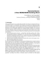
To illustrate the application of these ideas, consider a circular disk D rolling to the left
in a straight line on a surface S as in Figure 5.8.2. Let Q be the center of D, let O be the
contact point (instant center of zero velocity) of D with S, and let P be a point on the
periphery or rim of D. Finally, let D have radius r, angular speed ω, and angular acceler-
ation α, as indicated.
Because Q moves on a straight line, its velocity may be expressed as:
(5.8.26)
Then, by differentiating, the acceleration of Q is:
(5.8.27)
Because O and P are also fixed on D, their velocities and acceleration may be obtained
from the expressions:
(5.8.28)
and
(5.8.29)
By substituting from Eqs. (5.8.26) and (5.8.27), by recognizing that ωω
ωω
and αα
αα
are ωn
z
and
αn
z
, and by carrying out the indicated operations, we obtain:
(5.8.30)
FIGURE 5.8.2
A rolling disk.
D

S
O
Q
P
α
ω
n
n
n
y
x
z
ξ
α
αω
η
ω
αω
ξη
αω
2
2
24
2
2
4
24
2
2
24

1
=
+
()
=
+
()
+=
+
, , and
2
αξξη ωηξη=+
()
=+
()
//
22 2 22
and
vn
Q
x
r=− ω
av n
QQ
x
ddtr==−α
vv n vv n
OQ
y
PQ

y
rr=+×−
()
=+×
()
ωωωω,
aa n n aa n n
OQ
yy
PQ
yy
rr rr=+×−
()
+× ×−
()
[]
=+×
()
+× ×
()
[]
ααωωωωααωωωω,
vnnn
O
xz y
rr=− + × −
()
=ωω 0
0593_C05_fm Page 153 Monday, May 6, 2002 2:15 PM
154 Dynamics of Mechanical Systems

(5.8.31)
(5.8.32)
(5.8.33)
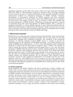
Observe that the velocity of O is zero, as expected, but the acceleration of O is not zero.
To find the point C with zero acceleration, we can use Eqs. (5.8.11) and (5.8.12): specifically,
for a Cartesian (X–Y) axes system with origin at O, we find the coordinates of C to be:
(5.8.34)
and
(5.8.35)
For positive values of ω and α, the position of C is depicted in Figure 5.8.3.
To verify the results, consider calculating the acceleration of C using the expression:
(5.8.36)
where QC is:
(5.8.37)
Using Eq. (5.8.27), a
C
becomes:
(5.8.38)
Finally, we can check the consistency of Eqs. (5.8.18), (5.8.21), and (5.8.22): from Eqs.
(5.8.21) and (5.8.22), ξ and η are:
(5.8.39)
vnnn n
P
xzy x
rrr=− + ×
()
=−ωω ω2
annnnnn n
O
xz y z z y y

rr rr=− + × −
()
+× ×−
()
[]
=αα ω ω ω
2
annnnnn
nn
P
xzy z zy
xy
rr r
rr
=− + ×
()
+× ×
()
[]
=− −
αα ω ω
αω2
2
xx
xy
r
r
CQ
QQ
=+

−
+
=+
−
()
−
()
+
=−
+
ωα
αω
ωαα
αω
αω
αω
2
24
2
24
2
24
0
0
˙˙
˙˙
yy
xy
r
r

r
CQ
QQ
=+
+
+
=+
−
()
+
()
+
=
+
αω
αω
ααω
αω
ω
αω
˙˙
˙˙
2
24
2
24
4
24
0
a a QC QC

CQ
=+× +×
()
ααωω
QC n n=−
+
−−
+












r
r
r
xy
αω
αω
ω
αω
2
24

4
24
an n n
nn
C
xy x
xy
r
r
r
r
r
r
r
=− −
+
+−
+













+
+
+−
+












=
αα
αω
αω
α
ω
αω
ω
αω
αω
ω
ω
αω
2

24
4
24
2
2
24
2
4
24
0
ξ= −
()
−
()
−−
()
−
()
[]
1
∆
xxyy yyxx
PQQP PQQP
˙˙ ˙˙
˙˙ ˙˙
0593_C05_fm Page 154 Monday, May 6, 2002 2:15 PM
Planar Motion of Rigid Bodies — Methods of Analysis 155
and
(5.8.40)
where, from Eq. (5.8.23), ∆ is:

(5.8.41)
From Eqs. (5.8.27) and (5.8.33) and from Figure 5.8.3 we have:
(5.8.42)
Then, ∆ becomes:
(5.8.43)
Hence, ξ and η are:
(5.8.44)
(5.8.45)
These expressions are identical with those of Eq. (5.8.18).
FIGURE 5.8.3
Location of center C of zero acceler-
ation for rolling disk of Figure 5.8.2.
D
O
Q
P
α
ω
n
n
y
x
C
X
r ω
α + ω
Y
r α ω
α + ω
4

4
2
2
2
4
η= −
()
−
()
−−
()
−
()
[]
1
∆
yyyy xxxx
PQPQ PQQP
˙˙ ˙˙
˙˙ ˙˙
∆=− −
()
+−
()







˙˙ ˙˙
˙˙ ˙˙
yy xx
PQ QP
22
xyr
xyr
xr yr
xr y
PP
QQ
PP
QQ
==
==
=− =−
=− =
02
0
2
0
2
,
,
˙˙
,
˙˙
˙˙
,
˙˙

αω
α
∆=− − −
()
+− +
()






=− +
()
rrrrωααωα
2
2
2
24 2
02
ξ
ωα
αα
α
αω
=
−
+
()
−−

()
−+
()
[]
=
+
1
02 2
24 2
24
r
rr r r
η
ωα
ω
ω
αω
=
−
+
()
−
()
−−
()
−
[]
=
+
1

200
24 2
2
2
24
r
rr r
0593_C05_fm Page 155 Monday, May 6, 2002 2:15 PM
156 Dynamics of Mechanical Systems
Problems
Section 5.2 Coordinates, Constraints, Degrees of Freedom
P5.2.1: Consider a pair of eyeglasses to be composed of a frame containing the lenses and
two rods hinged to the frame for fitting over the ears. How many degrees of freedom do
the eyeglasses have?
P5.2.2: Let a simple model of the human arm consist of three bodies representing the
upper arm, the lower arm, and the hands. Let the upper arm have a spherical (ball-and-
socket) connection with the chest, let the elbow be represented as a pin (or hinge), and
let the hand movement be governed by a twist of the lower arm and vertical and horizontal
rotations. How many degrees of freedom does the model have?
P5.2.3: How many degrees of freedom does a vice, as commonly found in a workshop,
have? (Include the axial rotation of the adjustment handle about its long axis and the
potential rotation of the vice itself about a vertical axis.)
P5.2.4: See Figure P5.2.4. A wheel W, having planar motion, rolls without slipping in a
straight line. Let C be the contact point between W and the rolling surface S. How many
degrees of freedom does W have? What are the constraint equations?
P5.2.5: See Problem P5.2.4. Suppose W is allowed to slip along S. How many degrees of
freedom does W then have?
P5.2.6: How many degrees of freedom are there in a child’s tricycle whose wheels roll
without slipping on a flat horizontal surface? (Neglect the rotation of the pedals about
their individual axes.)

Section 5.3 Planar Motion of a Rigid Body
P5.3.1: Classify the movement of the following bodies as being (1) translation, (2) rotation,
and/or (3) general plane motion.
a. Eraser on a chalk board
b. Table-saw blade
c. Radial-arm-saw blade
d. Bicycle wheel of a bicycle moving in a straight line
e. Seat of a bicycle moving in a straight line
f. Foot pedal of a bicyclist moving in a straight line
FIGURE P5.2.4
A wheel rolling in a straight line.
C
S
W
0593_C05_fm Page 156 Monday, May 6, 2002 2:15 PM