Adaptive Control System Part 8 pdf
Bạn đang xem bản rút gọn của tài liệu. Xem và tải ngay bản đầy đủ của tài liệu tại đây (239.06 KB, 25 trang )
considerations, a new class of uncertain nonlinear systems with unmodelled
dynamics has been considered in the second part of this chapter. A novel
recursive robust adaptive control method by means of backstepping and small
gain techniques was proposed to generate a new class of adaptive nonlinear
controllers with robustness to nonlinear unmodelled dynamics.
It should be mentioned that passivity and small gain ideas are naturally
complementary in stability theory [5]. However, this idea has not been used in
nonlinear control design. We hope that the passivation and small gain
frameworks presented in this chapter show a possible avenue to approach
this goal.
Acknowledgements. This work was supported by the Australian Research
Council Large Grant Ref. No. A49530078. We are very grateful to Laurent
Praly for helpful discussions that led to the development of the result in
subsection 6.4.4.2.
References
[1] Byrnes, C. I. and Isidori, A. (1991) `Asymptotic Stabilization of Minimum-Phase
Nonlinear Systems', IEEE Trans. Automat. Control, 36, 1122±1137.
[2] Byrnes, C. I., Isidori, A. and Willems, J.C. (1991) `Passivity, Feedback
Equivalence, and the Global Stabilization of Minimum Phase Nonlinear
Systems', IEEE Trans. Automat. Control, 36, 1228±1240.
[3] Corless, M. J. and Leitmann, G. (1981) `Continuous State Feedback Guaranteeing
Uniform Ultimate Boundedness for Uncertain Dynamic Systems', IEEE Trans.
Automat. Control, 26, 1139±1144.
[4] Coron, J. -M., Praly, L. and Teel, A. (1995) `Feedback Stabilization of Nonlinear
Systems: Sucient Conditions and Lyapunov and Input-Output Techniques'. In:
Trends in Control (A. Isidori, ed.) 293±348, Springer.
[5] Desoer, C. A. and Vidyasagar, M. (1975) `Feedback Systems: Input-Output
Properties'. New York: Academic Press.
[6] Fradkov, A. L., Hill, D. J., Jiang, Z. P. and Seron, M. M. (1995) `Feedback
Passi®cation of Interconnected Systems', Prep. IFAC NOLCOS'95, 660±665,
Tahoe City, California.
[7] Hahn, W. (1967) Stability of Motion. Springer-Verlag.
[8] Hardy, G., Littlewood, J. E. and Polya, G. (1989) Inequalities. 2nd Edn,
Cambridge University Press.
[9] Hill, D. J. (1991) `A Generalization of the Small-gain Theorem for Nonlinear
Feedback Systems', Automatica, 27, 1047±1050.
[10] Hill, D. J. and Moylan, P. (1976) `The Stability of Nonlinear Dissipative Systems',
IEEE Trans. Automat. Contr., 21, 708±711.
[11] Hill, D. J. and Moylan, P. (1977) `Stability Results for Nonlinear Feedback
Systems', Automatica, 13, 377±382.
[12] Hill, D. J. and Moylan, P. (1980) `Dissipative Dynamical Systems: Basic Input±
Output and State Properties', J. of The Franklin Institute, 309, 327±357.
156 Adaptive nonlinear control: passivation and small gain techniques
[13] Ioannou, P. A. and Sun, J. (1996) Robust Adaptive Control. Prentice-Hall, Upper
Saddle River, NJ.
[14] Jiang, Z. P. and Hill, D. J. (1997) `Robust Adaptive Nonlinear Regulation with
Dynamic Uncertainties', Proc. 36th IEEE Conf. Dec. Control, San Diego, USA.
[15] Jiang, Z. P. and Hill, D. J. (1998) `Passivity and Disturbance Attenuation via
Output Feedback for Uncertain Nonlinear Systems', IEEE Trans. Automat.
Control, 43, 992±997.
[16] Jiang, Z. P. and Mareels, I. (1997) `A Small Gain Control Method for Nonlinear
Cascaded Systems with Dynamic Uncertainties', IEEE Trans. Automat. Contr., 42,
292±308.
[17] Jiang, Z. P. and Praly, L. (1996) `A Self-tuning Robust Nonlinear Controller',
Proc. 13th IFAC World Congress, Vol. K, 73±78, San Francisco.
[18] Jiang, Z. P. and Praly, L. (1998) `Design of Robust Adaptive Controllers for
Nonlinear Systems with Dynamic Uncertainties', Automatica, Vol. 34, No. 7,
825±840.
[19] Jiang, Z. P., Hill, D. J. and Fradkov, A. L. (1996) `A Passi®cation Approach to
Adaptive Nonlinear Stabilization', Systems & Control Letters, 28, 73±84.
[20] Jiang, Z. P., Mareels, I. and Wang, Y. (1996) `A Lyapunov Formulation of the
Nonlinear Small-gain Theorem for Interconnected ISS Systems', Automatica, 32,
1211±1215.
[21] Jiang, Z. P., Teel, A. and Praly, L. (1994) `Small-gain Theorem for ISS Systems and
Applications', Mathematics of Control, Signals and Systems, 7, 95±120.
[22] Kanellakopoulos, I., Kokotovic
Â
, P. V. and Marino, R. (1991) `An Extended Direct
Scheme for Robust Adaptive Nonlinear Control', Automatica, 27, 247±255.
[23] Kanellakopoulos, I., Kokotovic
Â
, P. V. and Morse, A. S. (1992) `A Toolkit for
Nonlinear Feedback Design', Systems & Control Letters, 18, 83±92.
[24] Khalil, H. K. (1996) Nonlinear Systems. 2nd Edn, Prentice-Hall, Upper Saddle
River, NJ.
[25] Kokotovic
Â
, P. V. and Sussmann, H. J. (1989) `A Positive Real Condition for
Global Stabilization of Nonlinear Systems', Systems & Control Letters, 13, 125±
133.
[26] Krstic
Â
, M., Kanellakopoulos, I., and Kokotovic
Â
, P. V. (1995) Nonlinear and
Adaptive Control Design. New York: John Wiley & Sons.
[27] Kurzweil, J. (1956) `On the Inversion of Lyapunov's Second Theorem on Stability
of Motion', American Mathematical Society Translations, Series 2, 24, 19±77.
[28] Lin, Y. (1996) `Input-to-state Stability with Respect to Noncompact Sets, Proc.
13th IFAC World Congress, Vol. E, 73±78, San Francisco.
[29] Lozano, R., Brogliato, B. and Landau, I. (1992) `Passivity and Global Stabilization
of Cascaded Nonlinear Systems', IEEE Trans. Autom. Contr., 37
, 1386±1388.
[30] Mareels, I. and Hill, D. J. (1992) `Monotone Stability of Nonlinear Feedback
Systems', J. Math. Systems Estimation Control, 2, 275±291.
[31] Marino, R. and Tomei, P. (1993) `Robust Stabilization of Feedback Linearizable
Time-varying Uncertain Nonlinear Systems', Automatica, 29, 181±189.
[32] Marino, R. and Tomei, P. (1995) Nonlinear Control Design: Geometric, Adaptive
and Robust. Prentice-Hall, Europe.
Adaptive Control Systems 157
[33] Moylan, P. and Hill, D. (1978) `Stability Criteria for Large-scale Systems', IEEE
Trans. Autom. Control, 23, 143±149.
[34] Ortega, R. (1991) `Passivity Properties for the Stabilization of Cascaded Nonlinear
Systems', Automatica, 27, 423±424.
[35] Polycarpou, M. M. and Ioannou, P. A. (1995) `A Robust Adaptive Nonlinear
Control Design. Automatica, 32, 423±427.
[36] Praly, L. and Jiang, Z P. (1993) `Stabilization by Output Feedback for Systems
with ISS Inverse Dynamics', Systems & Control Letters, 21, 19±33.
[37] Praly, L., Bastin, G., Pomet, J B. and Jiang, Z. P. (1991) `Adaptive Stabilization of
Nonlinear Systems, In Foundations of Adaptive Control (P.V. Kokotovic
Â
, ed.), 347±
433, Springer-Verlag.
[38] Rodriguez, A. and Ortega, R. (1990) `Adaptive Stabilization of Nonlinear Systems:
the Non-feedback Linearizable Case', in Prep. of the 11th IFAC World Congress,
121±124.
[39] Safanov, M. G. (1980) Stability and Robustness of Multivariable Feedback Systems.
Cambridge, MA: The MIT Press.
[40] Sepulchre, R., Jankovic
Â
, M. and Kokotovic
Â
, P. V. (1996) `Constructive Nonlinear
Control. Springer-Verlag.
[41] Seron, M. M., Hill, D. J. and Fradkov, A. L. (1995) `Adaptive Passi®cation of
Nonlinear Systems', Automatica, 31, 1053±1060.
[42] Sontag, E. D. (1989) `Smooth Stabilization Implies Coprime Factorization', IEEE
Trans. Automat. Contr., 34, 435±443.
[43] Sontag, E. D. (1989) `Remarks on Stabilization and Input-to-state Stability', Proc.
28th Conf. Dec. Contr., 1376±1378, Tampa.
[44] Sontag, E. D. (1990) `Further Facts about Input-to-state Stabilization', IEEE
Trans. Automat. Contr., 35, 473±476.
[45] Sontag, E. D. (1995) `On the Input-to-State Stability Property', European Journal
of Control, 1, 24±36.
[46] Sontag, E. D. and Wang, Y. (1995) `On Characterizations of the Input-to-state
Stability Property', Systems & Control Letters, 24, 351±359.
[47] Sontag, E. D. and Wang, Y. (1995) `On Characterizations of Set Input-to-state
Stability', in Prep. IFAC Nonlinear Control Systems Design Symposium
(NOLCOS'95), 226±231, Tahoe City, CA.
[48] Taylor, D. G., Kokotovic
Â
, P. V., Marino, R. and Kanellokopoulos, I. (1989)
`Adaptive Regulation of Nonlinear Systems with Unmodeled Dynamics', IEEE
Trans. Automat. Contr., 34, 405±412.
[49] Teel, A. and Praly, L. (1995) `Tools for Semiglobal Stabilization by Partial-state
and Output Feedback', SIAM J. Control Optimiz., 33, 1443±1488.
[50] Willems, J. C. (1972) `Dissipative Dynamical Systems, Part I: General Theory; Part
II: Linear Systems with Quadratic Supply Rates', Archive for Rational Mechanics
and Analysis, 45, 321±393.
[51] Yao, B. and Tomizuka, M. (1995) `Robust Adaptive Nonlinear Control with
Guaranteed Transient Performance', Proceedings of the American Control
Conference, Washington, 2500±2504.
158 Adaptive nonlinear control: passivation and small gain techniques
7
Active identi®cation for
control of discrete-time
uncertain nonlinear
systems
J. Zhao and I. Kanellakopoulos
Abstract
The problem of controlling nonlinear systems with unknown parameters has
received a great deal of attention in the continuous-time case. In contrast, its
discrete-time counterpart remains largely unexplored, primarily due to the
diculties associated with utilizing Lyapunov design techniques in a discrete-
time framework. Existing results impose restrictive growth conditions on the
nonlinearities to yield global stability.
In this chaper we propose a novel approach which removes this obstacle and
yields global stability and tracking for systems that can be transformed into an
output-feedback, strict-feedback, or partial-feedback canonical form. The
main novelties of our design are: (i) the temporal and algorithmic separation
of the parameter estimation task from the control task, and (ii) the develop-
ment of an active identi®cation procedure, which uses the control input to
actively drive the system state to points in the state space that allow the
orthogonalized projection estimator to acquire all the necessary information
about the unknown parameters. We prove that our algorithm guarantees
complete (for control purposes) identi®cation in a ®nite time interval, whose
maximum length we compute.
Thus, the traditional structure of concurrent on-line estimation and control
is replaced by a two-phase control strategy: ®rst use active identi®cation, and
then utilize the acquired parameter information to implement any control
strategy as if the parameters were known.
7.1 Introduction
In recent years, a great deal of progress has been made in the area of adaptive
control of continuous-time nonlinear systems [1], [2]. In contrast, adaptive
control of discrete-time nonlinear systems remains a largely unsolved problem.
The few existing results [3, 4, 5, 6] can only guarantee global stability under
restrictive growth conditions on the nonlinearities, because they use techniques
from the literature on adaptive control of linear systems [7, 8]. Indeed, it has
recently been shown that any discrete-time adaptive nonlinear controller using
a least-squares estimator cannot provide global stability in either the determi-
nistic [9] or the stochastic [10] setting. The only available result which
guarantees global stability without imposing any such growth restrictions is
found in [11], but it only deals with a scalar nonlinear system which contains a
single unknown parameter.
The backstepping methodology [1], which provided a crucial ingredient for
the development of solutions to many continuous-time adaptive nonlinear
problems, has a very simple discrete-time counterpart: one simply `looks ahead'
and chooses the control law to force the states to acquire their desired values
after a ®nite number of time steps. One can debate the merits of such a
deadbeat control strategy [12], especially for nonlinear systems [13], but it seems
that in order to guarantee global stability in the presence of arbitrary non-
linearities, any controller will have to have some form of prediction capability.
In the presence of unknown parameters, however, it is impossible to calculate
these `look-ahead' values of the states. Furthermore, since these calculations
involve the unknown parameters as arguments of arbitrary nonlinear func-
tions, no known parameter estimation method is applicable, since all of them
require a linear parametrization to guarantee global results. This is the biggest
obstacle to providing global solutions for any of the more general discrete-time
nonlinear problems.
In this chapter we introduce a completely dierent approach to this problem,
which allows us to obtain globally stabilizing controllers for several classes of
discrete-time nonlinear systems with unknown parameters, without imposing
any growth conditions on the nonlinearities. The major assumptions are that
the unknown parameters appear linearly in the system equations, and that the
system at hand can be transformed, via a global parameter-independent
dieomorphism, into one of the canonical forms that have been previously
considered in the continuous-time adaptive nonlinear control literature [1].
Another major assumption is that our system is free of noise; this allows us
to replace the usual least-squares parameter estimator with an orthogonalized
projection scheme, which is known to converge in ®nite time, provided the
actual values of the regressor vector form a basis for the regressor subspace.
The main diculty with this type of estimator is that in general there is no way
to guarantee that this basis will be formed in ®nite time. The ®rst steps towards
160 Active identi®cation for control of discrete-time uncertain nonlinear systems
removing this obstacle were taken in preliminary versions of this work [14, 15].
In those papers we developed procedures for selecting the value of the control
input during the initial identi®cation period in a way that drives the system
state towards points in the state space that generate a basis for this subspace in
a speci®ed number of time steps. In this chapter we integrate those procedures
with the orthogonalized projection estimator to construct a true active
identi®cation scheme, which produces a parameter estimate in a familiar
recursive (and thus computationally ecient) manner, and at each time instant
uses the current estimate to compute the appropriate control input. As a result,
we guarantee that all the parameter information necessary for control purposes
will be available after at most 2nr steps for output-feedback systems and
n 1r steps for strict-feedback systems, where n is the dimension of the
system and r is the dimension of the regressor subspace. If the number of
unknown parameters p is equal to r, as it would be in any well-posed
identi®cation problem, this implies that at the end of the active identi®cation
phase the parameters are completely known. If, on the other hand, p > r, then
we only identify the projection of the parameter vector that is relevant to the
system at hand, and that is all that is necessary to implement any control
algorithm. In essence, our active identi®cation scheme guarantees that all the
conditions for persistent excitation will be satis®ed in a ®nite time interval: in
the noise-free case and for the systems we are considering, all the parameter
information that could be acquired by any identi®cation procedure in any
amount of time, will in fact be acquired by our scheme in an interval which is
made as short as possible, and whose upper bound is computed a priori. The
fact that our scheme attempts to minimize the length of this interval is
important for transient performance considerations, since this will prevent
the state from becoming too large during the identi®cation phase.
Once this active identi®cation phase is over, the acquired parameter
information can be used to implement any control algorithm as if the
parameters were completely known. As an illustration, in this chapter we use
a straightforward deadbeat strategy. The fact that discrete-time systems (even
nonlinear ones) cannot exhibit the ®nite escape time phenomenon, makes it
possible to delay the control action until after the identi®cation phase and still
be able to guarantee global stability.
7.2 Problem formulation
The systems we consider in this section comprise all systems that can be
transformed via a global dieomorphism to the so-called parametric-output-
Adaptive Control Systems 161
feedback form:
x
1
t 1x
2
t
1
x
1
t
F
F
F
x
nÀ1
t 1x
n
t
nÀ1
x
1
t
x
n
t 1ut
n
x
1
t
ytx
1
t
7:1
where P R
p
is the vector of unknown constant parameters and
i
, i 1; FFF; n
are known nonlinear functions. The name `parametric-output-feedback form'
denotes the fact that the nonlinearities
i
that are multiplied by unknown
parameters depend only on the output y x
1
, which is the only measured
variable; the states x
2
; FFF; x
n
are not measured. It is important to note that the
functions
i
are not restricted by any type of growth conditions; in fact, they
are not even assumed to be smooth or continuous. The only requirement is that
they take on ®nite values whenever their argument x
1
is ®nite; this excludes
nonlinearities like
1
x
1
À 1
, for example, but it is necessary since we want to
obtain global results. This requirement also guarantees that the solutions of
(7.1) (with any control law that remains ®nite for ®nite values of the state
variables) exist on the in®nite time interval, i.e. there is no ®nite escape time.
Furthermore, no restrictions are placed on the values of the unknown constant
parameter vector or on the initial conditions. However, the form (7.1) already
contains several structural restrictions: the unknown parameters appear
linearly, the nonlinearities are not allowed to depend on the unmeasured
states, and the system is completely noise free: there is no process noise, no
sensor noise, and no actuator noise.
Our control objective consists of the global stabilization of (7.1) and the
global tracking of a known reference signal y
d
t by the output x
1
t.
For notational simplicity, we will denote
i;t
i
x
1
t for i 1; FFF n.
7.2.1 A second-order example
To illustrate the diculties present in this problem, let us consider the case
when the system (7.1) is of second order, i.e.
x
1
t 1x
2
t
1;t
x
2
t 1ut
2;t
ytx
1
t
7:2
Even if were known, the control ut would only be able to aect the output
162 Active identi®cation for control of discrete-time uncertain nonlinear systems
x
1
at time t 2. In other words, given any initial conditions x
1
0 and x
2
0,we
have no way of in¯uencing x
1
1 through u0. The best we can do is to drive
x
1
2 to zero and keep it there. The control would simply be a deadbeat
controller, which utilizes our ability to express future values of x
1
as functions
of current and past values of x
1
and u:
x
1
t 2x
2
t 1
1;t1
ut
2;t
1;t1
ÂÃ
ut
2;t
1
x
2
t
1;t
ÂÃ
ut
2;t
1
ut À1
2;tÀ1
1;t
ÂÃ
7:3
Thus, the choice of control
uty
d
t 2À
2;t
1;t1
ÂÃ
y
d
t 2À
2;t
1
ut À1
2;tÀ1
1;t
ÀÁÂÃ
; t ! 1 7:4
would yield x
1
ty
d
t for all t ! 3 and would achieve the objective of global
stabilization.
We emphasize that here we use a deadbeat control law only because it makes
the presentation simpler. All the arguments made here are equally applicable to
any other discrete-time control strategy, as is the parameter information
supplied by our active identi®cation procedure. We hasten to add, however,
that, from a strictly technical point of view, deadbeat control is perfectly
acceptable in this case, for the following two reasons:
(1) The well-known problems of poor inter-sample behaviour resulting from
applying deadbeat control to sampled-data systems do not arise here, since
we are dealing with a purely discrete-time problem.
(2) Deadbeat control can result to instability when applied to general
polynomial nonlinear systems. As an example, consider the system
x
1
t 1x
2
tx
1
tx
2
2
t
x
2
t 1ut
ytx
1
t
7:5
If we implement a deadbeat control strategy to track the reference signal
y
d
t2
Àt
, one of the two possible closed-form solutions yields
x
2
tÀ2
t
À
1 2
2t
p
7:6
which is clearly unbounded. The computational procedures presented in
[13] provide ways of avoiding such problems. However, in the case of
systems of the form (7.1) and of all the other forms we deal with in this
Adaptive Control Systems 163
chapter, such issues do not even arise, owing to the special structure of our
systems which guarantees that boundedness of x
1
; FFF; x
i
automatically
ensures boundedness of x
i1
, since x
i1
tx
i
t 1À
i
x
1
t.
Of course, when is unknown, the controller (7.4) cannot be implemented.
Furthermore, it is clear that any attempt to replace the unknown with an
estimate
would be sti¯ed by the fact that appears inside the nonlinear
function
1
. Available estimation methods cannot provide global results for
such a nonlinearly parametrized problem, except for the case where
1
is
restricted by linear growth conditions.
7.2.2 Avoiding the nonlinear parametrization
Our approach to this problem does not solve the nonlinear parametrization
problem; instead, it bypasses it altogether. Returning to the control expression
(7.4), we see that its implementation relies on the ability to compute the term
2;t
1;t1
7:7
Since this computation must happen at time t, the argument x
1
t 1 is not yet
available, so it must be `pre-computed' from the expression
x
1
t 1x
2
t
1;t
ut À 1
2;tÀ1
1;t
7:8
Careful examination of the expressions (7.4)±(7.8) reveals that our controller
would be implementable if we had the ability to calculate the projection of the
unknown parameter vector along known vectors of the form
2
x
1
~
x7:9
since then we would be able at time t to compute the terms
2;tÀ1
1;t
7:10
2;t
1;t1
7:11
and from them the control (7.4).
Hence, our main task is to compute the projection of along vectors of the
form (7.9). To achieve this, we proceed as follows:
Regressor subspace: First, we de®ne the subspace spanned by all vectors of
the form (7.9):
S
0
D
f
1
x
2
~
x; Vx P R; V
~
x P Rg7:12
Note that the known nonlinear functions
1
and
2
need to be evaluated
independently over all possible values of their arguments. This is necessary
because we are not imposing any smoothness or continuity assumptions on
164 Active identi®cation for control of discrete-time uncertain nonlinear systems
these functions. However, for any reasonable nonlinearities, determining this
subspace will be a fairly straightforward task which of course can be performed
o-line. The dimension of S
0
, denoted by r
0
, will always be less than or equal
to the number of unknown parameters p: r
0
p. In fact, in any reasonably
posed problem we will have r
0
p, since r
0
< p means that we are considering
more parameters than are actually entering the system equations; in that case,
complete parameter identi®cation cannot be achieved with any method or
input, since the regressor vector cannot acquire the values necessary to identify
some of the parameters. Hence, if r
0
< p, then the number of unknown
parameters can be reduced to r
0
without any loss of information or generality.
Projection measurements Clearly, in order to be able to implement the control
(7.4), all we need to know about is its projection on the subspace S
0
. But how
do we acquire this projection? From (7.3) we see that at time t, using the
measurements x
1
t; x
1
t À1; x
1
t À2 and the known value of the control
ut À2, we can compute the following projection:
2
x
1
t À2
1
x
1
t À1x
1
tÀut À27:13
Hence, if the values of x
1
are such that the corresponding values of the vector
2
x
1
t À2
1
x
1
t À1 eventually form a basis for the subspace S
0
,we
will obtain all the necessary information about . But how do we guarantee
that this identi®cation phase will be of ®nite duration?
Active identi®cation Instead of allowing the system state to drift on its own,
we use the control input u to drive the output x
1
to values which result in
linearly independent vectors
2;tÀ2
1;tÀ1
and form a basis for S
0
in at most
2nr
0
steps (where n is the dimension of the system state and r
0
the dimension of
the nonlinearity subspace). But how can we determine the values of u that will
result in such basis vectors in the presence of unknown parameters? This
seemingly hopeless dilemma can be resolved by the following observation,
which will be clari®ed further later on:
The expression (7.4) is not computable if and only if at least one of the
vectors
2;tÀ1
1;t
and
2;t
1;t1
is independent of the past values
2;jÀ1
1;j
; j t À1. Thus, inability to compute (7.4) from already meas-
ured projections is equivalent to the knowledge that new independent
directions are being generated by the system.
In other words, whenever our identi®cation process gets `stuck', that is, the
system does not generate new directions over the next few steps, then the
projection information we have already acquired is enough for us to compute a
value of control which will get the system `unstuck' and will generate a new
direction after at most 2n (in this case 4) steps: this is the time it takes to change
the arguments of both
1
and
2
and measure the resulting projection.
Adaptive Control Systems 165
Orthogonalized projection estimation All the projection information of is
automatically incorporated into the parameter estimate
produced by an
orthogonalized projection algorithm. This means that after the active identi-
®cation phase is complete, all the terms appearing in (7.10) and (7.11) can be
computed simply by replacing by its estimate
. This allows us to proceed
with the implementation of the controller (7.4) or any other control strategy as
if the parameters were known.
Clearly, this two-stage process depends critically on the fact that, contrary to
their continuous-time counterparts, discrete-time nonlinear systems cannot
exhibit ®nite escape times, as long as their nonlinearities take on ®nite values
whenever their arguments are ®nite. This property allows us to postpone
closing the loop with a controller until after the ®nite-duration identi®cation
phase has been completed.
7.3 Active identi®cation
Let us now elaborate further on the above outlined approach by presenting in
detail its two most challenging ingredients, namely the pre-computation
scheme and the input selection for active identi®cation. To do this, we return
to the general output-feedback form (7.1) and rewrite it in the following scalar
form:
x
1
t nx
2
t n À1
1
x
1
t n À1
x
3
t n À2
2
x
1
t n À2
1
x
1
t n À1
F
F
F
ut
n
k1
k
x
1
t n Àk 7:14
Hence, the following choice of a deadbeat control law:
uty
d
t nÀ
n
k1
k;tnÀk
7:15
will globally stabilize the system (7.1) and yield x
1
ty
d
t; t ! n.
Clearly, the implementation of the control law (7.15) requires us to calculate
(at time t) the projection of the unknown along the vector
n
k1
k;tnÀk
. This
means that we need to compute the value of
n
k1
k;tnÀk
at time t. Rewriting
n
k1
k;tnÀk
as
n
k1
k;tnÀk
n
k1
k
x
1
t n Àk 7:16
we can therefore infer that it is necessary for us to be able to calculate the value
166 Active identi®cation for control of discrete-time uncertain nonlinear systems
of the states x
1
t 1; FFF; x
1
t n À1 at time t. To see how to calculate these
states, let us return to equation (7.14) and express x
1
t 1; FFF; x
1
t n À1
as
x
1
t iut Àn i
n
k1
k
x
1
t i À k; i 1; FFF; n À 1 7:17
Clearly, equation (7.17) shows that the value of x
1
t 1 depends on the values
of both
n
k1
k;t1Àk
and ut Àn 1. Since the values of ut Àn 1 and
the vector
n
k1
k;t1Àk
are known at time t, the key to successfully calculating
(at time t) the value of x
1
t 1 depends on whether we are able to compute
the projection of the unknown along the vector
n
k1
k;t1Àk
at time t.
Next, let us examine what we need to calculate the value of x
1
t 2 at time
t. From (7.17), the value of x
1
t 2 is equal to the sum of ut À n 2 and
n
k1
k;t2Àk
. Clearly, if we are able to calculate the values of both
ut Àn 2 and
n
k1
k;t2Àk
at time t, then the value of x
2
t 2 can be
acquired (at time t). The value of ut Àn 2 is known at time t, while from
the expression
n
k1
k;t2Àk
1;t1
n
k2
k;t2Àk
1
x
1
t 1
nÀ1
k1
k1
x
1
t 1 Àk
7:18
we see that the value of
n
k1
k;t2Àk
depends on x
1
t 1. This means that
pre-computing the value of x
2
t 2 requires the values of both x
1
t 1 and
n
k1
k;t2Àk
. In view of the discussion of the previous paragraph, the
calculation of x
1
t 1 at time t requires us to compute (at time t) the value of
n
k1
k;t1Àk
. Thus, in summary, the calculation of x
1
t 2 requires us to
pre-compute (at time t) the values of
n
k1
k;t1Àk
n
k1
k;t2Àk
45
7:19
Generalizing the argument of the previous two paragraphs, we can conclude
that the pre-computation of the value of x
1
t l (1 l n À 1) requires
knowledge (at time t) of the vector
n
k1
k;t1Àk
F
F
F
n
k1
k;tlÀk
P
T
T
R
Q
U
U
S
7:20
Adaptive Control Systems 167
Hence, the knowledge (at time t) of the above vector with l n À 1
n
k1
k;t1Àk
F
F
F
n
k1
k;tnÀ1Àk
P
T
T
R
Q
U
U
S
7:21
enables us to determine the values of the states x
1
t 1; FFF; x
1
t n À1 at
time t. However, the implementation of the control law (7.15) requires the
value of
n
k1
k;tnÀk
also. This leads ®nally to the conclusion that, in order
to use the control law (7.15), we need to pre-compute (at time t) the vector
n
k1
k;t1Àk
F
F
F
n
k1
k;tnÀk
P
T
T
R
Q
U
U
S
7:22
The procedure for acquiring (7.22) at time t (t ! n) is given in the next two
sections, whose contents can be brie¯y summarized as follows: ®rst, the section
on pre-computation explains how to pre-compute the vector (7.22) after the
identi®cation phase is complete, that is, for any time t such that S
0
tÀ1
S
0
,
where S
0
tÀ1
denotes the subspace that has been identi®ed at time t (with t > n):
S
0
tÀ1
D
n
k1
k;iÀk
; i n; FFF; t
@A
7:23
while S
0
denotes the subspace formed by all possible values of the regressor
vector:
S
0
D
n
i1
i
z
i
; Vz
1
; FFF; z
n
PR
n
@A
; r
0
D
dim S
0
7:24
Then, the section on input selection for identi®cation shows how to guarantee
that the identi®cation phase will be completed in ®nite time, that is, how to
ensure the existence of a ®nite time t
f
at which S
0
t
f
À1
S
0
. In addition, we will
show that t
f
2nr
0
.
The reason for this seemingly inverted presentation, where we ®rst show
what to do with the results of the active identi®cation and then discuss how to
obtain these results, is that it makes the procedure easier to understand.
7.3.1 Pre-computation of projections
The pre-computation of (7.22) is implemented through an orthogonalized
projection estimator. Therefore, we ®rst review brie¯y the standard version
of this estimation scheme; for more details, the reader is referred to Section 3.3
of [7].
168 Active identi®cation for control of discrete-time uncertain nonlinear systems
Orthogonalized projection algorithm Consider the problem of estimating an
unknown parameter vector from a simple model of the following form:
ytt À1
7:25
where yt denotes the (scalar) system output at time t, and t À1 denotes a
vector that is a linear or nonlinear function of past measurements
t À 1fyt À1; yt À2; FFFg
t À1fut À 1; ut À2; FFFg
7:26
The orthogonalized projection algorithm for (7.25) starts with an initial
estimate
0
and the p Âp identity matrix P
À1
, and then updates the estimate
and the covariance matrix P for t ! 1 through the recursive expressions:
t
tÀ1
P
tÀ2
tÀ1
tÀ1
P
tÀ2
tÀ1
ytÀ
tÀ1
tÀ1
if
tÀ1
P
tÀ2
tÀ1
T 0
tÀ1
if
tÀ1
P
tÀ2
tÀ1
0
V
b
b
`
b
b
X
7:27
P
tÀ1
P
tÀ2
À
P
tÀ2
tÀ1
tÀ1
P
tÀ2
tÀ1
P
tÀ2
tÀ1
if
tÀ1
P
tÀ2
tÀ1
T 0
P
tÀ2
if
tÀ1
P
tÀ2
tÀ1
0
V
b
b
`
b
b
X
7:28
This algorithm has the following useful properties, which are given here
without proof:
(i) P
tÀ1
t is a linear combination of the vectors 1; FFF;t.
(ii) xP
t
f1; FFF;tg. In other words, P
t
x 0 if and only if x is a
linear combination of the vectors 1; FFF;t.
(iii) P
tÀ1
tcf1; FFF;t À 1g.
(iv)
~
tcf1; FFF;t À 1g, where
~
t
t
À is the parameter estimation
error.
It is worth noting that the orthogonalized projection algorithm produces an
estimate
t
that renders
J
t
t
k1
ykÀ
k À1
2
0 7:29
and thus minimizes this cost function. This implies that orthogonalized
projection is actually an implementable form of the batch least-squares
algorithm, which minimizes the same cost function (7.29). However, the
batch least-squares algorithm, that is, the least-squares algorithm with in®nite
initial covariance (P
À1
À1
0), relies on the necessary conditions for optimality,
Adaptive Control Systems 169
namely
@J
t
@
0 A
t
k1
k À1k À 1
t
k1
ykk À17:30
which cannot be solved to produce a computable parameter estimate before
enough linearly independent measurements have been collected to make the
matrix
t
k1
k À1k À 1
invertible. In contrast, the orthogonalized
projection algorithm produces an estimate which, at each time t, incorporates
all the information about the unknown parameters that has been acquired up
to that time.
Now we are ready to describe how to apply the orthogonalized projection
algorithm (7.27)±(7.28) to our output-feedback system (7.1).
Orthogonalized projection for output-feedback systems At each time t, we can
only measure the output x
1
t. Utilizing this measurement and (7.14), we can
compute the projection of the unknown vector along the known vector
n
k1
k;tÀk
, that is,
"
x
t
n
k1
k
x
1
t Àk
tÀ1
7:31
where
tÀ1
D
n
k1
k;tÀk
and
"
x
t
D
x
1
tÀut Àn for any t with t ! n.
Since equation (7.31) is in the same form as (7.25), we can use the expressions
(7.27)±(7.28) to recursively construct the estimate
t
and the covariance matrix
P
t
(with t ! n 1 in order for (7.31) to be valid), starting from initial estimates
n
and P
nÀ1
I:
1
t
tÀ1
P
tÀ2
tÀ1
tÀ1
P
tÀ2
tÀ1
"
x
t
À
tÀ1
tÀ1
if
tÀ1
P
tÀ2
tÀ1
T 0
tÀ1
if
tÀ1
P
tÀ2
tÀ1
0
V
b
`
b
X
7:32
P
tÀ1
P
tÀ2
À
P
tÀ2
tÀ1
tÀ1
P
tÀ2
tÀ1
P
tÀ2
tÀ1
if
tÀ1
P
tÀ2
tÀ1
T 0
P
tÀ2
if
tÀ1
P
tÀ2
tÀ1
0
V
b
`
b
X
7:33
Lemma 3.1 When the estimation algorithm (7.32)±(7.33) is applied to the
system (7.31), the following properties are true for t ! n:
t
P
tÀ1
t
0 D
t
P S
0
tÀ1
7:34
t
P S
0
tÀ1
A
t1
t
; P
t
P
tÀ1
7:35
170 Active identi®cation for control of discrete-time uncertain nonlinear systems
1
This notation is used in place of the traditional
0
and P
À1
to emphasize the fact
that for the ®rst n time steps we cannot produce any parameter estimates.
v P S
0
tÀ1
A
t
v
tl
v
v; l 0; 1; 2; FFF 7:36
The proof of this lemma is given in the appendix. The properties (7.34)±
(7.36) are crucial to our further development, so let us understand what they
mean. Properties (7.34) and (7.35) state that whenever the regressor vector
t
is
linearly dependent on the past regressor vectors, then our estimator does not
change the value of the parameter estimate and the covariance matrix; this is
due to the fact that the new measurement provides no new projection
information. Property (7.35) states that the estimate
t
produced at time t is
exactly equal to the true parameter vector , when both are projected onto the
subspace spanned by the regressor vectors used to generate this estimate,
namely the subspace S
0
tÀ1
f
0
; FFF;
tÀ1
g. This property is one of the
cornerstones on which we develop our pre-computing methodology in the
following sections, because it implies that at time t we know the projection of
the true parameter vector along the subspace S
0
tÀ1
.
Pre-computation procedure In order to better explain the pre-computation
part of our algorithm, we postulate that there exists a ®nite time instant t
f
! n
at which the regressor vectors that have been measured span the entire
subspace generated by the nonlinearities:
S
0
t
f
À1
S
0
7:37
Hence, at time t
f
the identi®cation procedure is completed, because the
orthogonalized projection algorithm has covered all r
0
independent directions
of the parameter subspace, and hence has identi®ed the true parameter vector
. It is important to note (i) that the existence of such a time t
f
2nr
0
will be
guaranteed through appropriate input selection as part of our active identi®ca-
tion procedure in the next section, and (ii) that our ability to compute at such
a time t
f
, be it through orthogonalized projection or through batch least
squares, is in fact independent of the manner in which the linearly independent
regressor vectors were obtained.
The de®nition (7.24) tells us that
t
P S
0
S
0
t
f
À1
; Vt ! t
f
! n 7:38
Hence, (7.36) implies that
t
f
t
t
; Vt ! t
f
! n 7:39
In particular, with the help of (7.14) we can then pre-compute (at time t with
t ! t
f
) the state x
1
t 1 through
x
1
t 1ut 1 À n
t
ut 1 Àn
t
f
t
7:40
Using the pre-computed x
1
t 1, we can also pre-compute (at time t with
Adaptive Control Systems 171
t ! t
f
)
1;t1
; FFF;
n;t1
1;t1
F
F
F
n;t1
P
T
T
R
Q
U
U
S
1
ut 1 Àn
t
f
t
F
F
F
n
ut 1 Àn
t
f
t
P
T
T
T
R
Q
U
U
U
S
7:41
and the vector
t1
1;t1
n
i2
i;t2Ài
1
ut 1 À n
t
f
t
nÀ1
i1
i1;t1Ài
7:42
Since S
0
t
f
À1
S
0
, the pre-computed
t1
still belongs to S
0
t
f
À1
. Hence, we can
repeat the argument from (7.40) to (7.42) to pre-compute (at time t ! t
f
) the
state x
1
t 2 as
x
1
t 2ut 2 Àn
t1
ut 2 À n
t
f
t1
7:43
Then, using the pre-computed x
1
t 1 and x
1
t 2, we can calculate (at time
t ! t
f
) the vectors
1;t2
; FFF;
n;t2
through
1;t2
F
F
F
n;t2
P
T
T
R
Q
U
U
S
1
ut 2 À n
t
f
t1
F
F
F
n
ut 2 À n
t
f
t1
P
T
T
T
R
Q
U
U
U
S
7:44
and also the vector
t2
as follows:
t2
1;t2
2;t1
n
i3
i;t3Ài
2
j1
j
ut 3 À j Àn
t
f
t2Àj
nÀ2
i1
i2;t1Ài
7:45
In general, since the pre-computed vector (1 l n À 1) satis®es
tlÀ1
P S
0
S
0
t
f
À1
7:46
we can pre-compute (at time t ! t
f
) the state x
1
t l as
x
1
t lut l À n
tlÀ1
ut l À n
t
f
tlÀ1
7:47
Then, using the pre-computed x
1
t 1; FFF; x
1
t l, we can pre-compute
172 Active identi®cation for control of discrete-time uncertain nonlinear systems
(still at time t ! t
f
) the vectors:
1;tl
F
F
F
n;tl
P
T
T
R
Q
U
U
S
1
ut l Àn
t
f
tlÀ1
F
F
F
n
ut l Àn
t
f
tlÀ1
P
T
T
T
R
Q
U
U
U
S
7:48
and also
tl
n
i1
i;tl1Ài
.
In summary, for any t with t ! t
f
, using the procedure from (7.46)±(7.48), we
can pre-compute the vectors
i;tl
,withi 1; FFF; n and l 1; FFF; n À1 and,
thus, the vectors
t1
; FFF;
tnÀ1
P S
0
t
f
À1
. Combining this with (7.36), we can
pre-compute the vector (7.22) as
t
F
F
F
tnÀ1
P
T
T
R
Q
U
U
S
t
f
t
F
F
F
t
f
tnÀ1
P
T
T
R
Q
U
U
S
7:49
which implies that after time t
f
we can implement any control algorithm as if
the parameter vector were known.
7.3.2 Input selection for identi®cation
So far, we have shown how to pre-compute the values of the future states and
the vectors associated with these future states, provided that we can ensure the
existence of a ®nite time instant t
f
! n at which S
0
t
f
À1
S
0
. Now we show how
to guarantee the existence of such a time t
f
; this is achieved by using the control
input u to drive the output x
1
to values that yield linearly independent
directions for the vectors
i
. This input selection takes place whenever
necessary during the identi®cation phase, that is, whenever we see that the
system will not produce any new directions on its own. The main idea behind
our input selection procedure is the following:
At time t, we can determine whether any of the regressor vectors
t
;
t1
; FFF;
tnÀ1
will be linearly independent of the vectors we have
already measured. If they are not, then we can use our current estimate
t
and the equation (7.15) to select a control input ut to drive x
1
t n to a
value that will generate a linearly independent vector
tn
. In the worst-case
scenario, we will have to use ut; ut 1; FFF; ut n À1 to specify the
values x
1
t n; x
1
t n 1; FFF; x
1
t 2n À 1 in order to generate a
linearly independent vector
t2nÀ1
.
Proposition 3.1 As long as there are still directions in S
0
along which the
projection of is unknown, it is always possible to choose the input u so that a
Adaptive Control Systems 173
new direction is generated after at most 2n steps:
dim S
0
tÀ1
< dim S
0
r
0
A dim S
0
t2nÀ1
! dim S
0
tÀ1
1 ; Vt ! n 7:50
Proof The proof of this proposition actually constructs the input selection
algorithm. Let us ®rst note that (7.23) yields (for t ! n)
S
0
nÀ1
S
0
n
ÁÁÁS
0
tÀ1
S
0
7:51
which implies
dim S
0
nÀ1
dim S
0
n
ÁÁÁ dim S
0
tÀ1
dim S
0
r
0
7:52
The algorithm that guarantees dim S
0
t2nÀ1
! dim S
0
tÀ1
1 is implemented as
follows:
Step 1 At time t, measure x
1
t and compute
1;t
and
t
.
Case 1.1 If
t
P
tÀ1
t
T 0, then by (7.34) we have
t
TP S
0
tÀ1
, and therefore
dim S
0
t
dim S
0
tÀ1
1. No input selection is needed; return to Step 1 and wait
for the measurement of x
1
t 1.
Case 1.2 If
t
P
tÀ1
t
0, then
t
P S
0
tÀ1
and S
0
t
S
0
tÀ1
. Go to Step 2.
Step 2 Since
t
P S
0
tÀ1
, use the procedure (7.38)±(7.42) to calculate all of the
following quantities, whose values are independent of ut (since ut aects
only x
1
t n):
x
1
t 1;
1;t1
; FFF ;
n;t1
;
t1
ÈÉ
7:53
Case 2.1 If
t1
P
tÀ1
t1
T 0, then
t1
TP S
0
tÀ1
and dim S
0
t1
dim S
0
tÀ1
1.
No input selection is needed; return to Step 1 and wait for the measurement of
x
1
t 2.
Case 2.2 If
t1
P
tÀ1
t1
0 then
t1
P S
0
tÀ1
and S
0
t1
S
0
tÀ1
. Go to Step 3.
Step i (3 i n Since
tiÀ1
P S
0
tÀ1
, use the procedure (7.38)±(7.42) to
calculate all of the following quantities (whose values are also independent
of ut):
x
1
t i À 1;
1;tiÀ1
; FFF ;
n;tiÀ1
;
tiÀ1
ÈÉ
7:54
Case i.1 If
tiÀ1
P
tÀ1
tiÀ1
T 0, then
tiÀ1
TP S
0
tÀ1
and dim S
0
tiÀ1
dim S
0
tÀ1
1. No input selection is needed; return to Step 1 and wait for the
measurement of x
1
t i.
Case i.2 If
tiÀ1
P
tÀ1
tiÀ1
T 0, then
tiÀ1
P S
0
tÀ1
and S
0
tiÀ1
S
0
tÀ1
.Goto
Step i 1.
174 Active identi®cation for control of discrete-time uncertain nonlinear systems
Step n+1 At this step, we have pre-computed all of the following quantities:
x
1
t 1; FFF ; x
1
t n À1
t1
; FFF ;
tnÀ1
1;t1
; FFF ;
1;tnÀ1
F
F
F
; FFF ;
F
F
F
n;t1
; FFF ;
n;tnÀ1
V
b
b
b
b
b
b
b
`
b
b
b
b
b
b
b
X
W
b
b
b
b
b
b
b
a
b
b
b
b
b
b
b
Y
7:55
and we know that the pre-computed vectors satisfy
t
P S
0
tÀ1
; FFF ;
tnÀ1
P S
0
tÀ1
7:56
Case n 1.1 If there exists a real number a
11
such that
a
11
P
tÀ1
a
11
T 0,
that is,
a
11
TP S
0
tÀ1
,where
a
11
D
1
a
11
n
i2
i;tn1Ài
7:57
then choose the control input ut to be
uta
11
À
t
tnÀ1
7:58
This choice yields
x
1
t nut
tnÀ1
a
11
À
t
tnÀ1
tnÀ1
a
11
7:59
where the last equality follows from (7.56) and (7.36). Therefore, we have
tn
a
11
TP S
0
tÀ1
and, hence, dim S
0
tn
dim S
0
tÀ1
1. Return to Step 1 and
wait for the measurement of x
1
t n 1.
Case n 1.2 If there exists no a
11
that renders
a
11
P
tÀ1
a
11
T 0, that is, if
1
a
n
j2
j;tn1Àj
1
a
n
j2
j
x
1
t n 1 À j P S
0
tÀ1
Va P R
7:60
then go to Step n 2.
Step n+2 We have pre-computed all the quantities in (7.55), and we also
know from (7.60) that any choice of ut will result in
tn
P S
0
tÀ1
.
Case n 2.1 If there exist two real numbers a
21
; a
22
such that
Adaptive Control Systems 175
a
21
;a
22
P
tÀ1
a
21
;a
22
T 0, that is,
a
21
;a
22
TP S
0
tÀ1
, where
a
21
;a
22
D
1
a
21
2
a
22
n
i3
i;tn2Ài
7:61
then choose the control inputs ut and ut 1 as
uta
21
À
t
tnÀ1
7:62
ut 1a
22
À
t
tn
7:63
In view of (7.14), these choices yield
x
1
t nut
tnÀ1
a
11
À
t
tnÀ1
tnÀ1
a
21
;
x
1
t n 1ut 1
tn
a
22
À
t
tn
tn
a
22
7:64
where we have used (7.36) and the fact that
tnÀ1
;
tn
P S
0
tÀ1
. Therefore, we
have
tn1
a
21
;a
22
TP S
0
tÀ1
and, hence, dim S
0
tn1
dim S
0
tÀ1
1. Return to
Step 1 and wait for the measurement of x
1
t n 2.
Case n 2.2 If no such
a
21
;a
22
exist, that is, if
2
j1
j
a
j
n
j3
j;tn2Àj
2
j1
j
a
j
n
j3
j
x
1
t n 2 À jP S
0
tÀ1
Va
1
; a
2
PR
2
7:65
then go to Step n 3.
Step n i 3 i n À1 We have pre-computed all the quantities in (7.55),
and we also know from the previous steps that any choice of
ut; ut 1; FFF; ut i À2 will result in
tn
;
tn1
; FFF;
tniÀ2
P S
0
tÀ1
.
Case n i.1 If there exist i real numbers a
i1
; a
i2
; FFF; a
ii
such that
a
i1
;FFF;a
ii
P
tÀ1
a
i1
;FFF;a
ii
T 0, that is,
a
i1
;FFF;a
ii
TP S
0
tÀ1
, where
a
i1
;FFF;a
ii
i
j1
j
a
ij
n
ji1
j;tniÀj
7:66
176 Active identi®cation for control of discrete-time uncertain nonlinear systems
then choose the control inputs ut; FFF; ut i À1 as
ut j À1a
ij
À
t
tnjÀ2
; 1 j i 7:67
In view of (7.14), these choices yield
x
1
t n j À1ut j À 1
tnjÀ2
a
ij
À
t
tnjÀ2
tnjÀ2
a
ij
; 1 j i 7:68
where we have used (7.36) and the fact that
tnÀ1
; FFF;
tniÀ2
P S
0
tÀ1
.
Therefore, we have
tniÀ1
a
i1
;FFF;a
ii
TP S
0
tÀ1
and, hence, dim S
0
tniÀ1
dim S
0
tÀ1
1. Return to Step 1 and wait for the measurement of x
1
t n i.
Case n i.2 If no such a
i1
; a
i2
; FFF; a
ii
exist, that is, if
i
j1
j
a
j
n
ji1
j;tniÀj
i
j1
j
a
j
n
ji1
j
x
1
t n i À j P S
0
tÀ1
7:69
for all a
1
; a
2
; FFF; a
i
PR
i
, then go to Step n i 1.
Step 2n We have pre-computed all the quantities in (7.55), and we also know
from Step 2n À1 that any choice of ut; ut 1; FFF; ut n À2 will result in
tn
;
tn1
; FFF;
t2nÀ2
P S
0
tÀ1
. Since from (7.50) we know that
dim S
0
tÀ1
< dim S
0
, we conclude that there is at least one vector of the form
a
n1
;FFF;a
nn
D
n
j1
j
a
nj
7:70
that does not belong to S
0
tÀ1
, that is, such that
a
n1
;FFF;a
nn
P
tÀ2
a
n1
;FFF;a
nn
T 0.
Therefore, choose the control inputs ut; FFF; ut n À1 as
ut j À1a
nj
À
t
tnjÀ2
; 1 j n 7:71
In view of (7.14), these choices yield
x
1
t n j À1ut j À 1
tnjÀ2
a
nj
À
t
tnjÀ2
tnjÀ2
a
nj
; 1 j n 7:72
where we have used (7.36) and the fact that
tnÀ1
; FFF;
t2nÀ2
P S
0
tÀ1
.
Therefore, we have
t2nÀ1
a
n1
;FFF;a
nn
TP S
0
tÀ1
and, hence, dim S
0
t2nÀ1
dim S
0
tÀ1
1. Return to Step 1 and wait for the measurement of x
1
t 2n.
Adaptive Control Systems 177
This completes the input selection procedure as well as the proof. The input
selection algorithm is summarized in Figure 7.1.
Figure 7.2 provides a graphic description of the relationships between the
control inputs, the vectors and , and the output x
1
. This graph illustrates
the fact that in order to compute the value of x
1
t 2 (at time t) we must
know the values of
3;tÀ1
,
2;t
,
1;t1
and ut À 1. The pre-computed vectors
3;tÀ1
,
2;t
and
1;t1
further enable us to calculate the vector
t2
. On the other
hand, if we want to compute x
1
t 3 (at time t), then from Figure 7.1 we see
that we need (1) the pre-computed
t2
P S
0
tÀ1
, (2) the pre-computation of
3;t
,
2;t1
,
1;t2
, and (3) the value of ut.
7.4 Finite duration
Using the computational procedure developed in the proof of Proposition 3.1,
we can now guarantee that our active identi®cation procedure will have a ®nite
duration:
Theorem 4.1 The active identi®cation procedure completely identi®es the
projection of the unknown parameter vector along the subspace S
0
at
time
t
f
2nr
0
2n dim S
0
7:73
Proof Proposition 3.1 shows that each independent direction in S
0
takes at
most 2n time steps to identify. Since the dimension r
0
of the subspace S
0
is
equal to the number of such independent directions, the active identi®cation
procedure will be completed in at most 2nr
0
time steps.
Once this procedure is completed, we can proceed with the implementation
of any control algorithm as if the parameter vector were known.
7.5 Concluding remarks
In this chaper, we have developed a systematic method to achieve global
stabilization and tracking for discrete-time output-feedback nonlinear systems
with unknown parameters. Our two-phase control strategy bears some
resemblance to dual control [16], which not only stabilizes and regulates the
system, but also improves the parameter estimates and the future value of the
control. First, in the active identi®cation phase, we systematically use the
control to drive the states to desired points so that useful projection
information about the unknown parameters is obtained. This process of
178 Active identi®cation for control of discrete-time uncertain nonlinear systems
Adaptive Control Systems 179
ä
ä
ä
ä
ä
ä
ä
ä
ä
ä
ä
ä
ä
l 9 l 1
k 9 l 1
Measure x
1
k
l 9 k
Compute
l
T
l
P
kÀ1
l
T 0?
NO
NO
YES
l k n?
U 9 uk
Wa P R
lÀn1
s.t.
U a A
T
l
P
kÀ1
l
T 0?
YES
NO
l 9 l 1
U 9 U
T
ul Àn
T
YES
ä
Figure 7.1 The input selection algorithm
active identi®cation is ®nite. Once all the necessary projection information is
obtained, we are able to systematically pre-compute future states and the
associated projections. Then, in the subsequent control phase, we use this
prediction capability to treat the system as completely known; this means that
one can apply any control algorithm (the simplest being `deadbeat' control)
that globally stabilizes the system and tracks any given bounded reference
signal when the parameters are known.
The input selection procedure that we proposed here guarantees that the
active identi®cation interval will be of ®nite duration. However, it does not
provide any guarantees on the transient behaviour of the states during this
phase. Clearly, one may be able to exploit the freedom of choice of utin order
to make this phase shorter and smoother. This issue is a topic of current
research.
180 Active identi®cation for control of discrete-time uncertain nonlinear systems
ä
ä
ä
ä
ä
P
S
0
t
À
1
P
S
0
t
À
1
P
S
0
t
À
1
ä
ä
ä
t2
t3
t4
x
1
t 2 x
1
t 3 x
1
t 4
ut À1 ut ut 1
1;tÀ1
1;t
1;t1
1;t2
1;t3
2;tÀ1
2;t
2;t2
2;t2
2;t3
3;tÀ1
3;t
3;t1
3;t2
3;t3
k t À1 k tk t 1 k t 2 k t 3
Figure 7.2 A graphic representation of the pre-computation procedure