Automation and Robotics Part 16 pot
Bạn đang xem bản rút gọn của tài liệu. Xem và tải ngay bản đầy đủ của tài liệu tại đây (2.2 MB, 21 trang )
Automation and Robotics
368
(15)
Average values of obtained a and β
B
and other directly measured coefficients are listed in
the Table 2.
Table 2. Parameters used in the considered system
Due to the considered levitation system being naturally unstable and having a very fast
response, it is difficult to validate the developed model directly. Therefore, a simple PID
feedback controller is developed to keep the considered system operating properly. The
mathematical model is validated by comparing the simulated closed-loop control system
and the real controlled system afterwards (Yang et al. (2007)).
4. Design and implementation of PID controllers
4.1 Empirical PID controller
By using the obtained nonlinear model, an analog PID controller is developed and manually
tuned based on the Ziegler-Nichols PID tuning method. Then the developed PID controller
is discretized with a sampling frequency of 480 Hz, which is determined by the NI DAQ
card used for the digital implementation. The implemented controller has the form
(16)
where T, K
p
, T
i
and T
d
are sampling period, P, I, and D coe±cients, respectively. e(k) is the
displacement tracking error. The simulation of the closed-loop control system using the
empirical PID controller is shown in Fig.8. It can be observed that the controlled system has
a reasonable response time and good tracking capacity.
4.2 Automatic tuning of PID controller using GA algorithms
From our preliminary investigation (Pedersen & Yang (2006); Yang & Pedersen (2006)), it
turned out that the PID controller can be automatically tuned using the multi-objective non-
dominated sorting genetic algorithm (NSGA-II) based on the nonlinear system model.
Model-Based Control of a Nonlinear One Dimensional Magnetic Levitation with
a Permanent-Magnet Object
369
The performance induced by different PID-controller parameters are evaluated by the
following criteria based on the step response:
• Overshoot (M
p
);
• Rise time (t
r
);
• Settling time (t
s
); and
• Integrated absolute error (IAE).
An illustration of the performance measures is given in Fig. 9. Each of these performance
measures will be included as objectives to be minimized as their inter-dependence will
depend highly on the nonlinear system expressed by (10) and (12).
Fig. 9. Performance measures for step response
The non-dominated sorting genetic algorithm (NSGA-II) developed in (Deb et al. (2000)) is a
multi-objective algorithm, which can evolve a set of non-dominated solutions that are all
equally well suited for solving the specific problem given the performance measures
specified. Many of the NSGA-II run-time parameters used for here are the same as the
NSGA-II default values (Pedersen & Yang (2006); Yang & Pedersen (2006)), such as
Table. 3. Parameters used for running NSGA-II
In the simulation, The range for K
p
is set to [-1000,0]. The ranges for T
i
and T
d
are both set to
[0,15]. With respect to the computational complexity of the simulations, a population size of
50 individuals was chosen along with a maximum number of generations of 150. Besides
from the use of the 4 objectives a constraint on the allowable amount of overshoot has also
been formulated as only values below 100% was allowed. The distribution of K
p
, T
i
and T
d
for the case where the outliers have been removed is illustrated in Fig. 10.
It is quite obvious that there is a large grouping of individuals for small values of T
i
and K
p
values below -800. A simulation of a typical controller from this cluster, with parameters as
K
p
= -800.46, T
i
= 0.021 and T
d
= 0.06, is shown in Fig. 11.
The corresponding performance measures for this individual are IAE=5 ⋅ 10
-4
, M
p
= 84.82%,
t
r
= 21ms and t
s
= 0.425s. It can be observed that the system response consists of a fast
Automation and Robotics
370
oscillation on top of a slower one. The fast rise time is mainly due to the size of K
p
which is
obviously very aggressive towards positional errors.
Fig. 10. Plot of parameters K
p
, T
i
and T
d
for last generation
Fig. 11. System step response in simulation
4.3 LabView Implementation
The developed controllers are implemented in NI LabView environment on a PC running
Windows XP. Therefore some attention needs to be paid on the real-time issues. For
instance, the connection between the external devices and the LabView environment is
setup manually, even though the DAQ assistant in LabView could more easily create the
Model-Based Control of a Nonlinear One Dimensional Magnetic Levitation with
a Permanent-Magnet Object
371
communication line. However, our experiences showed that the DAQ Assistant is quite time
consuming, no matter if it is used inside or outside the timed loop (Sønderskov & Østerö
(2007); Yang et al. (2007)). Another real-time issue relevant to the Windows XP operating
system. It is well known that Windows XP gives priority to different processes that are
executed. For example, just moving the mouse is sometimes enough to slow down the
execution of LabView code. In order to solve this real-time problem, the timed loop
structure is used in the LabView program, which guarantees that the LabView code should
be executed within the defined time period. Furthermore, In order to check the sampling
rate issues, a sampling frequency calculator is constructed as shown in Fig. 12. A front panel
of the developed controller is shown in Fig.13.
Fig. 12. Sampling frequency calculator with front panel indicators
Fig. 13. Front panel of the developed controller
5. Testing results and discussions
The simulated performance of the closed-loop control system using the empirical PID
controller is shown in Fig. 8. The same controller is implemented in the LabView program
and tested with the physical setup. One test result based on the same set of set-points as for
simulation is shown in Fig. 14. It can be observed that in principle the controlled physical
Automation and Robotics
372
system has quite similar performance as the simulation model. However, it is also obvious
that the controlled physical system has much shorter response time and much larger
overshot and oscillation compared with the simulated system performance. The reasons for
these deviations could be explained in the following perspectives:
• Imprecise sensor measurement. The optical position sensor is very sensitive to light
disturbances;
• Frequent switchings of the MOSFET IRFZ44. The frequent on-off switchings of current
due to this MOSFET can directly lead to oscillations in real tests (Yang et al. (2007));
• Imprecise sampling rates of DAQ card and PID computation due to the real-time
problem of Windows XP operating system. This could cause synchronization problems
in data acquisition and control computation;
• the approximation of system coefficients. For example, in a strict sense, the system
coefficient β
B
should be displacement dependent. However, we assume it is always
constant due to simplicity.
The consistency between simulation and real tests could be improved if above problems
could be solved or moderated. By softly changing the set-points, e.g., filtering the
rectangular set- points, the controlled physical system shows a better performance as shown
in Fig. 15. It can be observed that the large overshot that appeared in Fig. 14 has
disappeared.
Fig. 14. Response of the controlled physical setup
One test result using the same control coefficients directly from NSGA-II tuning is shown in
Fig. 16. Compared with the simulation result shown in Fig. 11, this implemented controller
has quite similar behavior as simulation study. However, it is also obvious that the fast
dynamic has much larger amplitude than it does in simulation, which could be due to the
following facts:
• The designed closed-loop system is obviously under-damped;
• The influence from the external disturbances, e.g., the air flow around the ball etc;
• Model uncertainties and unprecise position measurements.
More analysis of these issues will be one part of our future work.
Model-Based Control of a Nonlinear One Dimensional Magnetic Levitation with
a Permanent-Magnet Object
373
Fig. 15. Response of the controlled physical setup with soft changes
Fig. 16. Step response of the controlled setup using the NSGA-II tuned controller
6. Conclusion
The modeling and control of a 1-D magnetic levitation system with a permanent magnet
object is investigated. The feature of the moving permanent magnet is explored using an
experimental method and it is modeled through curve fitting technique. The entire system
model is derived based on the electromagnetic theory and afterward system coefficients are
identified through designed experiments. The developed model is validated through
performance comparison of the closed-loop model and the controlled physical system.
The PID control is chosen as the control structure at this stage regarding the fact: (1) it is
simple and require few computation resources; (2) The developed PID controllers only need
the position information, with no need for the current measurement and speed estimation,
such that the potential degradation of the system performance due to quantization (Barie &
Chiasson (1996)) can be minimized;
The developed controllers are implemented in the LabView environment based on a PC
running Windows XP. The real-time issues are managed by additional programs. Both
simulation and real tests showed a clear consistency and a good system performance.
Furthermore, The investigation of using genetic algorithms to automatically tune PID
controller shows a potential to use this artificial intelligence method for supporting the
control design for complicated nonlinear systems.
Automation and Robotics
374
7. Acknowledgement
The authors would like to thank René M. Sønderskov, Kim S. Østerö, Niels A. Pedersen,
Stefan K. Greisen and Jette R. Hansen for their contributions in system development and
laboratory tests.
8. References
Special issue on magnetic bearing control. IEEE Control Systems Technology, Sept 1996.
W. Barie and J. Chiasson. Linear and nonliear state-space controllers for magnetic levitation.
Int. J. of Systems Science, 27(11):1153-1163, 1996.
K. Deb, A. Pratap, and S. Moitra. A fast elitist non-dominated sorting genetic algorithm for
multi-objective optimization: Nsga-ii. Parrallel Problem Solving from Nature -
PPSN VI, pages 849-858, 2000. NSGA-II code available at KanGAL website:
L. Gentili and L. Marconi. Robust nonlinear disturbance suppression of a magnetic
levitation system. Automatica, (39):735-742, 2003.
A. Isidori. Nonlinear Control Systems. New York: Springer-Verlag, 1989.
W. Kim. High-Precision Planar Magnetic Levitation. Phd thesis, Massachusetts Institute of
Technology, June 1997.
W. Kim, D.L. Trumper, and J.H. Lang. Modeling and vector control of planar magnetic
levitator. IEEE Trans. on Industry Applications, 34(6):1254-1262, Nov/Dec 1998.
V.A. Oliveira, E.F. Costa, and J.B. Vargas. Digital implementation of a megnetic suspension
control system for laboratory experiments. IEEE Trans. on Education, 42(4):315-322,
Nov. 1999.
G.K.M. Pedersen and Z. Yang. Multi-objective pid-controller tuning for a magnetic
levitation system using nsga-ii. In Maarten Keijzer, editor, Proceedings of Genetic
and Evolutionary Computation Conference - GECC0 2006, pages 1737-1744, Seattle,
Washington, USA, Jul 2006. ACM.
T.L. Simpson. Effect of a conducting shield on the inductance of an air-core solenoid. IEEE
Trans. on Magnetics, 35(1):508-515, Jan 1999.
R.M. Sønderskov and K.S. Østerö. Malecos: Magnetic levitation control systems. 7th
semester project report, Aalborg University Esbjerg, Denmark, Jan 2007.
M.T. Thompson. Electrodynamic magnetic suspension - models, scaling laws, and
experimental results. IEEE Trans. on Education, 43(3):336-342, Aug. 2000.
M. Varella, E. Calloni, L.Di Fiore, L. Milano, and N. Arnaud. Feasibility of a magnetic
suspension for second generation gravitational wave interferometers. Astroparticle
Physics, (21):325-335, 2004.
R. Wisniewski and J. Stoustrup. Periodic h-2 synthesis for spacecraft attitude control with
magnetorquers. Journal of Guidance Control and Dynamics, 27(5):874-881, 2004.
T.H. Wong. Design of a magnetic levitation control system - an undergraduate project. IEEE
Trans. on Education, E-29(4):196-200, Nov 1986.
H. Woodson and J. Melcher. Electromechanical Dynamics - part I: Discrete Systems. Wiley,
New York, 1968.
Z. Yang and G.K.M. Pedersen. Automatic tuning of pid controller for a 1-d levitation system
using a genetic algorithm: a real case study. In Proceedings of the 2006 IEEE
International Symposium on Intelligent Control, pages 3098-3103, Munich,
Germany, Oct 2006. IEEE.
Z. Yang, G.K.M. Pedersen, and J.H. Pedersen. Modeling and control of one-dimensional
magnetic levitation system with a permanent-magnet object. In Proceedings of the
13
th
IEEE/IFAC International Conference on Methods and Models in Automation
and Robotics, pages 723-729, Szczecin, Poland, Aug 2007. IEEE.
22
Nonlinear Adaptive Tracking-Control Synthesis
for General Linearly Parametrized Systems
Zenon Zwierzewicz
Department of Applied Mathematics
Szczecin Maritime University
Poland
1. Introduction
A common problem of engineering practice is to cope with mathematical models of objects
with only partly known structure. The model may e.g. involve some unknown (linear or
nonlinear) functions that depend on the kind of object (of a given class to which the model
refers) and/or of its operation conditions. As an example we take an affine model of SISO
system
u
⋅
+
=
)()( xβxαx
(1a)
)(xhy
=
(1b)
where y, x, u denote output, state and control variables respectively,
α
and
β
are smooth
vector fields on
n
R
and
RRh
n
→:
a smooth function. It is assumed here also that the
functions
α
and
β
are unknown or may be estimated with a considerable inaccuracy.
Considering the system (1) it is possible (under certain conditions (Fabri &
Kadrikamanathan, 2001; Sastry & Isidori, 1989)) to obtain a direct input-output relation
between u and y, by successive differentiation y with respect of time having
ugfy
r
)()(
)(
xx += (2)
where r denotes a system relative degree. The whole approach could be well systematized
and explained using the concept of Lie derivatives (Isidori, 1989) .
In this chapter the system (1) is uncertain in the sense it is linearly parametrized, or in other
words, the unknown functions
α
i
and
β
i
are assumed to be linear combinations of some
known model related functions which represents our elementary knowledge on the model.
It is easy to prove (see appendix) that if the functions
α
i
and
β
i
of system (1a) are of the
form of linear combinations of some known functions
α
i
and
β
i
i.e.
)()(
1
1
xαxα
i
m
i
i
a
∑
=
=
;
)()(
2
1
xβxβ
i
m
i
i
b
∑
=
=
(3)
Automation and Robotics
376
where a
i
, b
i
are real unknown parameters then the scalar functions
f
,
g
of system (2) may
be represented in similar form:
)()()(
0
1
1
1
xxx fff
i
n
i
i
+=
∑
=
θ
;
)()()(
0
1
2
2
xxx ggg
i
n
i
i
+=
∑
=
θ
(4)
with
1
i
θ
,
2
i
θ
unknown parameters and
i
f
,
i
g
(called here model basis functions) again
known trough the
α
i
and
β
i
(see appendix).
There are a huge amount of nonlinear systems that might be modeled in general form (1),(3).
Using described above model transformation one can obtain a parametric model of the form
(2),(4) in relative easy way (see section 3.2). The model in this form, referred below as a
transformed model, was considered in many papers. One of the known method of tracking
control synthesis in the case when we have a rough estimate of the model (2) functions, is a
sliding mode control law (Slotine & Li, 1991). The alternative is to use adaptation (for model
in the form (2),(4)) which offers more subtle policy but requires more advanced theory.
In our approach the unknown functions f and g of the transformed model are, as it turned
out, linear combinations of some known model related basis functions i.e. some elementary
knowledge of the model is assumed. The assumption above may, however, be substantially
relaxed via applying, as basis functions, some sort of known approximators (Fabri &
Kadrikamanathan, 2001; Tzirkel-Hancock & Fallside, 1992). As an example one may adopt a
neuro-approximator with Gaussian radial basis functions (Sanner & Slotine, 1992). Systems
of this sort are referred to as functional adaptive (Fabri & Kadrikamanathan, 2001) and
represent a new branch of intelligent control systems. In the real-world applications,
however, it seems purposeful to assume that we have at our disposal some (often very
limited) knowledge, on the considered plant or process, that should be exploited in
reasonable way. In this paper the accent is put-on the later issue.
This chapter is concerned with the problem of adaptive tracking system control synthesis for
the described above class (1),(3) of uncertain systems. It has been proven that proportional
state feedback plus parameters adaptation via the model basis function concept are able to
assure system asymptotic stability. This form of controller permits on-line compensation of
unknown model nonlinearities which leads to satisfactory tracking performance. The
presented theory is illustrated by the example of ship path-following control system
(Zwierzewicz, 2007ab).
It is worth to observe that affine model description (1) is taken here without loss of
generality. The general nonlinear system
),( uxFx
=
(5a)
)( xhy
=
(5b)
may be easy expressed in this form by augmenting it with input integrator vu =
which
leads to new state
[
]
T
T
a
uxx =
. Now considering v as a new input the above system is in
the form (1).
The chapter is organized as follows. In section 2., an appropriate portion of the theory is
shortly presented, which utility (in the next section) is then verified via an example of ship
path-following control system. The next sections contain results of the relevant system
simulations, remarks and conclusion.
Nonlinear Adaptive Tracking-Control Synthesis for General Linearly Parametrized Systems
377
2. Adaptive tracking control synthesis
The control objective is to force the plant (1) output vector
Tr
yyy ],,,[
)1( −
= "
y
to follow a
specified desired trajectory
Tr
dddd
yyy ],,,[
)1( −
= "
y
with state vector x remaining
bounded. It is moreover assumed that reference input
d
y and its r derivatives are bounded
and known as well as that the system zero dynamics is globally exponentially stable
(minimum phase condition) .
As the model (1),(3) can be transformed to the form (2),(4) thus, in what follows, our
considerations will be referred to the later form.
2.1 The case of exact model
It is assumed in this section that the nonlinear functions f and g of model (2) are known and
n
Rg ∈∀≠ xx ,0)(
. A substitution of control law
)(
)(
x
x
g
vf
u
+
−
=
(6)
in the system (2) results in exact cancellation of both nonlinearities ( f(x) and g(x) ) which
yields
vy
r
=
)(
(7)
To find control v(t) stabilizing this linear system, a standard poles location technique can be
used. If v is chosen as
eeyv
r
r
r
d 1
)1()(
μμ
−−−=
−
" (8)
where y
d
denotes the reference input which y is required to track,
d
yye
−
=
: denotes
the output tracking error and coefficients
i
μ
are chosen such that
0:)(
1
1
=+++=Γ
−
ssss
r
r
r
μμ
"
is Hurwitz polynomial in the Laplace variable s, then the
tracking error and its derivatives converge to zero asymptotically, because the closed-loop
dynamics reduce to the equation
0
1
)1()(
=+++
−
eee
r
r
r
μμ
" (9)
which, by virtue of the choice of coefficients
i
μ
is asymptotically stable (Fabri &
Kadrikamanathan, 2001; Sastry & Isidori, 1989; Tzirkel-Hancock & Fallside 1992).
2.2 The case with functional uncertainty
Let us consider now the case when functions f and g are unknown but have the form (4)
with
,1 ,
1
1
ni
i
"=
θ
,
,1 ,
2
2
ni
i
"=
θ
unknown ‘true’ parameters and the
)(x
i
f
,
)(x
i
g
known model basis functions. At time t our estimates of the functions f and g are
respectively
Automation and Robotics
378
)()()(
ˆ
)(
ˆ
0
1
1
1
xxx fftf
i
n
i
i
+=
∑
=
θ
;
)()()(
ˆ
)(
ˆ
0
1
2
2
xxx ggtg
i
n
i
i
+=
∑
=
θ
(11)
with
1
ˆ
i
θ
,
2
ˆ
i
θ
standing for the estimates of the parameters
1
i
θ
,
2
i
θ
respectively at time t.
Since substitution in the system (2) the control law
)(
ˆ
)(
ˆ
x
x
g
vf
u
+−
=
(12)
no longer guarantees exact cancellation and whereby a resulting system linearity (like in the
former case (6)), we will proof below a useful here theorem. Prior to its formulation let us
define a sliding surface (Slotine & Li, 1991) which represents some (aggregate) measure of
the tracking error
)(:)(
)1()2(
11
eeeet
rr
r
Ψ=+++=
−−
−
ηηε
"
(13)
as well as introduce some notations
1
1
1
11
)()
ˆ
(
ˆ
1
wθx
T
i
n
i
ii
fff =−=−
∑
=
θθ
;
2
2
1
22
)()
ˆ
()
ˆ
(
1
wθx
T
i
n
i
ii
ugugg =−=−
∑
=
θθ
(14)
where
[
]
T
n
fff
1
211
"=w
;
[
]
uggg
T
n
2
212
"=w
(15)
are model basis functions and
T
nn
)]
ˆ
()
ˆ
[(
111
1
1
1
1
11
θθθθ
−−= "θ
;
T
nn
)]
ˆ
()
ˆ
[(
222
1
2
1
2
22
θθθθ
−−= "θ
(16)
are vectors of parameters.
Moreover
[]
T
TT 21
θθθ =
;
TTT
][
21
www =
.
Theorem
The closed-loop system (2), (12) and (8) after introduction of parameter update law,
wθ
ε
−=
(17)
yields bounded y(t) asymptotically converging to y
d
(t).
Proof:
Differentiating (13) and multiplying by a scalar
d
k we have
vyyyeee
eekekektkt
rr
d
rr
r
rr
ndddd
−=−+++=
=++++++=+
−
−
−
)()()()1(
21
)()1(
1121
)()()()(
μμμ
ηηηηεε
"
"
(18)
The coefficients
η
i
as well as
d
k
should be selected so that
μ
i
should have the property
mentioned earlier, i.e. that they should ensure an asymptotically stable solution to equation
(9).
Nonlinear Adaptive Tracking-Control Synthesis for General Linearly Parametrized Systems
379
Transforming now (12) and substituting in (2) yields
vgufvy
r
−+=−
)(
(19)
uggffugfgufvy
r
)
ˆ
(
ˆ
ˆ
ˆ
)(
−+−=−−+=−
(20)
so we get the following error equation
uggfftkt
d
)
ˆ
(
ˆ
)()( −+−+−=
εε
(21)
Making use of (14) the error equations (21) will take a form
wθwθwθ
TTT
d
tkt =+=+
2
2
1
1
)()(
εε
(22)
We prove that the error equation (22) along with the update law (17) yields a bounded y(t)
asymptotically converging to y
d
(t).
Let us take the Lapunov–like (Slotine & Li, 1991) function of the form
θθθ
T
V
2
1
2
1
),(
2
+=
εε
(23)
hence
0)(
2
≤−=−+−=+⋅=
εεεεεε
d
TT
d
T
kkV wθwθθθ
(24)
If we assume that
0>
d
k
we have proved that Lapunov function is decreasing along
trajectories of (22); thereby establishing bounded
ε
and
θ
. However, to verify that 0→
ε
as
∞→t we use Barbalat’s lemma (Slotine & Li, 1991) To check the uniform continuity of
V
it is enough to prove that the second derivative of V i.e.
)(22 wθ
T
ddd
kkkV +−−=−=
εεεε
(25)
is bounded. This in turn needs
w
, a continuous function of
x
to be bounded. Note that if
ε
and
d
y
are bounded, it is implied that
y
is bounded. These facts and assumed stable
zero dynamics imply that the state
x
is bounded. Now (if we could guarantee that
)(
ˆ
xg
of
(12) is bounded away from zero) it follows that
w is bounded.
Remarks:
Note that, although
ε
converges to zero the system (22), (17) is not asymptotically stable
because
θ
is only guaranteed to be bounded.
Prior bounds on the parameters
2
i
θ
are frequently sufficient to guarantee that
)(
ˆ
xg
is
bounded away from zero (Sastry & Bodson, 1989).
One can now observe that adaptive reconstruction of functions
f
and
g
in the formula (11)
may be interpreted as an extra control leading to much more exact cancellation of system (2)
nonlinearities, which in turn make the resulting system closer to linear (see Fig. 1)
Automation and Robotics
380
Fig. 1. Model basis functions adaptive control scheme.
3. Adaptive ship path-following control synthesis
Prior to introduction a model that represents further a base for controller synthesis we
define some preliminary notions.
3.1 Path-following errors definition
Assume that a path to be followed (preset) is composed of broken line segments defined by
a sequence of vertexes (turning points) P
1
(x
1
,y
1
), P
2
(x
2
,y
2
), , P
i
(x
i
,y
i
) , , P
n
(x
n
,y
n
). Let us
introduce also the following coordinate systems (Fig.2):
earth-fixed coordinate system (X
g
,Y
g
) (these coordinates can be measured directly via GPS).
relative (transformed) coordinate system (X
r
,Y
r
) whose center is located at the point P
i
(x
i
,y
i
)
and with the axis OX
r
directed along a segment P
i
P
i+1
(i=1,2, ,n)
The relative ship position (x
r
,y
r
) as well as its relative heading
ψ
r
can be obtained through
the following simple transformation:
⎥
⎥
⎥
⎦
⎤
⎢
⎢
⎢
⎣
⎡
−
−
−
⎥
⎥
⎥
⎦
⎤
⎢
⎢
⎢
⎣
⎡
−=
⎥
⎥
⎥
⎦
⎤
⎢
⎢
⎢
⎣
⎡
ro
ig
ig
roro
roro
r
r
r
yy
xx
y
x
ϕψ
ϕϕ
ϕϕ
ψ
100
0cossin
0sincos
(26)
which express the successive translation and then rotation of the earth-fixed system where
ϕ
r
o is
an angle of its rotation
ii
ii
ro
xx
yy
−
−
=
+
+
1
1
tan
ϕ
(27)
Now it is reasonable to treat the coordinate y
r
and the heading
ψ
r
as the path-following
errors corresponding to the given segment.
For curvilinear reference path the local (relative) coordinate system should be tangent to the
path at the point that is closest to the actual ship position. This system has to be then shifted
and rotated from time step to time step in such a way, that it remains tangent to the
reference path and that the x-coordinate represents the arc length along the path.
Nonlinear Adaptive Tracking-Control Synthesis for General Linearly Parametrized Systems
381
y
g
Y
g
Y
r
y
r
X
g
ϕ
r
o
ψ
r
ψ
X
r
x
r
P
i
P
i+1
x
g
Reference path
Fig. 2. Earth-fixed and relative coordinate systems
3.2 The case with functional uncertainty
In order to synthesize a path-following controller we apply the adaptive control concepts,
presented in the section 2., to the following (partially known), ship motion model presented
in the form of so-called error equation
⎪
⎩
⎪
⎨
⎧
+Φ=
=
+=
δ
ψ
ψψ
crr
r
vuy
r
rrr
)(
cossin
)c28(
)b28(
)a28(
with the output
r
yy
=
(28d)
where
r
y
– relative abscissa of the ship position (cross-track error)
r
ψ
– relative heading (course-error)
r – angular velocity
u – longitudinal velocity
v – transversal velocity
y – system output
δ
– rudder deflection as a control variable
c – unknown model parameter
)(⋅Φ
- unknown function
The equation (28a) is a second equation of the ship kinematical model (compare the first two
equations of model (39)) while (28b) and (28c) are in fact the Norrbin ship model (Fossen,
1994; Lisowski, 1981) whose standard form
Automation and Robotics
382
δ
ψ
ψ
kFT
=
+
)(
(29)
can be transformed into the relevant equations of (28) via definition r
r
=
ψ
and
substitution of
T
F )(
⋅
−=Φ
and
Tkc /
=
(30)
The first equation of kinematics, in the model (28), is omitted as
r
x
represents movement
along the path - which is irrelevant here. It is also assumed, for simplicity, that transversal
velocity v is of the form
rrv
1
−
=
(compare the last equation of model (39)) where r
1
is
unknown.
The double differentiation (which in fact represents a formalism delivered in appendix) of
output y with respect to time leads to
δ
)()( xx gfy
+
=
(31)
where
)(cossincos)(
1
2
1
rrrrruf
rrr
Φ⋅−+=
ψψψ
x
(32a)
r
crg
ψ
cos)(
1
=
x
(32b)
and the state vector
T
rr
ry ] [
ψ
=x
is assumed to be accessible to measurement.
Simple analysis of this system as well as physical limitations indicate its stable internal
(zero) dynamics.
Remark:
In the 'classical’ approach to ship control the structure of function F is (according to Norrbin
model) often adopted in different ways. Generally it may be assumed in the form
01
2
2
3
3
)( aaaaF +++=
ψψψψ
(33)
or ignoring the terms of third or second degree we have for example
01
3
3
)( aaaF ++=
ψψψ
(34)
Now, assuming that a structure of the function F has been predetermined, the coefficients a
i
are usually identified via sea trials (Lisowski, 1981).
Owing to that as well as taking into account that
Φ
has a similar structure as F (below we
take the case (33)), it is natural to estimate the (partially) unknown functions (32) of model
(31) as follows
rrrr
rri
i
i
rurr
rrfff
ψψθψθψθ
ψθψθθ
cossin
ˆ
cos
ˆ
cos
ˆ
cos
ˆ
cos
ˆˆ
)(
ˆ
21
5
1
4
1
3
21
2
31
10
4
1
1
++++
++=+=
∑
=
x
(35a)
Nonlinear Adaptive Tracking-Control Synthesis for General Linearly Parametrized Systems
383
r
i
ii
ggg
ψθθ
cos
ˆ
ˆ
)(
ˆ
2
1
1
1
0
2
∑
=
=+=x
(35b)
defining thereby a set of model basis functions f
i
, g
i
.
It can be seen from (35) that to implement our algorithm besides of the state vector
measurements the longitudinal velocity u is also required.
To complete the employing of the theory introduced earlier to our specific case we also
need:
the measure of the error
rr
yyeet
β
η
ε
+
=
+
=
)(
(36)
rudder control law
)(
ˆ
)(
ˆ
x
x
g
vf +−
=
δ
(37)
where
rrd
yyeeytv
1212
)(
μ
μ
μ
μ
−
−
=
−
−
=
(38)
and the parameter update law (17).
Note that in our setting above (coordinate transform)
0
=
d
y
, so a main task for our
controller is to bring output i.e. cross-track error to zero. In fact bringing at the same time
r
ψ
to zero, in presence of disturbances (e.g. transversal current), is (for the considered here
ship (39)) not always possible (Zwierzewicz, 2003) This way the path-following process may
be, in our case, accomplished only in the presence of a course error (nonzero drift angle).
4. Ship model and simulations
4.1. Ship motion model
As a simulation model that represents further a real ship dynamics we adopt here the
following de Wit-Oppe’s (W-O) ship dynamical model (Wit & Oppe, 1979-80).
rr rr v =
S Wrf u =u
cδbra r =r
= r ψ
ψ vψ = uy
ψ vψ = ux
3
31
2
3
cossin
sincos
−−
+−−
+−−
+
−
(39)
where
(x
, y) - Cartesian coordinates
ψ
- course (heading)
r - angular velocity
Automation and Robotics
384
u - longitudinal velocity
v - transversal velocity
δ
- rudder deflection as a control variable
S - propelling force
Compared to the model (28) one can see that the structure of function
Φ
adopted there
takes the form
arbrr −−=Φ
3
)(
. Note that this ship characteristic is obviously unknown
to the control system designer and has to be adaptively reconstructed.
As the ship model parameters the dynamic maneuvering parameters of the m.s. Compass
Island model are adopted. The units of time, length and angle are respectively one minute,
one nautical mile and one radian. The parameters were determined as follows a = 1.084
/min, b=0.62min, c = 3.553 rad/min, r
1
= -0.0375 nm/rad, r
2
=0, f = 0.86 /min, W= 0.067
nm/rad
2
, S=0.215 nm/min
2
. The maximum speed of rudder and rudder angle are 3.8
deg/s, and 35 deg, respectively. The ship has got the following characteristics, gross register
tonnage 9214 t, deadweight, 13498 t, length, 172 m, draught, 9.14 m, one propeller, and
maximum speed, 20 knots. Notice that the adopted parameters make the ship directionally
stable (Fossen, 1994; Lisowski, 1981) and that other ship dynamic model (parameters) could
be used here as well.
4.2 Simulation results
The Simulink simulations are based on the nonlinear W-O model of ship dynamics (34)
including the controller (37) together with the main feedback linear control component (38),
while the adaptation mechanism is realized by aggregate tracking error (36), model basis
functions (35) as well as parameters update law (17) (Fig. 1).
In Fig. 3 the path to be followed (preset) is a broken line defined by the way points (0,0);
(0,10); (4,12) and (4, 20). The original ship position, its heading and angular velocity are (0,-
0.5), 60
°
and 0 rad/min respectively. The adopted distance scale is 1 nm while the nominal
ship velocity is 0.25 nm/min. In the simulation a transversal current has been, as a load
disturbance, introduced (d
y
=0.04 nm/min).
To evaluate the accuracy of adaptive process control there is depicted here also a trajectory
(blue) driven by controller (37) with fully known dynamics (exact model functions). As we
can see the differences are practically negligible.
Fig. 4. describes plots of ship heading versus time. The blue line refers to the case of the fully
known ship dynamic model. As one can observe the ship heading, during straight line path
segments, is about -10 deg, which in fact indicate a course-error. Such a behavior is, on the
other hand, necessary to compensate an effect of currents action. These simulations comply
thereby with the relevant comment of section 3.2.
In Fig. 5. it can be seen, that in the case of limited ship model knowledge, the rudder action
is substantially more intensive (red line), as compared to the case of full model familiarity.
The last Fig. 6. depicts the plots of cross-track errors versus time. As before the red plot
refers to the limited knowledge of the ship dynamics. It proves once more that the
differences are relatively small.
An interesting feature of the adaptation process is that the steering process is performed
without asymptotic convergence of parameters errors
[
]
TT 21
θθθ =
to zero (we have
proved, at the most, their boundedness). This fact reflects an idea that the main goal of the
adaptive system is to drive the error
d
yye
−
=
:
to zero which does not necessarily imply
Nonlinear Adaptive Tracking-Control Synthesis for General Linearly Parametrized Systems
385
that the controller parameters approach their correct values. In fact, the input signal must
have certain properties, for the parameters to converge, related to the notion of persistent
excitation (Astrom & Wittenmark, 1995). This concept, in reference to the closed-loop signals,
may be formulated as a requirement of sufficient richness of functions w (15). It is, however,
impossible to verify this condition explicitly ahead of time (Sastry & Isidori, 1989; Wang &
Hill, 2006).
-1 0 1 2 3 4 5
0
2
4
6
8
10
12
14
16
18
20
Y Axis
X Axis
original ship position
ship trajectories
current
Fig. 3. Ship trajectories, constant current.
0 10 20 30 40 50 60 70 80 90
-20
-10
0
10
20
30
40
50
60
70
Time [min]
Heading [deg]
Fig. 4. Ship headings versus time.
Automation and Robotics
386
0 10 20 30 40 50 60 70 80 9
0
-40
-30
-20
-10
0
10
20
30
40
Time [min]
Angle [deg]
Fig. 5. Rudder deflections versus time.
0 10 20 30 40 50 60 70 80 90
-0.5
-0.4
-0.3
-0.2
-0.1
0
0.1
0.2
Time [min]
Error [nm]
Fig. 6. Cross-track errors versus time.
As a reference input comprises stepwise signals (path) changes, to fulfill the assumptions of
its differentialability it has been initially prefiltered. Similarly the wave disturbances were
modeled in the form of a white noise driven shaping filter (Fossen, 1994; Zwierzewicz,
2003).
During conducted here simulations, the system performance turned out to be especially
sensitive for initial guess of parameter
2
1
θ
that had to be picked up in some vicinity of its
true value ( true value 0.133; picked up 0.5). In this respect, to ensure robustness for the
disturbances that arise due, e.g., to the initial guess of parameters and thus inherent
approximation errors the system should be additionally augmented with a sliding mode
control. This technique is often applied to force the system global stability (Fabri &
Kadrikamanathan, 2001; Sanner & Slotine, 1992; Tzirkel-Hancock & Fallside, 1992).
5. Conclusion
In the paper a general class of uncertain, linearly parametrized, nonlinear SISO plants was
considered. It has been proven that proportional state feedback plus adaptation via model
Nonlinear Adaptive Tracking-Control Synthesis for General Linearly Parametrized Systems
387
basis functions are able to assure their asymptotic stability. As a result of presented theory an
adaptive ship path-following system has been proposed. The presented simulations confirm
that the system is insensitive for object (ship) model unfamiliarity.
6. References
Astrom, K. & Wittenmark, B. (1995). Adaptive Control. Addison Weseley.
De, C. Wit & Oppe, J. (1979-80). Optimal collision avoidance in unconfined waters Journal of
the Institute of Navigation, Vol. 26, No. 4, pp. 296-303.
Fabri, S. & Kadrikamanathan, V. (2001). Functional Adaptive Control. An Intelligent Systems
Approach. Springer-Verlag.
Fossen, T. I. (1994). Guidance and control of ocean vehicles. John Wiley.
Lisowski, J. (1981). Statek jako obiekt sterowania automatycznego. Wyd. Morskie Gdańsk, , (in
Polish).
Isidori, A. (1989). Nonlinear Control Systems. An Introduction. Springer –Verlag, Berlin.
Sanner, R. & Slotine, J.E. (1992). Gaussian networks for direct adaptive control IEEE
Transations on Neural Networks vol. 3, no. 6, pp.837-863, Nov. 1992,
Sastry, S. & Bodson, M. (1989) Adaptive control: Stability, Convergence and Robustness. Prentice-
Hall, ch. 7.
Sastry, S. & Isidori, A. (1989). Adaptive control of linearizable systems IEEE Transations on
Automatic Control vol. 34, no. 11, pp. 1123-1131.
Slotine, J. E. & Weiping, Li. (1991). Applied Nonlinear control. Prentice Hall.
Spooner, J. T. & Passino, K. M. (1996). Stable adaptive control using fuzzy systems and
neural networks” IEEE Transactions on Fuzzy Systems Vol. 4, No. 3, pp. 339- 359.
Tzirkel-Hancock, E. & Fallside, F. (1992). Stable control of nonlinear systems using naural
networks International Journal of Robust and Nonlinear Control, vol. 2, pp. 63-86,
Wang C. & Hill, D. J. (2006). Learning from neural control IEEE Transations on Neural
Networks Vol. 17, No. 1, pp.130-146.
Zwierzewicz, Z. (2003). On the ship guidance automatic system design via lqg-integral
control in Proc. 6
th
Conference on Manoeuvring and Control of Marine Crafts
(MCMC2003), Girona, Spain, pp. 349-353.
Zwierzewicz, Z. (2007a). Ship course-keeping via nonlinear adaptive control synthesis, In:
Emerging Technologies, Robotics and Control Systems, Int. Society for Advanced
Research, Ed. Salvatore Pennacchio, Palermo, Italy.
Zwierzewicz, Z. (2007b). Ship guidance via nonlinear adaptive control synthesis IFAC
Conference on Control Applications in Marine Systems, 19-21, Sept., Bol, Croatia.
7. Appendix
We will prove that the system (1),(3) may be easy transformed to the form (2),(4). To this end
we recall to the concept of Lie derivative.
Lie derivative of scalar function
)( xh
with respect to a vector
)(xα
, denoted by
)(x
α
hL
is
defined as:
)()()( xαxx
α
hhL
∇
=
(40)
Automation and Robotics
388
where
h∇
denotes the gradient of h(x) i.e.
[
]
n1
/ / xhxh
∂
∂
∂ ∂
. Lie derivative is scalar so
the process of taking Lie derivatives could be chained and is denoted as follows
)())(()(
1
xαxx
αα
hLhL
ii −
∇=
(41)
)())(()( xβxx
ααβ
hLhLL
ii
∇=
(42)
Differentiating y in eqation (1) with respect to time and using Lie derivatives we get e.g.
uhLhL
y
y )()(
)1(
xxx
x
βα
+=
∂
∂
=
(43)
where
)(i
y
denotes te ith derivative of y with respect to time.
Assume that the system (1) has relative degree equal to r i.e. after r differentiations the
following conditions are satisfied
0)(
1
=
−
x
αβ
hLL
i
for i = 1,…, (r - 1) (44a)
0)(
1
≠
−
x
αβ
hLL
r
(44b)
Calculating now the Lie derivatives of r-th order to the system (1),(3) yields
)()())(()(
1
21
1
1
21
1
2
1
1
1
111
xxαααx
α i
n
i
iiii
m
i
iii
m
i
m
i
r
fhaaahL
rr
r
∑∑∑∑
====
=⋅∇∇∇=
θ
""""
(45)
and
)()()))((()(
2
11
1
1
1
1
1
2
1
2
111
1
xxβααx
αβ i
n
i
ijii
m
i
jii
m
i
m
j
r
ghbaahLL
rr
r
∑∑∑∑
====
−
=⋅∇∇∇⋅=
−
−
θ
""""
(46)
So the system (1) can be written in the form
ugfuhLLhLy
i
n
i
ii
n
i
i
rrr
)()()()(
21
1
2
1
11)(
xxxx
∑∑
==
−
+=+=
θθ
αβα
(47)
which is in fact system (2), (4).
Observe that the free terms
)(
0
xf
and
)(
0
xg
in formula (4) may be easy obtained by
treating one of the coefficients in each sum of (3) as equal to one e.g.
1
1
=
a
and
1
1
=b
. This
way one of the terms in the formula (45) will take a form
)()(
0
1
xx
α
fhL
r
=
or respectively
)()(
0
1
11
xx
αβ
ghLL
r
=
−
- in relation to ( 46).