Handbook of Shaft Alignment Part 6 ppsx

methods will show you how to find the positions of two shaft centerlines when the machinery
is not running (step 5 in Chapter 1). Once you have determined the relative positions of each
shaft in a two-element drive train, the next step is to determine if the machinery is within
acceptable alignment tolerances (Chapter 9). If the tolerance is not yet acceptable, the
machinery positions will have to be altered as discussed in Chapter 8, which discusses a
very useful and powerful technique where the data collected from these methods (Chapter 10
through Chapter 15) can be used to construct a visual model of the relative shaft positions to
assist you in determining which way and how far you should move the machinery to correct
the misalignment condition and eventually achieve acceptable alignment tolerances.
6.1 DIMENSIONAL MEASUREMENT
The task of accurately measuring distance was one of the first problems encountered by man.
The job of ‘‘rope stretcher’’ in ancient Egypt was a highly regarded profession and dimen-
sional measurement, technicians today, can be seen using laser interferometers capable of
measuring distances down to the submicron level.
It is important for us to understand how all of these measurement tools work, since new
tools rarely replace old ones, and they just augment. Despite the introduction of laser shaft
alignment measurement systems in the early 1980s, for example, virtually all manufacturers of
these systems still include a standard tape measure for the task of measuring the distances
between the hold down bolts on machinery casings and where the measurement points are
captured on the shafts.
The two common measurement systems in worldwide use today are the English and metric
systems. Without going into a lengthy dissertation of English to metric conversions, the
easiest one most people can remember is this:
25.4 mm ¼ 1.00 in.
By simply moving the decimal point three places to the left, it becomes obvious that
0.0254 mm ¼ 0.001 in. ¼ 1 mil (one thousandth of an inch)
6.2 CLASSES OF DIMENSIONAL MEASUREMENT TOOLS AND SENSORS
There are two basic classes of dimensional measuring devices that will be covered in this
chapter, mechanical and electronic.
In the mechanical class, there are the following devices:
.

Tape measures and rulers
.
Feeler and taper gauges
.
Slide calipers
.
Micrometers
.
Dial indicators
.
Optical alignment tooling
In the electronic class, there are the following devices or systems:
.
Proximity probes
.
Linear variable differential transformers (LVDT)
.
Optical encoders
.
Lasers and detectors
.
Interferometers
.
Charge couple device (CCD)
Piotrowski / Shaft Alignment Handbook, Third Edition DK4322_C006 Final Proof page 220 26.9.2006 8:51pm
220 Shaft Alignment Handbook, Third Edition
Many of these devices are currently used in alignment of rotating machinery. Some could be
used but are not currently offered with any available alignment measurement systems or
tooling but are covered in the event future systems incorporate them into their design. They
are discussed so you can hopefully gain an understanding of how these devices work and what

their limitations are. One of the major causes of confusion and inaccuracy when aligning
machinery comes from the operators lack of knowledge of the device they are using to
measure some important dimension. Undoubtedly you may already be familiar with many
of these devices. For the ones that you are not familiar with, take a few moments to review
them and see if there is a potential application in your alignment work.
6.2.1 STANDARD TAPE MEASURES,RULERS, AND STRAIGHTEDGES
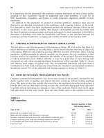
Perhaps the most common tools used in alignment are standard rulers or tape measures as
shown in Figure 6.1. The tape measure is typically used to measure the distances between
machinery hold down bolts (commonly referred to as the machinery ‘‘feet’’) and the points of
measurement on the shafts or coupling hubs. Graduations on tape measures are usually as
small as 1=16 to 1=32 in. (1 mm on metric tapes), which is about the smallest dimensional
measurement capable of discerning by the unaided eye. A straightedge is often used to ‘‘rough
align’’ the units as shown in Figure 6.2.
6.2.2 FEELER AND TAPER GAUGES
Feeler gauges are simply strips of metal shim stock arranged in a ‘‘foldout fan’’-type of
package design. They are used to measure soft foot gap clearances, closely spaced shaft end to
shaft end distances, rolling element to raceway bearing clearances, and a host of similar tasks
where fairly precise (+1 mil) measurements are required.
Taper gauges are precisely fabricated wedges of metal with lines scribed along the length of
the wedge that correspond to the thickness of the wedge at each particular scribe line. They
are typically used to measure closely spaced shaft end to shaft end distances where accuracy of
+10 mils is required.
FIGURE 6.1 Standard linear rulers.
Piotrowski / Shaft Alignment Handbook, Third Edition DK4322_C006 Final Proof page 221 26.9.2006 8:51pm
Shaft Alignment Measuring Tools 221
Looks straight enough for
me Melvin. Button it up and
let’s get back to the shop
The “calibrated eyeball”
Straightedge

Taper or feeler gauges
Taper gauge
Feeler gauge
FIGURE 6.2 Rough alignment methods using straightedges, feeler gauges, or taper gauges.
FIGURE 6.3 Misalignment visible by eye.
Piotrowski / Shaft Alignment Handbook, Third Edition DK4322_C006 Final Proof page 222 26.9.2006 8:51pm
222 Shaft Alignment Handbook, Third Edition
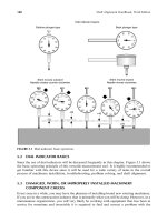
6.2.3 SLIDE CALIPER
The slide caliper has been used to measure distances with an accuracy of 1 mil (0.001 in.) for
the last 400 years. It can be used to measure virtually any linear distance such as shim pack
thickness, shaft outside diameters, coupling hub hole bores, etc. A very ingenious device has
been invented to measure shaft positional changes, whereas machinery is running utilizing
miniature slide calipers attached to a flexible coupling that will be reviewed in Chapter 16.
The primary scale looks like a standard ruler with divisions marked along the scale at
increments of 0.025 in. The secondary, or sliding scale, has a series of 25 equally spaced
marks where the distance from the first to the last mark on the sliding scale is 1.250 in. apart.
The jaws are positioned to measure a dimension by translating the sliding scale along the
length of the primary scale as shown in Figure 6.4. The dimension is then obtained by:
1. Observing where the position of the zero mark on the sliding scale is aligning between
two 25-mil division marks on the primary scale. A mental (or written) record of the
smaller of the two 25-mil division marks is made.
2. Observing which one of the 25 marks on the secondary scale aligns most evenly with
another mark on the primary scale. The value of the aligned pair mark on the secondary
scale is added with the recorded 25-mil mark in step 1.
Some modern slide calipers as shown in Figure 6.4 have a dial gauge incorporated into the
device. The dial has a range of 100 mils and is attached to the sliding scale via a rack and
pinion gear set. This eliminates the need to visually discern which paired lines match exactly
(as discussed in step 2 above) and a direct reading can then be made by observing the inch and
tenths of an inch mark on the primary scale, and then adding the measurement from the
indicator (Figure 6.5). With care and practice, measurement to +0.001 in. can be made with

either style.
6.2.4 MICROMETERS
Although the micrometer was originally invented by William Gascoigne in 1639, its use did
not become widespread until 150 years later when Henry Maudslay invented a lathe capable
of accurately and repeatably cutting threads. That of course brought about the problem of
how threads should be cut (number of threads per unit length, thread angles, thread depth,
FIGURE 6.4 Feeler gauges, slide caliper, and outside micrometer.
Piotrowski / Shaft Alignment Handbook, Third Edition DK4322_C006 Final Proof page 223 26.9.2006 8:51pm
Shaft Alignment Measuring Tools 223
etc.), which forced the emergence of thread standards in the Whitworth system (principally
abandoned) and the current English and metric standards.
The micrometer is still in prevalent use today and newer designs have been outfitted with
electronic sensors and digital readouts. The micrometer is typically used to measure shaft
diameters, hole bores, shim or plate thickness, and is a highly recommended tool for the
person performing alignment jobs.
A mechanical outside micrometer consists of a spindle attached to a rotating thimble,
which has 25 equally spaced numbered divisions scribed around the perimeter of the
thimble for English measurement system as shown in Figure 6.6. When the spindle touches
the mechanical stop at the tip of the C-shaped frame, the zero mark on the thimble of the
micrometer aligns with the sleeve’s stationary scale reference axis. As the thimble is rotated
and the spindle begins to move away from the mechanical stop, the precisely cut threads (40
threads=in.) insure that as the drum is rotated exactly one revolution, the spindle has moved
25 mils (1=40th of an inch or 0.025 in.). As the thimble continues to rotate, increasing the
distance from the spindle tip to the mechanical stop (anvil), the end of the thimble wheel
exposes division marks on the sleeve’s stationary scale scribed in 25-mil increments. Once the
1
0
23456789
1
1

23456789
2
0 5 10 15 20 25
Measure inside
dimensions here
Measure outside
dimensions here
Start here
Notice that the “zero” mark is
between 0.750 in. and 0.775 in.
Then find the mark on the thousandths scale
that lines up the best with one of the marks
on the ruler. In this case, it looks like the 6
thousandths lines up best with one of the
marks on the ruler, so the reading is
0.756 in.
Thousandths scale
Ruler
Note : This device was invented b
y
Pierre Vernier (France) around 1630 AD.
FIGURE 6.5 How to read a slide caliper.
01234567
0
5
Spindle
Thimble
Frame
Reading = 0.728 in.
Sleeve

FIGURE 6.6 How to read a micrometer.
Piotrowski / Shaft Alignment Handbook, Third Edition DK4322_C006 Final Proof page 224 26.9.2006 8:51pm
224 Shaft Alignment Handbook, Third Edition
desired distance between the anvil and the spindle is obtained, observe what 25-mil division
on the stationary scale has been exposed, then add whatever scribed division on the drum
aligns with the reference axis of the stationary scale.
6.2.5 DIAL INDICATORS
The dial indicator came from the work of a nineteenth century watchmaker in New England.
John Logan of Waltham, Massachusetts, filed a U.S. patent application on May 15, 1883 for
what he termed as ‘‘an improvement in gages.’’ Its outward appearance was no different than
the dial indicators of today but the pointer (indicator needle) was actuated by an internal
mechanism consisting of a watch chain wound around a drum (arbor). The arbor diameter
determined the amplification factor of the indicator. Later, Logan developed a rack and
pinion assembly that is currently in use today on most mechanical dial indicators.
The full range of applications of this device was not recognized for another 13 years when
one of Logan’s associates, Frank Randall, another watchmaker from E. Howard Watch Co.,
Boston, bought the patent rights from Logan in 1896. He then formed a partnership with
Francis Stickney and began manufacturing dial indicators for industrial use. A few years later
B.C. Ames also began manufacturing dial indicators for general industry.
The German professor Ernst Abbe established the measuring instrument department at the
Zeiss Works in 1890 and by 1904 he had developed a number of instruments, which included a
dial indicator, for sale to industry. The basic operating principle of dial indicator was
discussed in Chapter 5 (see Figure 5.1). The dial indicator is still in prevalent use today and
newer designs have been outfitted with electronic sensors and digital readouts.
For the past 50 years, the most common tool that has been used to accurately measure shaft
misalignment is the dial indicator as shown in Figures 6.7 through Figures 6.9. There are
some undeniable benefits of using a dial indicator for alignment purposes:
.
One of the preliminary steps of alignment is to measure runout on shafts and coupling
hubs to insure that eccentricity amounts are not excessive. As we have seen in Chapter 5,

the dial indicator is the measuring tool typically used for this task and is therefore usually
one of the tools that the alignment expert will bring to an alignment job. Since a dial
indicator is used to measure runout, why not use it also to measure the shaft centerline
positions?
.
The operating range of dial indicators far exceeds the range of many other types of
sensors used for alignment. Dial indicators with total stem travels of 0.200 in. (5 mm) are
traditionally used for alignment but indicators with stem travels of 3 in. or greater could
also be used if the misalignment condition is moderate to severe when you first begin to
‘‘rough in’’ the machinery.
.
The cost of a dial indicator (around US$70 to US$110) is far less expensive than many of
the other sensors used for alignment. You could purchase over 140 dial indicators for the
average cost of some other alignment tools currently on the market.
.
Since the dial indicator is a mechanically based measurement tool, there is a direct visual
indication of the measurement as you watch the needle rotate.
.
They are very easy to test for defective operation.
.
They are much easier to find and replace in virtually every geographical location on the
globe in the event that you damage or lose the indicator.
.
Batteries are not needed.
.
The rated measurement accuracy is equivalent to the level of correction capability
(i.e., shim stock cannot be purchased in thickness less than 1 mil)
Piotrowski / Shaft Alignment Handbook, Third Edition DK4322_C006 Final Proof page 225 26.9.2006 8:51pm
Shaft Alignment Measuring Tools 225
6.2.6 OPTICAL ALIGNMENT TOOLING

Optical alignment tooling consists of devices that combine low-power telescopes with accur-
ate bubble levels and optical micrometers for use in determining precise elevations (horizontal
planes through space) or plumb lines (vertical planes through space). They are not to be
confused with theodolite systems that can also measure the angular pitch of the line of sight.
They are similar to surveying equipment but with much higher measurement accuracies.
Optical alignment systems are perhaps one of the most versatile tools available for a wide
variety of applications such as leveling foundations (e.g., see Figure 3.11), measuring OL2R
machinery movement (covered in Chapter 16), checking for roll parallelism in paper and steel
FIGURE 6.7 Dial indicator.
FIGURE 6.8 Dial indicator taking rim measurement on steam turbine shaft with bracket clamped onto
end of compressor shaft.
Piotrowski / Shaft Alignment Handbook, Third Edition DK4322_C006 Final Proof page 226 26.9.2006 8:51pm
226 Shaft Alignment Handbook, Third Edition
manufacturing plants, aligning bores of cylindrical objects such as bearings or extruders,
measuring flatness or surface profiles, checking for squareness on machine tools or frames,
and will be discussed in Chapter 19. If you have a considerable amount of rotating machinery
in your plant, it is highly recommended that someone examine all the potential applications
for this extremely useful and accurate tooling.
Optical tooling levels and jig transits are one of the most versatile measurement systems
available to determine rotating equipment movement. Figure 6.10 and Figure 6.11 show the
FIGURE 6.9 Dial indicator and bracket arrangement taking rim reading on a large flywheel.
FIGURE 6.10 Optical tilting level and jig transit.
Piotrowski / Shaft Alignment Handbook, Third Edition DK4322_C006 Final Proof page 227 26.9.2006 8:51pm
Shaft Alignment Measuring Tools 227
two most widely used optical instruments for machinery alignment. This tooling is extremely
useful for leveling foundations, squaring frames, checking roll parallelism, and a plethora of
other tasks involved in level, squareness, flatness, vertical straightness, etc.
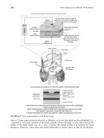
The detail of a 3 in. scale target is shown in Figure 6.12. Optical scale targets can be
purchased in a variety of standard lengths (3, 5, 10, 20, and 40 in.) and metric scales are
available. The scale pattern is painted on invar bars to minimize thermal expansion or

contraction of the scale target itself. The scale targets are held in position with magnetic
base holders as shown in Figure 6.13 and Figure 6.14.
There are generally four sets of paired line sighting marks on the scales for centering of the
crosshairs when viewing through the scope as shown in Figure 6.12. An optical micrometer,
as shown in Figure 6.15, is attached to the end of the telescope barrel and can be positioned in
either the horizontal or vertical direction. The micrometer adjustment wheel is used to align
the crosshairs between the paired lines on the targets. When the micrometer wheel is
rotated, the crosshair appears to move up and down along the scale target (or side to side
FIGURE 6.11 Jig transit. (Courtesy of Brunson Instrument Co., Kansas City, MO. With permission.)
Piotrowski / Shaft Alignment Handbook, Third Edition DK4322_C006 Final Proof page 228 26.9.2006 8:51pm
228 Shaft Alignment Handbook, Third Edition
depending on the positionofthemicrometer). Oncethecrosshair islinedupbetweenaset ofpaired
lines, a reading is taken based on where the crosshair is sighted on the scale and the position of the
optical micrometer. The inch and tenths of an inch reading is visually taken by observing the scale
target number where the crosshair aligns between a paired line set, and the hundredth and
thousandths of an inch reading is taken on the micrometer drum as shown in Figure 6.16.
The extreme accuracy (one part in 200,000 or 0.001 in. at a distance of 200 in.) of the optical
instrument is obtained by accurately leveling the scope using the split coincidence level
mounted on the telescope barrel as shown in Figure 6.17.
6.2.7 OPTICAL PARALLAX
As opposed to binoculars, 35 mm cameras, and microscopes that have one focusing adjust-
ment, the optical scope has two focusing knobs. There is one knob used for obtaining a clear,
sharp image of an object (e.g., the scale target) and another adjustment knob that is used to
focus the crosshairs (reticle pattern). Since your eye can also change focus, adjust both these
knobs so that your eye is relaxed when the object image and the superimposed crosshair
image are focused on a target.
Adjusting the focusing knobs:
1. With your eye relaxed, aim at a plain white object at the same distance away as your
scale target and adjust the eyepiece until the crosshair image is sharp.
2. Aim at the scale target and adjust the focus of the telescope.

3. Move your eye slightly sideways and then up and down to see if there is an apparent
motion between the crosshairs and the target you are sighting. If so, defocus the telescope
and adjust the eyepiece to refocus the object. Continue alternately adjusting the tele-
scope focus and the eyepiece to eliminate this apparent motion.
Before using any optical instrument, it is highly recommended that a Peg Test be per-
formed. The Peg Test is a check on the accuracy of the levelness of the instrument. Figure 6.18
shows how to perform the Peg Test.
Figure 6.19 and Figure 6.20 show the basic procedure on how to properly level the
instrument. If there is any change in the split coincidence level bubble gap during the final
check, go back and perform this level adjustment again. This might take a half an hour to an
hour to get this right, but it is time well spent. It is also wise to walk away from the scope for
about 30 min to determine if the location of the instrument is stable and to allow some time
123
2468 2468 2468
Optical
scale
target
0.060 in. gap between marks for sights from 50 to 130 ft
0.010 in. gap between marks for sights from 7 to 20 ft
0.004 in. gap between marks for sights up to about 7 ft
0.025 in. gap between marks for sights from 20 to 50 ft
FIGURE 6.12 Three inch optical scale target.
Piotrowski / Shaft Alignment Handbook, Third Edition DK4322_C006 Final Proof page 229 26.9.2006 8:51pm
Shaft Alignment Measuring Tools 229
FIGURE 6.13 Scale targets mounted on an electric generator bearing.
Piotrowski / Shaft Alignment Handbook, Third Edition DK4322_C006 Final Proof page 230 26.9.2006 8:51pm
230 Shaft Alignment Handbook, Third Edition
FIGURE 6.14 Scale targets mounted on compressor casing near their centerline of rotation.
FIGURE 6.15 An optical micrometer. (Courtesy of Brunson Instrument Co., Kansas City, MO. With
permission.)

Piotrowski / Shaft Alignment Handbook, Third Edition DK4322_C006 Final Proof page 231 26.9.2006 8:51pm
Shaft Alignment Measuring Tools 231
for your eyes to uncross. If the split coincidence bubble has shifted during your absence, start
looking for problems with the stand or what it is sitting on. Correct the problems and relevel
the scope.
I cannot overemphasize the delicacy of this operation and this equipment. It is no place for
people in a big hurry with little patience. If you take your time and are careful and attentive
when obtaining your readings, the accuracy of this equipment will astonish you.
6.2.8 PROXIMITY PROBES
Proximity probes (also known as inductive pickups) as shown in Figure 6.21 and Figure 6.22
are basically noncontacting, electronic dial indicators. They are devices used to measure
distance from the tip of the probe to a conductive surface. They are typically used to
measure vibration (i.e., shaft motion) or thrust position and are usually permanently mounted
to the machine. When used to measure vibration, the alternating current (AC) voltage from
the probe is measured. When used to measure distance, the direct current (DC) voltage is
measured.
Although the probes have been proposed for use as shaft alignment measuring devices, no
company currently offers such a system for sale. Proximity probes can also be used to
Crosshair when
viewing through
scope barrel
Optical micrometer
Instrument lens
Plate glass with near
perfect parallel sides
When optical micrometer barrel is rotated, the glass
pivots making it appear that the horizontal cross
hair is moving up or down on the scale target
Notice in the upper drawing that when the optical micrometer is in
zero position, the horizontal crosshair is between 2.6 and 2.7 on

scale target but the crosshair is not exactly aligned with any of
marks. By rotating the micrometer drum, the horizontal
crosshair is aligned at the 2.6 mark on the scale target. The inch
and tenths of an inch reading is obtained off the scale target, the
hundredths and thousandths of an inch reading is obtained off the
micrometer drum position.The final readin
g
above is 2.643.
10
10
5
5
0
10
10
0
10
10
5
5
0
30
50
40
60
Optical
scale
target
12
3

2468 2468
2468
12
3
2468 2468
2468
Optical
scale
target
FIGURE 6.16 Principle of an optical micrometer.
Piotrowski / Shaft Alignment Handbook, Third Edition DK4322_C006 Final Proof page 232 26.9.2006 8:51pm
232 Shaft Alignment Handbook, Third Edition
measure OL2R machinery movement in some very innovative ways as explained in
Chapter 16. Their primary limitation is the range of useful distance measurement (app-
roximately 50–150 mils) that can be attained with standard probes. Various sensitivities can
be attained depending on the construction of the probe. Proximity probes frequently used as
vibration sensors have either a 100 or 200 mV=mil sensitivity.
6.2.9 LINEAR VARIABLE DIFFERENTIAL TRANSFORMERS
These devices are also called variable inductance transducers. They output an AC signal
proportional to the position of a core that moves through the center of the transducer
as illustrated in Figure 6.23 and Figure 6.24. These devices can attain accuracies of +1%
of full-scale range with stroke ranges available from 20 mils to over 20 in. No current
(b)
Mirrors
Mirrors
FIGURE 6.17 Principle of the coincidence level. (Courtesy of Brunson Instrument Co., Kansas City,
MO. With permission.)
Piotrowski / Shaft Alignment Handbook, Third Edition DK4322_C006 Final Proof page 233 26.9.2006 8:51pm
Shaft Alignment Measuring Tools 233
3. Move the scope to the 1/5 L position, level the scope, and alternately

take four readings on scale target #1 (reading C) and scale target #2
(reading D). Record and average these readings.
4. If the instrument is calibrated, A minus B should equal C minus D (at
32 ft, this should be no more than 0.002 in.).
If the error is greater than that, adjust the split coincidence levels as
follows:
A. Set the optical micrometer drum to the hundreths and thousandths
value of E. For example, if E = 4.656, set the micrometer drum to 0.056.
B. Using the tilting screw, tilt the scope barrel to align the horizontal
crosshair to the inch and tenths of an inch mark on scale target #2. For
example, if E = 4.656, align the horizontal crosshair to the paired lines
at 4.6. At this point, the split coincidence level will be not be coincident.
C. Adjust the nuts holding the split coincident level to the scope barre
to bring the bubble halves into coincidence.
l
D. Perform step 1 through step 4 above to verify that the adjustment worked.
Should this not be the case, the coincidence level calibration adjustment
nuts can be adjusted to position the leveled line of sight to be set at
reading E.
1
2
3
4
5
1
2
3
4
5
C

D
E
Level line of sight
L/5
1
2
3
4
5
1
2
3
4
5
A
B
Scale target #1
L
L /2
The Peg Test
1. Set two scales apart by distance L (usually 40 ft) on stable
platforms. Position the optical telescope or transit exactly half way
between both scales. Accurately level the instrument using the split
coincidence level.
2. Alternately take four readings on scale target #1 (reading A) and
scale target #2 (reading B). Record and average these readings.
E = 4/3((B
+C )−(A +D )) + D
Before using any optical instrument, it is recommended that
the Peg Test be performed to insure measurement accuracy.

At 40 ft, the accuracy of the scope is plus or minus 0.0024 in.
Scale target #2
FIGURE 6.18 Coincidence level calibration test (the Peg Test).
Piotrowski / Shaft Alignment Handbook, Third Edition DK4322_C006 Final Proof page 234 26.9.2006 8:51pm
234 Shaft Alignment Handbook, Third Edition
manufacturer of alignment measurement systems uses this type of transducer for shaft
alignment purposes.
6.2.10 OPTICAL ENCODERS
Optical encoders are essentially pulse counters as shown in Figure 6.25. They are most
frequently used to measure shaft speed or shaft position and are therefore sometimes called
shaft or rotational encoders. A series of slots are etched on a disk or flat strip. A light source
(typically an light-emitting diode, LED) aims at the disk or flat strip and as the disk or strip is
moved or rotated, a photodetector on the other side of the disk or strip counts the number of
slots that are seen. One manufacturer currently uses this type of sensor for shaft alignment
measurement.
6.2.11 LASERS AND DETECTORS
With the advent of the microprocessor chip, the semiconductor junction laser, and silicon
photodiodes, new inroads have been forged in the process of measuring small distances that
utilize these new electronic devices instead of mechanical measuring instruments. Since the
1. Set the instrument stand at the
desired sighting location, attach the
alignment scope to the tripod or
instrument stand and level the
stand using the “rough” circular
bubble level on the tripods (if there
is one on the tripod). Insure that
the stand is steady and away from
heat sources, vibrating floors,
and curious people who may
want to use the scope to see sunspots.

2. Rotate the scope barrel to line up with two of the four leveling screws
and adjust these two leveling screws to roughly center the split
coincidence level bubble in the same tilt plane as the two screws that are
adjusted as shown. The two leveling screws should be snug but not
so tight as to warp the mounting frame.
3. Rotate the scope barrel 90Њ to line up with the other two
leveling screws to completely center the bubble in the circular level as
shown.
4. If the circular level is still not centered, repeat step 2 and step 3.
Adjust these two leveling screws to first
adjust the circular level in one direction
And then
these two
screws for the
other
direction
Split coincidence level
Circular level
Tilting screw
Leveling screws
How to level optical tilting levels and jig transits
10
10
5
5
0
30
50
40
60

10
10
5
5
0
30
50
40
60
FIGURE 6.19 How to level a tilting level or jig transit, part 1 through part 4.
Piotrowski / Shaft Alignment Handbook, Third Edition DK4322_C006 Final Proof page 235 26.9.2006 8:51pm
Shaft Alignment Measuring Tools 235
How to level optical tilting levels and jig transits
8. The last step is to rotate the scope barrel
90Њ to line up with the two remaining
leveling screws yet to be fine adjusted.
Follow the same procedure as outlined in
step 6 and step 7 above. When these
adjustments have been completed, the split
coincidence bubble should be coincident
when rotating the scope barrel through the
entire 360Њ of rotation around its
azimuth axis.
5. Once again rotate the scope
to line up with two of the
leveling screws as covered in
step 2. Adjust the tilting screw
to center the split coincidence
level on the side of the scope
barrel as shown.

6. Rotate the scope barrel 180Њ
and note the position of the two
bubble halves. Adjust the two
leveling screws in line with the
scope barrel so that the gap
between the two bubble halves is
exactly one half the original gap.
7. At this point, adjust the tilting screw so there
is no gap in the two bubble halves. Rotate the
scope barrel back 180Њ to its original
position and see if the two bubble halves are
still coincident (i.e., no gap). If they are not
adjust the two leveling screws and the tilting
level screw again as shown and rotate the scope
barrel back 180Њ until there is no gap
when swinging back and forth through the half
circle. Again, the two leveling screws should
be snug but not so tight as to warp the mounting
10
10
5
5
0
30
50
40
60
10
10
5

5
0
30
50
40
60
10
10
5
5
0
30
50
40
60
10
10
5
5
0
30
50
40
60
Gap
Half gap
No gap
Gap
Half gap
No gap

FIGURE 6.20 How to level a tilting level or jig transit, part 5 through part 8.
FIGURE 6.21 Proximity probe and oscillator–demodulator.
Piotrowski / Shaft Alignment Handbook, Third Edition DK4322_C006 Final Proof page 236 26.9.2006 8:51pm
236 Shaft Alignment Handbook, Third Edition
Gap variation
seen as
change in
DC output
voltage
“Donut”-shaped coil energized
by a radio frequency signal
from oscillator–demodulator
Magnetic field
Conductive tar
g
et
Typical target sensitivity is 100 or 200 mv/mil
FIGURE 6.22 Basic operation of a proximity probe.
FIGURE 6.23 LVDT sensor.
Core
Output voltage
Input voltage
Core position
Output voltage
FIGURE 6.24 Basic operation of an LVDT.
Piotrowski / Shaft Alignment Handbook, Third Edition DK4322_C006 Final Proof page 237 26.9.2006 8:51pm
Shaft Alignment Measuring Tools 237
first useable laser shaft alignment measurement system was introduced in Germany in 1984, a
host of manufacturers have introduced other laser shaft alignment systems. Since some of the
manufacturers have taken slightly different approaches for using lasers and detectors, it will

be beneficial to initially discuss some of the basic theory of operation of photonic semicon-
ductors and how they are applied to mechanical measurements.
Useful terms:
Photonics: Field of electronics that involves semiconductor devices that emit and detect light.
Semiconductors: Typically silicon crystal doped (i.e., made impure) with other elements such
as phosphorus (n-type due to five electrons in outer shell) or boron (p-type due to three
electrons in outer shell). Depending on certain conditions, semiconductors can act as insula-
tors or conductors.
LASER: Acronym for light amplified by stimulated emission of radiation.
LED: Acronym for light-emitting diode. All diodes emit some electromagnetic radiation when
forward biased. When the forward current attains a certain level, called the threshold point,
lasing action occurs in the semiconductor. Gallium–arsenide–phosphide diodes emit much
more radiation than silicon-type diodes and are typically used in semiconductor junction
diode lasers.
Photodiode: All diodes respond when subjected to light (electromagnetic radiation). Silicon
diodes respond very well to light and are typically used to detect the presence or position of
light as it impinges on the surface of the diode.
Figure 6.26 shows the broad frequency range of the electromagnetic spectrum. The human
eye can detect but a very small range of frequencies from 400 to 700 nm. Figure 6.27 illustrates
the basic operation of semiconductor junction laser diodes. As current is passed through the
diode, photons (light) are emitted in the junction region as electrons move from a higher
Photodetector
LED
Volta
g
e
Output
The photodetector senses when the light
is shining or not through the slots or
“windows.” With 4000 slots per inch, 1/2 mil

of resolution can be attained
FIGURE 6.25 Basic operation of an optical encoder.
Piotrowski / Shaft Alignment Handbook, Third Edition DK4322_C006 Final Proof page 238 26.9.2006 8:51pm
238 Shaft Alignment Handbook, Third Edition
orbital shell to a lower one, giving up energy in the form of quanta (photons) in the process.
By altering the chemical composition of the semiconductor, the wavelength of the light
emitted from the semiconductor can be shifted to different frequencies.
The first lasers used in shaft alignment measurement systems emitted light at a wavelength
of 760 nm, outside the visible range of human sight. The lasers currently used in alignment
now emit a red light (670 nm), which is within the visible range of human sight. The beam of
light that is emitted from the laser is not a thin strand of light 1 mm in diameter. Instead it is
10
Ϫ12
m
1 m 1000
m
10
Ϫ9
m10
Ϫ6
m10
Ϫ3
m
Picometer (pm) Nanometer (nm) Micrometer (µm) Millimeter (mm) Meter Kilometer
X-rays
Gamma rays
Ultraviolet Infrared
Microwave
Radio waves
Visible light

300 nm 400 nm 500 nm 600 nm 700 nm 800 nm
Violet
Blue
Green
Yellow
Orange
Red
Near infrared
Detectable
wavelengths of
the human eye
670 nm 760 nm
Visible
lasers
Invisible
lasers
Electromagnetic
spectrum
Electric field
Magnetic field
The two “faces” of electromagnetic energy
Energy “packets” of photons
The photon is the key behind controlling an atom’s orbital energy.
Absorption occurs when electrons go from a lower to a higher orbital level (shell).
Emission occurs when electrons
g
o from a hi
g
her to a lower orbital level.
FIGURE 6.26 (See color insert following page 322.) The electromagnetic spectrum.

Piotrowski / Shaft Alignment Handbook, Third Edition DK4322_C006 Final Proof page 239 26.9.2006 8:51pm
Shaft Alignment Measuring Tools 239
about 1.5 mm (approximately 60 mils) in diameter as it exits the diode and is collimated (i.e.,
‘‘focused’’), since only one side of the diode actually allows the light to exit. After exiting the
diode, if the light beam was in a pure vacuum, the beam would stay focused for long
distances. However, since there are small molecules of water vapor in the air we breathe,
How semiconductor junction diode lasers work
Battery
positive (+)
Battery
negative (−)
n-Type
semiconductor
Current must be high enough for
electrons to move from a higher to a
lower energy level in the junction
p-Type
semiconductor
Hole+
Hole+
Electron-
Electron
-
Junction
Partially reflective facets
on both sides of the
edge of the “chip” act as
an optical resonance
chamber
Battery

Photon
Photon
Photon
Photon
Collimated light beam
Glass lens
Cap
Heat sink
Laser diode
Monitor PIN
photodiode
Stem
Laser “beam”
• The chemical composition of the semiconductor determines the wavelength
of light emitted from the laser.
• Near infrared lasers used for alignment measurement devices are made
from gallium–aluminum–arsenide (620–895 nm).
• Visible red lasers are made from
g
allium–indium–phosphorous (670 nm).
Cross-sectional structure of a 670 nm GaInP semiconductor laser
p-GaAs (cap layer)
n-GaAs (backing)
p-(Ga
1−x
Al
x
)
0.5
I

0.5
P
Ga
0.5
I
0.5
P
n-(Ga
1−x
Al
x
)
0.5
I
0.5
P
GaAs
n-GaAs substrate
Confining layer
Active layer
Buffer layer
Confining layer
FIGURE 6.27 How semiconductor laser diodes work.
Piotrowski / Shaft Alignment Handbook, Third Edition DK4322_C006 Final Proof page 240 26.9.2006 8:51pm
240 Shaft Alignment Handbook, Third Edition
the light from the laser is diffracted as it passes through each molecule of water vapor
diffusing the beam. Typically, the useable distance of laser is somewhat limited to 30 ft due
to the diffraction of the beam. Since the laser beam is around 60 mils in diameter as it exits the
diode, the measurement accuracy would only be 60 mils (i.e., about 1=16th of an inch) if just
the laser beam were solely used as the measurement device. This accuracy is just fine for laser

levels when constructing buildings, for example, but since we are looking for accuracies of
measurement at 1 mil or better, another device is needed in concert with the laser to attain this
measurement precision. That device is the beam detector target.
Laser–detector systems are also semiconductor photodiodes capable of detecting electro-
magnetic radiation (light) from 350 to 1100 nm. When light within this range of wavelengths
strikes the surface of the photodiode, an electrical current is produced as shown in Figure 6.28.
Since the laser beam is emitting light at a specific wavelength (e.g., 670 nm), a colored
translucent filter is positioned in front of the diode target to hopefully allow only light in
the laser’s wavelength to enter. Otherwise, the detector could not tell whether the light that
was striking its surface was from the laser, overhead building lighting, a flashlight, or the sun.
As shown in Figure 6.29, when light strikes the center of the detector, output currents from
each cell are equal. As the beam moves across the surface of the photodiode, a current
imbalance occurs, indicating the off-center position of the beam. Most manufacturers of
laser–detector shaft alignment systems use 10 Â 10 mm detectors (approximately 3=8 sq. in.);
a few may use 20 Â 20 mm detectors. Some manufacturers of these systems use bicell
(unidirectional) or quadrant cell (bidirectional) photodiodes to detect the position of the
laser beam. An unidirectional photodiode measures the beam position within the target area
from left to right only whereas a bidirectional photodiode (Figure 6.30 and Figure 6.31)
measures the beam position in both axes, left to right and top to bottom. Therefore, laser–
detector systems measure the distance the laser beam has traversed across the surface of
the detector by measuring the electrical current at the beam’s starting position and the
electrical current at the beam’s finishing position.
6.2.12 CHARGE COUPLE DEVICES
The CCD was originally proposed by Boyle and Smith in 1970 as an electrical equivalent to
magnetic bubble digital storage devices. The basic principle of their device was to store
information in the form of electrical ‘‘charge packets’’ in potential wells created in the
semiconductor by the influence of overlying electrodes separated from the semiconductor
Cathode
Anode
CathodeAnode

Photodetector
Actual size
20 ϫ 20 mm 10 ϫ 10 mm
FIGURE 6.28 How photodiodes work.
Piotrowski / Shaft Alignment Handbook, Third Edition DK4322_C006 Final Proof page 241 26.9.2006 8:51pm
Shaft Alignment Measuring Tools 241
by a thin-insulating layer. By controlling voltages applied to the electrodes, the potential wells
and hence the charge packets could be shifted through the semiconductor (Figure 6.32).
The potential wells are capable of storing variable amounts of charge and can be intro-
duced electrically or optically. Light impinging on the surface of the charge-coupled semi-
conductor generates charge carriers, which can be collected in the potential wells and
afterward clocked out of the structure enabling the CCD to act as an image sensor.
Laser
Detector
Cathode
Anode
CathodeAnode
Laser beam
(1.5 ϫ 1.5 mm)
Differential current measured across anode and
cathode pins to determine beam position
FIGURE 6.29 Laser–photodiode operation.
−
+
−
+
−
+
−
+

Numerator
Denominator
Divider
R
2
R
3
R
1
Transimpedance
amplifier
Difference
amplifier
Sum amplifier
Transimpedance
amplifier
R
1
R
2
R
2
R
3
0.1 µF
15 V
∆X
L /2
R
2

FIGURE 6.30 Typical single axis photodiode circuit.
Piotrowski / Shaft Alignment Handbook, Third Edition DK4322_C006 Final Proof page 242 26.9.2006 8:51pm
242 Shaft Alignment Handbook, Third Edition
A considerable amount of effort was put forth in the 1960s in developing optical imagers
that utilized matrices of photodiodes that effectively became undone by the development of
the CCD. The rate of progress in CCD design through 1974 was so astonishing that Rodgers
demonstrated a 320Â512 bit CCD sensor that could be used for 525 line television imaging
just 4 years after the CCD was invented. CCDs have found their way into everyday life in
video cameras and in high technology fields such as astronomy where large area CCDs
capture images in telescopes both in orbit and on Earth.
With the recent pace of introducing electronic measurement sensors in the arena of
alignment, it seems odd that no one has incorporated the CCD as a measurement sensor.
The only known application of CCDs for use in alignment was presented as a doctoral thesis
by Brad Carman and a research project at the University of Calgary (see references).
6.2.13 INTERFEROMETERS
It is suggested that one has to study Figure 2.10 through Figure 2.12 to get a basic under-
standing of amplitude and frequency. Although the discussion in Chapter 2 for these figures
∆X
L /2
∆X
L /2
−
−
−
−
−
−
−
+
+

+
Numerator
Denominator
Divider
R
2
R
3
R
1
Difference
amplifier
R
1
R
2
+
+
+
+
Numerator
Denominator
Divider
R
2
R
3
R
1
Difference

amplifier
Sum amplifier
R
1
R
2
R
2
R
2
R
3
R
2
V+
V−
0.1 µF
0.1 µF
Anode
Bias
adjustment
Bias adjustment
FIGURE 6.31 Typical dual axis photodiode circuit.
Piotrowski / Shaft Alignment Handbook, Third Edition DK4322_C006 Final Proof page 243 26.9.2006 8:51pm
Shaft Alignment Measuring Tools 243
centers around vibration, the same principles can also be applied to sound or light. Also
Figure 6.26 explains the electromagnetic spectrum.
Interferometers are instruments that utilize monochromatic (i.e., single wavelength) beams
of light to measure distance by utilizing the principle of interference of waves. When two
signals of the same frequency combine and are in phase, the amplitude of the combined signal

intensifies. However, when two signals of the same frequency combine and are exactly 1808
out of phase, the two signals cancel each other out. This is referred to as constructive or
destructive interference and is the basis of the field of interferometry. Since the wavelength of
light is very small, small amounts of distance can be measured very accurately with these
devices. Linear resolutions of 0.0059 min. (0.15 nm) and angular resolutions of 0.005 arc
seconds can be measured with these systems. Not only can these systems measure distance,
but using the Doppler effect, they can also measure the speed of the object. Distance
measuring interferometers work on two principles:
1. Homodyne interferometers count fringes. A fringe is defined as one full cycle of light
variation, that is, from light to dark and back to light again, a full 3608 phase shift in the
two signals.
2. Heterodyne interferometers measure the change in optical phase of the known frequency
of a reference signal to the known, but different frequency of a measurement signal at
defined time intervals.
Although interferometers are not used in the area of shaft alignment, they are frequently used
in the field of metrology. Figure 6.34 shows the basic operating principles of a Michelson
interferometer.
Electrons
A CCD is a multilayered silicon chip. In one layer, an array of
electrodes divides the surface into pixels. Each electrode is
connected to leads, which carry a voltage. The image forms on
the silicon substrate. Light particles pass through the CCD
freeing electrons in the silicon substrate. The voltage applied to
the leads draws freed electrons together in special areas in the
silicon substrate, called photo sites. The number of gathering
electrons at the photo site is dependent on the intensity of the
light striking in that area. The CCD transfers captured electrons,
one by one, to an analog to digital converter, which assigns each
site a digital value corresponding to the number of electrons a
site holds. The number of electrons at each site determines how

light or dark each pixel in the image is.
Photo site
Electrode
Silicon
substrate
Lead
Electrode
layer
CCD
FIGURE 6.32 How a charge-coupled device (CCD) works.
Piotrowski / Shaft Alignment Handbook, Third Edition DK4322_C006 Final Proof page 244 26.9.2006 8:51pm
244 Shaft Alignment Handbook, Third Edition