Handbook of Shaft Alignment Part 8 potx

many more that are logical, easy, and inexpensive to do. If your alignment system limits you
to a few choices, there is a possibility that you will eventually run into trouble. Honestly, if
you do enough alignment jobs, I can virtually guarantee, you will run into a problem with a
limited number of solutions. To my knowledge, there is no more effective way to correct
misalignment than the methodology explained in this chapter.
Still today, some people who align rotating equipment will do trial-and-error alignment. They
install some shim stock under the feet and move the machinery sideways a little bit, take another
set of readings, and see if the measurements got any better. This sophisticated technique called
guessing will eventually produce frustration, anxiety, and anger if continued for long periods of
time. To a certain extent I applaud their effort. At least they made an attempt to improve the
misalignment condition; many others do not even try. There happens to be a much better way to
determine how to accurately position the machinery instead of guessing. And there happens to be
a better way than having a limited computer software program telling you what to do, particu-
larly if there could be a simpler way to solve the misalignment condition.
Even for people who align rotating machinery on a regular basis, it is very difficult to
visualize exactly where the centerlines of rotation are by just looking at dial indicator, laser, or
optical encoder measurement data. Your goal is to position each machine so that both shafts
FIGURE 8.1 Representing the centerlines of rotation of machinery shafts as straight lines.
Piotrowski / Shaft Alignment Handbook, Third Edition DK4322_C008 Final Proof page 320 6.10.2006 12:13am
320 Shaft Alignment Handbook, Third Edition
run in the same axis of rotation and you invariably begin to wonder—Is one shaft higher or
lower than the other one, is it to the west or is it to the east, and if so, how much?
Alignment models can be as simple or as complex as the drive system itself. If you are trying
to align two pieces of machinery such as a motor and a pump, the alignment model can be
constructed to show both of those shafts. If you are trying to align an eight-element drive
system with a right angle in the drive, the alignment model can be constructed to show every
one of the shafts including the right angle turn the drive system makes. This chapter is
intended to introduce you to modeling a two-element drive system. More complex drive
systems are covered in Chapter 16 and Chapter 17.
8.1 GRAPHING AND MODELING ALIGNMENT TECHNIQUES
Regardless of the device used to measure the positions of the centerlines of rotation (be it dial

indicators, optical encoders, lasers, and the like), virtually every alignment measurement
system utilizes one (or a slight variation) of the following measurement approaches:
1. Reverse indicator method (Chapter 10)
2. Face and rim method (Chapter 11)
3. Double radial method (Chapter 12)
4. Shaft to coupling spool method (Chapter 13)
5. Face–face method (Chapter 14)
To understand how each of these techniques work, dial indicator readings will be used to
illustrate how each method can be graphed or modeled to determine the relative positions of
each shaft. All of these techniques can be graphed or modeled by hand. Typically all you need
is some graph paper (20 division=in. is a good choice), a straightedge, and a pencil (with an
eraser just in case). You do not even really need graph paper; all that is required is a scaled
grid or some sort of measurement device like a ruler, but graph paper helps.
8.2 BASIC ALIGNMENT MODELS
The graphical shaft alignment modeling techniques use two different scaling factors. One
scaling factor proportions the overall dimensions of the machinery drive system to fit within
the boundaries of the graph paper and another different scaling factor is used to exaggerate
the misalignment between the machinery shafts.
If we limit our discussion to horizontally mounted rotating machinery drive trains for now,
there will be two graphs that need to be drawn. As depicted in Figure 8.2, one graph will show
the exaggerated positions of each shaft in the side view illustrating the up and down or vertical
positions of the machinery. Another graph will be constructed in the top view that will
illustrate the side-to-side or lateral positions of the machinery. Figure 8.3 shows a three-
dimensional view of the drive system misalignment.
Keep in mind that the shaft centerline positions shown in the side and the top views are
exaggerated to help visualize the misalignment condition. Once the relative positions of the
machinery shafts are constructed on the graph, a wide variety of different solutions can be
determined to bring the centerlines of rotation in line with each other. The benefit of modeling
rotating machinery is to visually represent an exaggerated, but accurately scaled picture of the
misalignment condition so you can easily ascertain what positions the machinery could be

moved that would make it easy to align the shafts within the boundary conditions imposed by
the baseplate or foundation and the allowable lateral restrictions between the machinery
casing bolts and the holes drilled in the machine cases (a.k.a. ‘‘bolt bound’’ conditions).
Piotrowski / Shaft Alignment Handbook, Third Edition DK4322_C008 Final Proof page 321 6.10.2006 12:13am
Alignment Modeling Basics 321
Additionally the modeling technique can include other measurement parameters such as
improperly fit piping, air gap clearances between stators and armatures, and fan rotor to
shroud clearances, for example. Finally, the graph is a permanent record of the alignment of
the machinery and can be kept for future reference.
In summary, this chapter will review the following key steps in correcting the misalignment
situation (refer to Step 6 in Chapter 1):
1. Determine the current positions of the centerlines of rotation of all the machinery.
2. Observe any movement restrictions on the machines at the control and adjustment
points (usually the machinery feet and hold down bolts).
3. Plot the restrictions on the graph or the model.
Side view
Top view
East
Scale:
4 in.
10 mils
Scale:
4 in.
10 mils
Up
FIGURE 8.2 Side and top view alignment models showing an exaggerated misalignment condition
between the two shafts in the vertical direction (side view) and in the lateral direction (top view).
Piotrowski / Shaft Alignment Handbook, Third Edition DK4322_C008 Final Proof page 322 6.10.2006 12:13am
322 Shaft Alignment Handbook, Third Edition
4. Determine the moves for either or both of the machinery casings on the graph or the

model that will be feasible to perform.
We will first begin by illustrating the basic principles of how to construct the relative
positions of the two centerlines of rotation and then show how you can determine the wide
variety of movement options available to you when repositioning misaligned machinery.
8.3 SCALING THE DRIVE SYSTEM ONTO THE ALIGNMENT MODEL
There are several key positions on your drive system where distances need to be measured for
scaling onto the graph paper. The most important ones are
Top view
Scale:
Scale:
4 in.
10 mils
4 in.
10 mils
east
Side view
up
FIGURE 8.3 (See color insert following page 322.) Three-dimensional view of the side and top views.
Piotrowski / Shaft Alignment Handbook, Third Edition DK4322_C008 Final Proof page 323 6.10.2006 12:13am
Alignment Modeling Basics 323
1. Where the foot and the hold down bolts are located on each machine
2. Where the measurements are taken on the machinery shafts
Other critical dimensions that may need to be taken are
1. Where measurements have been taken to observe how the machinery moved from off-
line to running conditions (refer to Chapter 16)
2. Where the piping connections are made
3. Where lateral adjustments are made (assuming they are not exactly where the foot bolts
are located)
4. Internal clearances between rotating and stationary components in each machine
To begin modeling your alignment problem, the drive system is scaled onto the graph as

shown in Figure 8.4 and Figure 8.5. The distances you measure along the length of the drive
train should be accurate within 1=4’’ if possible or at least with an accuracy of +1% of the
overall length of the drive system.
Motor Pump
15Љ 5.5Љ 7Љ 14.5Љ
Up
PumpSide viewMotor
10Љ
15Љ
Scale: 5Љ
5.5Љ 7Љ 14.5Љ10Љ
FIGURE 8.4 Scaling the machinery feet and measurement positions onto the graph.
Piotrowski / Shaft Alignment Handbook, Third Edition DK4322_C008 Final Proof page 324 6.10.2006 12:13am
324 Shaft Alignment Handbook, Third Edition
8.4 CARDINAL ALIGNMENT GRAPHING AND MODELING RULES
Alignment modeling can be confusing when you first attempt it but there are a few rules that
apply when constructing an alignment model using any of the alignment measurement methods:
1. Only plot measurements that have been compensated for bracket sag.
2. Only plot half of a rim dial indicator reading.
3. Positive (þ) dial indicator readings means the shaft is ‘‘low.’’
4. Negative (À) dial indicator readings means the shaft is ‘‘high.’’
5. Zero the indicator on the side that is pointing toward the top of the graph paper.
6. Whatever shaft the dial indicator (or any other measuring device) is taking readings on is
the shaft that you want to draw on the graph paper.
7. Superimpose your boundary conditions.
8. Select an alignment correction line (a.k.a. overlay line or final desired alignment line)
that is possible and easy to do.
8.4.1 PLOT MEASUREMENTS THAT HAVE BEEN COMPENSATED FOR BRACKET SAG
As discussed in Chapter 6, gravity will have an effect on a mechanical bracket when
measuring shaft positions on horizontally mounted machinery. Bracket sag typically only

Side view
Label which view you
are looking at and the
direction pointing to the
top of the graph paper.
Label where each
machine is located.
Mark down the
scale factor from
left to ri
g
ht.
You could use an X to
indicate where the center
of the bolts are located.
15Љ
5ЉScale:
5.5Љ 7Љ 10.25Љ 14.5Љ
Motor Pump
Up
FIGURE 8.5 Scaling the machinery feet and measurement positions onto the graph. Accurately scale off
the distances between the inboard and outboard feet of both machines, the distances from the inboard
feet of both units to the point where the dial indicator plungers are touching (i.e., taking readings) on
both shafts, and the distances between measurement points along the graph centerline from left to right.
Piotrowski / Shaft Alignment Handbook, Third Edition DK4322_C008 Final Proof page 325 6.10.2006 12:13am
Alignment Modeling Basics 325
affects the measurements taken from the top to the bottom of a shaft and will come into play
when plotting the shafts in the side view alignment model. Usually the amount of bracket sag
is the same on both sides of a shaft and therefore the sags cancel each other out. The readings
taken from one side of a shaft to the other side are plotted in the top view alignment model. If

you are not sure how to compensate for bracket sag in your measurements, review the section
in Chapter 6 and specifically Figure 6.56 and Figure 6.57.
8.4.2 RIM READINGS ARE ALWAYS TWICE THE OFFSET AMOUNT
Remember, anytime a rim or circumferential reading is taken, the amount measured from one
side to the other side of the shaft (1808 of rotation) is twice the amount of the actual distance
between the centerlines of rotation at that point. Refer to Figure 6.44 and Figure 6.45 to
understand why this happens.
8.4.3 PLUS MEANS ‘‘LOW’’ AND MINUS MEANS ‘‘HIGH’’
Where and how to position the rotating machinery shafts on the alignment model will make
far more sense if you reason out what the measurement sensor has told you. If you zero a dial
indicator at the top of a shaft, sweep to the bottom of that shaft and your indicator has
registered a þ40 reading, it is low by 20 mils at that point. The sign of the number tells you
which way the shaft is, the number tells you how far away it is. This is a vector problem. It has
an amount and a direction. The sign tells you the direction, the number tells you the amount.
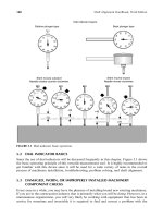
For example, Figure 8.6 shows a bracket attached to the shaft on the left holding a dial
indicator that is measuring the shaft on the right. When the bracket and indicator are rotated
to the bottom, the stem of the dial indicator was pushed in as it traversed from the top to the
bottom of the shaft on the right. When indicator stems set is pushed in, the needle sweeps in a
clockwise direction, producing a positive number. Therefore the shaft on the right is ‘‘low’’
with respect to the shaft on the left.
The body of the dial
indicator stays at the
same distance from the
centerline of rotation of
the shaft it is attached to.
FIGURE 8.6 Positive reading indicates that the shaft you are measuring is ‘‘low.’’ The stem of the dial
indicator was pushed in as it traversed from the top to the bottom of the shaft on the right. When
indicator stems set is pushed in, the needle sweeps in a clockwise direction producing a positive number.
Therefore the shaft on the right is ‘‘low’’ with respect to the shaft on the left.
Piotrowski / Shaft Alignment Handbook, Third Edition DK4322_C008 Final Proof page 326 6.10.2006 12:13am

326 Shaft Alignment Handbook, Third Edition
Figure 8.7 shows a bracket attached to the shaft on the left holding a dial indicator that is
measuring the shaft on the right. When the bracket and indicator are rotated to the bottom,
the stem of the dial indicator traveled outward as it traversed from the top to the bottom of
the shaft on the right. When indicator stems travel outward, the needle sweeps in a counter-
clockwise direction producing a negative number. Therefore the shaft on the right is ‘‘high’’
with respect to the shaft on the left.
The quotation marks around the words ‘‘low’’ and ‘‘high’’ are there for a reason. ‘‘High’’
and ‘‘low’’ are relative terms and only apply if you are viewing horizontally mounted shafts
when looking at them in the side view (up and down direction). If for example, you are
looking at the shafts in Figure 8.6 from above and the top of the page is north, the shaft on
the right in Figure 8.6 would appear to be to the south of the shaft on the right (positive (þ)
indicator reading). Likewise if you are looking at the shafts in Figure 8.7 from above and the
top of the page is north, the shaft on the right in Figure 8.7 would appear to be to the north of
the shaft on the right (negative (À) indicator reading).
This sounds very simple but in fact more people have trouble plotting shafts in the top view.
Again, it is important to understand what happens to the stem of the indicator as you traverse
from one side of a shaft to the other side. Does the stem get pushed in (i.e., go positive) or
does it have to travel outward (i.e., go negative)?
8.4.4 ZERO THE INDICATOR ON THE SIDE THAT IS POINTING TOWARD THE TOP
OF THE
GRAPH PAPER
In a horizontally mounted drive system, when you are viewing the alignment model in the side
view, you will only need to plot the dial indicator measurements you got on the top of the
shaft and on the bottom of the shaft. The readings you got on each side (north and south or
east and west or left and right) only come into play in the top view.
Classically when people initially set up their alignment measurement system the dial
indicator is placed on the top of a shaft in the twelve o’clock position, zero the indicator
The body of the dial
indicator stays at the

same distance from the
centerline of rotation of
the shaft it is attached to.
FIGURE 8.7 Negative reading indicates that the shaft you are measuring is ‘‘high.’’ The stem of the dial
indicator traveled outward as it traversed from the top to the bottom of the shaft on the right. When
indicator stems travel outward, the needle sweeps in a counterclockwise direction producing a negative
number. Therefore the shaft on the right is ‘‘high’’ with respect to the shaft on the left.
Piotrowski / Shaft Alignment Handbook, Third Edition DK4322_C008 Final Proof page 327 6.10.2006 12:13am
Alignment Modeling Basics 327
there and sweep through 908 arcs for the other three measurements as shown in Figure 6.35
through Figure 6.38.
8.4.5 WHATEVER SHAFT THE DIAL INDICATOR IS TAKING READINGS ON IS THE SHAFT THAT YOU
WANT TO DRAW ON THE GRAPH PAPER
Again, when viewing the alignment model in the side view you want to plot the measurements
you got from the top to the bottom of the shaft. Since you typically zero the indicator on the top
and sweep to the bottom, you will plot half of the bottom rim reading onto the alignment
model. A line representing the centerline of rotation of the pump shaft is drawn from the
position where the bracket was attached to the motor shaft through the point where the dial
indicator measured the position of the pump shaft as shown in Figure 8.8. Note the scale factor
in the lower left corner of the alignment model. Remember, you only plot half of the bottom
reading onto the graph. Also remember that whatever shaft the dial indicator is taking readings
on is the shaft that you want to draw on the graph paper. In this case, it is the pump shaft.
Motor Pump
Side view
Scale:
20 mils
5 in.
10 mils
Pump
Up

Motor
Sag
compensated
readings
Plot half (10 mils) of
this measurement
here.
T
B
W
−10+30
+20
0
Pump
E
FIGURE 8.8 (See color insert following page 322.) Plotting the pump shaft in the side view.
Piotrowski / Shaft Alignment Handbook, Third Edition DK4322_C008 Final Proof page 328 6.10.2006 12:13am
328 Shaft Alignment Handbook, Third Edition
A line representing the centerline of rotation of the motor shaft is drawn from the position
where the bracket was attached to the pump shaft through the point where the dial indicator
measured the position of the motor shaft as shown in Figure 8.9. Remember, you only plot
half of the bottom reading onto the graph. Also remember that whatever shaft the dial
indicator is taking readings on is the shaft that you want to draw on the graph paper. In
this case, it is the motor shaft.
Figure 8.9 now shows an exaggerated picture of the misalignment condition of the motor and
pump shafts in the up and down direction. But where are the shafts in the side-to-side direction?
When viewing the alignment model in the top view you want to plot the measurements you
got from one side of the shaft to the other side of the shaft and here is where a lot of mistakes
are classically made. Since you did not zero the indicator on one of the sides, how do you
handle the side readings? Real simple, zero the indicator on the side that is pointing toward

the top of the graph paper.
Motor Pump
Side view
Scale:
20 mils
Motor
Plot half (20 mils) of
this measurement
here.
Sag
compensated
readings
0
T
B
WE
−40
+10−50
5 in.
20
mils
Motor Pump
Up
FIGURE 8.9 (See color insert following page 322.) Plotting the motor shaft in the side view.
Piotrowski / Shaft Alignment Handbook, Third Edition DK4322_C008 Final Proof page 329 6.10.2006 12:13am
Alignment Modeling Basics 329
You have to imagine that you are now looking at your drive system from above. When you
are looking at the drive system from the side view with the motor to your left and the pump to
your right, which way are you looking (north, south, east, or west)? Getting this direction
correct is very important because there is nothing worse than moving your machinery the

right amount in the wrong direction.
In our motor and pump drive system we are working on here, let us say that we are looking
toward the east as we view the machinery as shown in Figure 8.8 and Figure 8.9. Now that
we are going to be viewing our machines from above when modeling the top view, we want
to zero the indicator on the side that is pointing toward the top of the graph paper and plot
the reading that is on the side that is pointing toward the bottom of the graph paper. In this
case, the direction pointing toward the top of the graph paper in the top view is going to be
east. Therefore we want to zero the indicator on the east side of each shaft and plot the
reading we will obtain on the west side of each shaft.
There are two ways that we can do this. One way is to physically rotate the bracket and
indicator over to the east side of each shaft, zero the indicator there, and then rotate the bracket
and dial indicator 1808 over to the west side and record the dial indicator readings we get there.
The other way is to mathematically manipulate the east and west reading we obtained from the
complete set of dial indicator readings to zero the east sides. Figure 8.10 shows how to perform
this math on the east and west readings.
Original sag compensated readings
Motor
0
0
+30
−10
+20
−40
0+50 = +50
−50+50 = 0
+10+50 = +60
−40+50 = +10
0–30 = –30
+30−30 = 0
−10−30 = −40

+20−30 = −10
T
T
EW
B
E
T
T
EW
B
EW
B
T
T
E
W
B
E
E
E
W
W
W
B
W
B
+10−50
Pump
Motor
Motor

Motor
Pump
Pump
Pump
Sag
compensated
readings
Sag
compensated
readings
Sag
compensated
readings
Mathematcially zero the east readings
Original sag compensated readings with the east reading zeroed
−10
0
0
+60
−40
0
+60
−50
+10
0 −40
+30
East to west readings to be plotted in the top view
FIGURE 8.10 Zeroing the east readings.
Piotrowski / Shaft Alignment Handbook, Third Edition DK4322_C008 Final Proof page 330 6.10.2006 12:13am
330 Shaft Alignment Handbook, Third Edition

The original readings with the indicator zeroed on the top and the new readings with the
indicator zeroed on the east are telling us the same thing about the misalignment condition
between the two shafts. All we did was zero the indicator in a different position and notice
that the validity rule still applies whether we zero on top or on the east. Now that we are going
to be plotting the shafts in the top view, the top and bottom readings are meaningless, only
the east and west readings are important.
Figure 8.11 and Figure 8.12 show how to plot the east and west readings onto the top view
alignment model. Notice that the scale factor in the top view is not the same as the scale factor
in the side view. They do not have to be the same scale factor in both views but remember
what the scale factors are in each view. Without being too repetitive here, remember that you
only plot half of the dial indicator reading onto the graph. Also remember that whatever shaft
the dial indicator is taking readings on is the shaft that you want to draw on the graph paper.
Two of the major graphing mistakes people make are to forget to only plot half of the rim
reading and drawing the wrong shaft onto the graph.
The alignment models shown in Figure 8.9 through Figure 8.12 were generated using the
reverse indicator method, which is covered in more detail in Chapter 10. The other four alignment
Motor
Motor
Top view
East
Pump
Pump
20 mils
Scale:
5 in.
540 mils
Notice the scale
factor here.
Plot half (20 mils)
of this

measurement here.
0
E
W
−40
Pump
FIGURE 8.11 (See color insert following page 322.) Plotting the pump shaft in the top view.
Piotrowski / Shaft Alignment Handbook, Third Edition DK4322_C008 Final Proof page 331 6.10.2006 12:13am
Alignment Modeling Basics 331
methods (face–rim, double radial, shaft to coupling spool, and face–face) and their associated
graphing and modeling techniques will be discussed in Chapter 11 through Chapter 15.
8.4.6 DETERMINING CORRECTIVE MOVES TO MAKE ON ONE MACHINE FROM
THE
ALIGNMENT MODEL
Let us look at another example. Figure 8.13 shows a motor and a fan shaft misalignment
condition in the side view. As you can see, the shafts are not in alignment with each other.
Now what do we do? The next logical step is to determine the movement restrictions imposed
on the machine cases at the control or adjustment points (i.e., where the foot bolts are).
Movement restrictions define the boundary condition that help you to make an intelligent
decision on what alignment correction would be easy and trouble free to accomplish.
Trouble-free movement solutions? I fully understand that any corrective moves you make
on rotating machinery are not going to be trouble free and easy to make. But there are some
moves that will be far more difficult to make than others. You really need to have a wide
Motor
Motor
Pump
Pump
Top view
East
Plot half (30 mils)

of this
measurement here.
Motor
0
E
W
+60
Scale:
5 in.
20 mils
30 mils
FIGURE 8.12 (See color insert following page 322.) Plotting the motor shaft in the top view.
Piotrowski / Shaft Alignment Handbook, Third Edition DK4322_C008 Final Proof page 332 6.10.2006 12:13am
332 Shaft Alignment Handbook, Third Edition
variety of options to make the most effective and intelligent alignment correction. Therefore,
keep an open, objective mindset when you attempt to fix your alignment problem.
In Figure 8.13, notice that if you wanted to keep the fan in its current position, you would
have to move the motor downward at both the inboard and outboard ends. As shown in
Figure 8.13, the amount of movement at the outboard bolts is obtained by counting the
number of squares (at 3 mils per square with this scale factor) from where the actual motor
shaft centerline is at the outboard bolting plane to the extended centerline of rotation of the
fan. In this particular case, this is, 166 mils (0.166 in.). The amount of movement at the
inboard bolts is obtained by counting the number of squares from where the actual motor
shaft centerline is at the inboard bolting plane to the extended centerline of rotation of the
fan. In this case, that is, 66 mils (0.066 in.). If there is 166 mils under both outboard bolts and
66 mils under both inboard bolts (that are not soft foot shims) then a good alignment solution
would be to remove that amount of shim stock from under the appropriate feet. But what if
there are not that many shims under the inboard and outboard feet?
As bizarre as this may sound, I have seen people in a situation like this, remove the motor
from the baseplate and grind the baseplate away. Unbelievable, but true. And it is still done

somewhere today.
8.4.7 OVERLAY LINE OR FINAL DESIRED ALIGNMENT LINE
The final desired alignment line (a.k.a. the overlay line) is a straight line drawn on top of the
graph, showing the desired position both shafts should be in to achieve colinearity of
centerlines. It should be apparent that if one machine case is stationary, in this case the fan
shaft, that machine’s centerline of rotation is the final desired alignment line as shown in
Figure 8.13.
There is another way to correct the misalignment problem on this motor and fan that will
be far less troublesome. Since adjustments are made at the inboard and outboard feet of the
machinery, some logical alternative solutions would be to consider using one or more of these
feet as pivot points. Both outboard feet or both inboard feet, or the outboard foot of one
machine case and the inboard foot of the other machine case could be used as pivot points. By
Up
Motor
Side view
Fan
Motor shaft centerline
66 mils down
166 mils down
Scale:
5 in.
30 mils
Fan shaft
centerline
FIGURE 8.13 Movement solutions for the motor only.
Piotrowski / Shaft Alignment Handbook, Third Edition DK4322_C008 Final Proof page 333 6.10.2006 12:13am
Alignment Modeling Basics 333
drawing the overlay line through these foot points, shaft alignment can usually be achieved
with smaller moves. In real life situations, you will typically have greater success aligning two
machine cases a little bit rather than moving one machine case a lot. Figure 8.14 shows using

the overlay line to connect the outboard bolting plane of the motor with the outboard bolting
plane of the fan. The inboard bolting planes are then moved the amount shown in Figure 8.14
to correct the misalignment condition in the up and down direction. No shims had to be
removed and better yet, no baseplates had to be ground away.
8.4.8 SUPERIMPOSE YOUR BOUNDARY CONDITIONS,MOVEMENT RESTRICTIONS, AND
ALLOWABLE MOVEMENT ENVELOPE
When viewing the machinery in the up and down direction (side view), the movement
restrictions are defined by the amount of movement the machinery can be adjusted in the
up and down directions.
How far can machinery casings be moved upward? There is virtually an unlimited amount
of movement in the up direction, within reason, that is. Machine cases are typically moved
upward by installing shims (i.e., sheet metal of various thicknesses) between the undersides of
the machinery feet and the baseplate.
How far can the machinery casings be moved downward? Well, it depends on the amount
of shim stock currently under the machinery feet that are not soft foot corrections.
How far can you move a machine down? I don’t know. You are going to have to look
under the machine to see how much shim stock could be removed from under the machinery
feet on every machine in the drive system. Maybe there are 10, 20, or 50 mils of shim stock
under the machinery feet that can be removed that are not soft foot corrections that could be
taken out. You will have to see what is there. These shims define the ‘‘downward movement
envelope,’’ or as some people call it, the ‘‘basement floor,’’ or as other people call it, the
‘‘baseplate restriction point.’’
Shim stock typically refers to sheet metal thicknesses ranging from 1 mils (0.001 in.) to 125
mils (0.125 in.). There are several companies that manufacture precut, U-shaped shim stock in
Up
Side view
Raise 48 mils up
Overlay line
Motor
Pivot here

Motor shaft
centerline
Scale:
5 in.
30 mils
Raise 138 mils up
Fan
Pivot here
Fan shaft
centerline
FIGURE 8.14 (See color insert following page 322.) Movement solutions for the inboard feet of both the
motor and the pump by pivoting at the outboard feet of both machines.
Piotrowski / Shaft Alignment Handbook, Third Edition DK4322_C008 Final Proof page 334 6.10.2006 12:13am
334 Shaft Alignment Handbook, Third Edition
4 standard sizes and 17 standard thicknesses. Once shim thicknesses get over 125 mils, they
are typically referred to as spacers or plates and are custom made from plate steel.
So if you want to move a machine downward and there are no shims under the machinery
feet, you are already on the basement floor and that is defined as a downward vertical
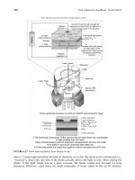
movement restriction or a baseplate restriction point. Figure 8.15 shows the same motor
and fan but now we have observed that there are 75 mils of shim stock under the outboard
feet and 25 mils of shims under the inboard feet that are not soft foot corrections that could be
removed if we wanted to. By counting down 75 mils from the centerline of the motor shaft
and the outboard bolting plane and drawing a baseplate restriction point there, we can now
see how far that end can come down without removing metal from the baseplate or machine
casing. Similarly, by counting down 25 mils from the centerline of the motor shaft and the
inboard bolting plane and drawing a baseplate restriction point there, we can now see how far
that end can come down without removing metal. In this particular case, there were no shims
under any of the feet of the fan so its baseplate restriction points are positioned directly on the
fan centerline at the inboard and outboard ends as shown in Figure 8.15. Now that we know
what the lowest points of downward movement could be without removing metal, one

possible solution would be to use the outboard feet of the fan and the inboard feet of the
motor as pivot points removing 72 mils of shims from under the outboard feet of the motor
and installing 42 mils of shims under the inboard feet of the fan as shown in Figure 8.15.
8.4.8.1 Lateral Movement Restrictions
In addition to aligning machinery in the up and down direction, it is also imperative that the
machinery be aligned properly side to side. Machinery is aligned side to side by translating the
machine case laterally. This sideways movement is typically monitored by setting up dial
indicators along the side of the machine case at the inboard and outboard hold down bolts,
anchoring the indicators to the frame or baseplate, zeroing the indicators, and then moving
the inboard and outboard ends the prescribed amounts. Here is where realignment typically
becomes extremely frustrating since there is a limited amount of room between the shanks of
the hold down bolts and the holes drilled in the machine case feet.
Up
Side view
Overlay line
Motor
Pivot here
Lower 72 mils
down
75 mils of
shims
available to
remove
25 mils of
shims
available to
remove
Scale:
5 in.
30 mils

Baseplate restriction points
Raise 42 mils up
Fan
pivot here
No shims
available to
remove
Fan shaft
centerline
No shims
available to
remove
FIGURE 8.15 (See color insert following page 322.) Movement solutions using the outboard feet of the
fan and the inboard feet of the motor as pivot points.
Piotrowski / Shaft Alignment Handbook, Third Edition DK4322_C008 Final Proof page 335 6.10.2006 12:13am
Alignment Modeling Basics 335
If, for example, you wanted to move the outboard end of a machine 120 mils to the south,
began moving the outboard end monitoring the move with a dial indicator, and the machine
case stopped moving after 50 mils of translation, this would be considered a movement
restriction commonly referred to as a ‘‘bolt bound’’ condition. The problem in moving
machinery laterally is that there is a limited amount of allowable movement in either
direction. The total amount of side-to-side movement at each end of the machine case is
referred to as the ‘‘lateral movement envelope.’’ To find the allowable lateral movement
envelope, remove a bolt from each end of the machine case, look down the hole, and see how
much room exists between the shank of the bolt and the hole drilled in the machine case at
that foot. If necessary, thread the bolt into the hole a couple of turns, and measure the gaps
between the bolt shank and the sides of the hole with feeler or wire gauges.
It is very important for one to recognize that trouble free alignment corrections can only be
achieved when the allowable movement envelope is known. Perhaps one of the most import-
ant statements that will be made in this chapter is

When you consider that both machine cases are movable, there are an infinite number of possible
ways to align the shafts, some of which fall within the allowable movement envelope.
It seems ridiculous, but many people have ground baseplates or the undersides of machin-
ery feet away because they felt that a machine had to be lowered. When machinery becomes
bolt bound when trying to move it sideways, people frequently cut down the shanks of the
bolts or grind a hole open more.
There is typically an easier solution. Disappointingly, many of the alignment measurement
systems shown in this book force the user to name one machine case stationary and the other one
movable which will invariably cause repositioning problems when the machine case has to be
moved outside its allowable movement envelope. This may not happen the first time you align a
drive system, or the second or third time, but if you align enough machinery, eventually you will
not be able to move the movable machine the amount prescribed. Once the centerlines of rotation
have been determined and the allowable movement envelope illustrated on the graph, it becomes
very apparent what repositioning moves will work easily and which ones will not.
Figure 8.16 shows the top view alignment model of a motor and pump. Not knowing any
better, it appears that all you would have to do is move the outboard end of the motor 14 mils
to the east and the inboard end of the motor 4 mils to the west. Easy enough. But what if the
outboard end of the motor is bolt bound to the east already?
By removing one bolt from the inboard and outboard ends of both the motor and pump,
the lateral movement restrictions can be observed. In this case the following restrictions were
observed:
1. Outboard end of motor—bolt bound to east and 40 mils of possible movement to the
west
2. Inboard end of motor—bolt bound to east and 40 mils of possible movement to the west
3. Inboard end of pump—32 mils of possible movement to the east and 8 mils of possible
movement to the west
4. Outboard end of pump—36 mils of possible movement to the east and 4 mils of possible
movement to the west
By plotting the eastbound and westbound restriction onto the alignment model, you can
now see the easy corridor of movement. One possible solution (out of many) is shown in

Figure 8.16.
Piotrowski / Shaft Alignment Handbook, Third Edition DK4322_C008 Final Proof page 336 6.10.2006 12:13am
336 Shaft Alignment Handbook, Third Edition
Please, for your own sake, follow these four basic steps to prevent you from wasting hours
or days of your time correcting a misalignment condition:
1. Find the positions of every shaft in the drive train by the graphing and modeling
techniques shown in this and later chapters.
2. Determine the total allowable movement envelope of all the machine cases in both
directions.
3. Plot the restrictions on the graph or model.
4. Select a final desired alignment line or overlay line that fits within the allowable
movement envelope (hopefully) and move the machinery to that line.
If you are involved with aligning machinery, by following the four steps above, it is
guaranteed that you will save countless hours of wasted time trying to move one machine
where it does not really want to go.
8.4.8.2 Where Did the Stationary–Movable Alignment Concept Come From?
I don’t know. Every piece of rotating machinery in existence has, at one time or another, been
placed there. Mother Earth never gave birth to a machine. They are neither part of the Earth’s
mantle nor firmly imbedded in bedrock. Every machine is movable, it is just a matter of effort
(pain) to reposition it. So why have the vast majority of people who align machinery called
one machine stationary and the other machine movable?
The only viable reason that I can come up with is this—in virtually every industry there is
an electric motor driving a pump. When you first approach a motor pump arrangement, you
immediately notice that the pump has piping attached to it and the only appendage attached
to the motor is conduit (usually flexible conduit). From your limited vantage point at this
time it would appear to be easier to move the motor because there is no piping attached to it
like the pump. You would prefer to just move the motor because it looks easier to move than
the pump (and so would I). The assumption is made that the pump will not be moved, no
matter what position you find the motor shaft in with respect to the pump shaft.
Motor

Top view
32 mils of
possible
movements to
the east here
Pivot here
Pump
36 mils of
possible
movement to
the east here
Move 14 mils
east here
4 mils of
possible
movement
to the west
here
8 mils of
possible
movement
to the west
here
Lateral movement restriction points
40 mils of
possible
movement
to the west here
20 mils
5 in.

Scale:
Move 20 mils
west here
East boundary line
West boundary line
Move 22 mils
west here
Bolt bound
to east
here
East
FIGURE 8.16 (See color insert following page 322.) Applying lateral movement restrictions to arrive at
an easy sideways move within the east and west corridors.
Piotrowski / Shaft Alignment Handbook, Third Edition DK4322_C008 Final Proof page 337 6.10.2006 12:13am
Alignment Modeling Basics 337
But what do you do when you have to align a steam turbine driving a pump? They are both
piped; which machine do you call the stationary machine—the pump or the turbine? No
matter what your answer is, you are going to have to move one of them and they both have
piping attached to their casings.
Piping is no excuse not to move a piece of machinery, particularly in light of what most of
us know about how piping is really attached to machinery. For some people, they are afraid
to loosen the bolts holding a machinery with piping attached to it because the piping strain is
so severe that they fear the machine will shift so far that it will never get back into alignment.
So is the problem with the alignment process or the piping fit-up? Refer to Chapter 3 for
information on this subject.
If you align enough machinery and insist that one machine will be stationary, eventually
you will get exactly what you deserve for your shallow range of thinking.
8.4.8.3 Solving Piping Fit-Up Problems with the Overlay Line
Although we have been showing that the overlay line (a.k.a. final desired alignment line) is
drawn through foot bolt points, it is important to see that the overlay line could be drawn

anywhere and the machinery shafts moved to that line.
This can be particularly beneficial if there are other considerations that have to be taken
into account such as piping fit-up problems. Figure 8.17 shows a motor and pump where the
suction pipe is 1=4 in. higher than the suction flange on the pump and there is a 1=4 in.
excessive gap at the discharge flanges. Rather than align both shafts, then install an additional
0.250Љ
Motor
Pump
15Љ
Motor Pump
Side view
15Љ 5.5Љ
Bracket clamping positions
Scale:
Suction flange location
7Љ 14.5Љ10Љ
5.5Љ 7Љ 14.5Љ 5Љ
10.25Љ
1Љ 1Љ
0.250Љ
5 in.
FIGURE 8.17 (See color insert following page 322.) Scaling off the dimensions for a motor and pump
including the location of the suction flange on the pump.
Piotrowski / Shaft Alignment Handbook, Third Edition DK4322_C008 Final Proof page 338 6.10.2006 12:13am
338 Shaft Alignment Handbook, Third Edition
250 mils (1=4 in.) under all the feet, another easier solution exists. Scale off where the suction
flange of the pump is onto the alignment model. Extend the centerline of the pump to go out
to the suction flange point. Place a mark 250 mils above the pump shaft centerline where the
suction flange is located. Construct an overlay line to go from that point to the outboard bolts
of the motor as illustrated in Figure 8.18. Then solve for the moves at each bolting plane not

only to eliminate the piping fit-up problem but also to align the shafts.
We have reviewed many of the basic concepts behind alignment modeling in this chapter.
Determining your maximum misalignment deviation and whether you are within acceptable
alignment tolerances will be covered in the next chapter. Specific instruction on how to
perform all five-alignment measurement methods and their associated modeling techniques
will be covered in Chapter 10 through Chapter 15.
BIBLIOGRAPHY
Dodd, V.R., Total Alignment, Petroleum Publishing Company, Tulsa, OK, 1975.
Dreymala, J., Factors Affecting and Procedures of Shaft Alignment, Technical and Vocational Depart-
ment, Lee College, Baytown, TX, 1970.
Piotrowski, J., Basic Shaft Alignment Workbook, Turvac Inc., Cincinnati, OH, 1991.
Suction flange moves up
250 mils at this point
Pivot here
Raise 47 mils up
Scale:
5 mils
Motor
0
T
B
E
W
T
B
E
W
−60
+10 +90
+80

0
−
10
Sag
compensated
readin
g
s
−70
Pump
Up
Side view
Raise 170 mils up
Raise 235 mils up
5 in.
FIGURE 8.18 (See color insert following page 322.) Overlay line positioned to correct the piping fit-up
problem and align the shafts with one move.
Piotrowski / Shaft Alignment Handbook, Third Edition DK4322_C008 Final Proof page 339 6.10.2006 12:13am
Alignment Modeling Basics 339
Piotrowski / Shaft Alignment Handbook, Third Edition DK4322_C008 Final Proof page 340 6.10.2006 12:13am
9
Defining Misalignment:
Alignment and Coupling
Tolerances
9.1 WHAT EXACTLY IS SHAFT ALIGNMENT?
In very broad terms, shaft misalignment occurs when the centerlines of rotation of two (or
more) machinery shafts are not in line with each other. Therefore, in its purest definition,
shaft alignment occurs when the centerlines of rotation of two (or more) shafts are collinear
when operating at normal conditions. As simple as that may sound, there still exists a
considerable amount of confusion to people who are just beginning to study this subject

when trying to precisely define the amount of misalignment that may exist between two shafts
flexibly or rigidly coupled together.
How do you measure misalignment when there are so many different coupling designs?
Where should the misalignment be measured? Is it measured in terms of mils, degrees,
millimeters of offset, arcseconds, radians? How accurate does the alignment have to be?
When should the alignment be measured, when the machines are off-line or when they are
running? Perhaps a commonly asked question needs to be addressed first.
9.2 DOES LEVEL AND ALIGNED MEAN THE SAME THING?
The level and aligned does not mean the same thing. The term ‘‘level’’ is related to Earth’s
gravitational pull. When an object is in a horizontal state or condition or points along the
length of the centerline of an object are at the same altitude, the object is considered to be
level. Another way of stating this is that an object is level if the surface of the object is
perpendicular to the lines of gravitational force. A level rotating machinery foundation
located in Boston would not be parallel to a level rotating machinery foundation located in
San Francisco as the Earth’s surface is curved. The average diameter of the Earth is 7908.5
miles (7922 miles at the equator and 7895 miles at the poles due to the centrifugal force
causing the planet to bulge at the center). When measuring the distances of arc across the
Earth’s surface, 18 of arc is slightly over 69 miles, 1 min of arc is slightly over 1.15 miles, and
one second of arc is slightly over 101.2 ft.
It is possible, although rare, to have a machinery drive train both level and aligned. It is
also possible to have a machinery drive train level but not aligned and it is also possible to
have a machinery drive train aligned but not level. As shaft alignment deals specifically with
the centerlines of rotation of machinery shafts it is possible to have, or not to have, the
centerlines of rotation perpendicular to the lines of gravitational force.
Historically, there were a considerable number of patents filed from 1900 to 1950 that
seemed to combine (or maybe confuse) the concept of level and aligned. A number of these
Piotrowski / Shaft Alignment Handbook, Third Edition DK4322_C009 Final Proof page 341 26.9.2006 8:42pm
341
alignment devices were used in the paper industry where extremely long ‘‘line shafts’’ were
installed to drive different parts of a paper machine. These line shafts were constructed with

numerous sections of shafting that were connected end to end with rigid couplings and
supported by a number of bearing pedestals along the length of the drive system, which
could be 300 ft in length or more. Even if a mechanic carefully aligned each section of shafting
at each rigid coupling connection along the length of the line shaft and perfectly leveled each
shaft section, the centerline of rotation at each end of a 300-ft long line shaft would be out by
0.018 in. due to the curvature of the Earth’s surface.
Although level and aligned may not mean the same thing, proper leveling is important as well
as having coplanar surfaces. Levelness refers to a line or surface, which is perpendicular to
gravity; coplanar surface refers to ‘‘flatness.’’ Are the points where the machinery cases contact
the baseplate (or soleplates) in the same plane? If not, how much of a deviation is there?
It is very common to see baseplates where the machinery contact surfaces are not in the same
plane or several soleplates that contact a single machine case not be in the same plane. This
coplanar deviation may be a contributor to a condition commonly referred to as a ‘‘soft foot’’
problem and was covered in Chapter 5. Figure 9.1 shows the recommended guidelines for leveling
machinery baseplates and coplanar surface deviation. As will be seen, even if the surfaces of a
baseplate are perfectly level and perfectly coplanar, a soft foot condition could still exist.
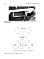
9.3 MEASURING ANGLES
Angular misalignment is shown in Figure 9.2. As the term ‘‘angular’’ or ‘‘angle’’ is used, it is
necessary to briefly describe how angles are measured.
There are 3608 in a circle. Each degree can be divided into 60 parts called minutes of arc and
each minute of arc can be further divided into 60 parts called seconds of arc. Therefore there
are 21,600 min of arc and 1,296,000 s of arc in a circle.
General process
machinery supported
in antifriction bearings
10 mils per foot 10 mils
General process
machinery supported
in sleeve bearings
(up to 500 hp)

5 mils per foot
Process machinery
supported in
antifriction bearings
(500+ hp)
5 mils per foot
Process machinery
supported in sleeve
bearings (500+ hp)
2 mils per foot
Machine tools
1 mil per foot
Note: 1 mil = 0.001 in.
5 mils
5 mils
5 mils
2 mils
Machinery Type
Minimum
Recommended
Levelness
Coplanar
Surface
Deviation
FIGURE 9.1 Recommended levelness and coplanar surface deviation for rotating machinery baseplates
or soleplates.
Piotrowski / Shaft Alignment Handbook, Third Edition DK4322_C009 Final Proof page 342 26.9.2006 8:42pm
342 Shaft Alignment Handbook, Third Edition
Another way of expressing circles is by use of radians. All circles are mathematically related
by an irrational number called pi (p), which is approximately equal to 3.14159. There are 2p

radians in a circle. Therefore one radian is equal to 57.2958288.
Despite the fact that the expression ‘‘angular misalignment’’ is used frequently it comes as a
surprise to learn that no known shaft alignment measurement system actually uses an angular
measurement sensor or device.
9.4 TYPES OF MISALIGNMENT
Shaft misalignment can occur in two basic ways: parallel and angular as shown in Figure 9.2.
Actual field conditions usually have a combination of both parallel and angular misalignment
so measuring the relationship of the shafts gets to be a little complicated in a three-
dimensional world especially when you try to show this relationship on a two-dimensional
piece of paper. I find it helpful at times to take a pencil in each hand and position them based
on the dial indicator readings to reflect how the shafts of each unit are sitting.
9.5 DEFINITION OF SHAFT MISALIGNMENT
In more precise terms, shaft misalignment is the deviation of relative shaft position from a
collinear axis of rotation measured at the flexing points in the coupling when equipment is
running at normal operating conditions. To better understand this definition, let us dissect
each part of this statement to clearly illustrate what is involved.
Parallel misalignment
Angular misalignment
“Real world” misalignment usually
exhibits a combination of both
parallel and angular conditions
FIGURE 9.2 How shafts can be misaligned.
Piotrowski / Shaft Alignment Handbook, Third Edition DK4322_C009 Final Proof page 343 26.9.2006 8:42pm
Defining Misalignment: Alignment and Coupling Tolerances 343
Collinear means in the same line or in the same axis. If two shafts are collinear, then they
are aligned. The deviation of relative shaft position accounts for the measured difference
between the actual centerline of rotation of one shaft and the projected centerline of rotation
of the other shaft.
There are literally dozens of different types of couplings. Rather than have guidelines for
each individual coupling, it is important to understand that there is one common design

parameter that applies to all flexible couplings:
For a flexible coupling to accept both parallel and angular misalignment there must be at least two
points along the projected shaft axes where the coupling can flex or articulate to accommodate the
misalignment condition.
The rotational power from one shaft is transferred over to another shaft through these
flexing points. These flexing points are also referred to as flexing planes or points of power
transmission. Shaft alignment accuracy should be independent of the type of coupling used
and should be expressed as a function of the shaft positions, not the coupling design or the
mechanical flexing limits of the coupling. Figure 9.3 illustrates where the flexing points in a
variety of different coupling designs are located. I have seen several instances where there is
only one flexing point in the coupling and have also seen more than two flexing points in the
coupling connecting two shafts together. If only one flexing point is present and there is an
offset between the shafts or a combination of an angle and an offset, there will be some very
high radial forces transmitted across the coupling into the bearings of the two machines. If
there are more than two flexing points, there will be a considerable amount of uncontrolled
motion in between the two connected shafts, usually resulting in very high vibration levels in
the machinery.
Why should misalignment be measured at the flexing points in the coupling? Simply
because that is where the coupling is forced to accommodate the misalignment condition
and that is where the action, wear, and power transfer across the coupling is occurring.
Flex points
Flex points
Flex points
Flex points
Flex points
Flex points
FIGURE 9.3 Flexing point locations in a variety of couplings.
Piotrowski / Shaft Alignment Handbook, Third Edition DK4322_C009 Final Proof page 344 26.9.2006 8:42pm
344 Shaft Alignment Handbook, Third Edition