Harris'''' Shock and Vibration Handbook Part 13 docx
Bạn đang xem bản rút gọn của tài liệu. Xem và tải ngay bản đầy đủ của tài liệu tại đây (918.09 KB, 82 trang )
INFLUENCE OF DAMPING IN VIBRATION ISOLATION
The nature and degree of vibration isolation afforded by an isolator is influenced
markedly by the characteristics of the damper. This aspect of vibration isolation is
evaluated in this section in terms of the single degree-of-freedom concept; i.e., the
equipment and the foundation are assumed rigid and the isolator is assumed mass-
less. The performance is defined in terms of absolute transmissibility, relative trans-
missibility, and motion response for isolators with each of the four types of dampers
illustrated in Table 30.1. A system with a rigidly connected viscous damper is dis-
cussed in detail in Chap. 2, and important results are reproduced here for com-
pleteness; isolators with other types of dampers are discussed in detail here.
The characteristics of the dampers and the performance of the isolators are
defined in terms of the parameters shown on the schematic diagrams in Table 30.1.
Absolute transmissibility, relative transmissibility, and motion response are defined
analytically in Table 30.2 and graphically in the figures referenced in Table 30.2. For
the rigidly connected viscous and Coulomb-damped isolators, the graphs generally
are explicit and complete. For isolators with elastically connected dampers, typical
results are included and references are given to more complete compilations of
dynamic characteristics.
THEORY OF VIBRATION ISOLATION 30.5
TABLE 30.2 Transmissibility and Motion Response for
Isolation Systems Defined in Table 30.1 (Continued)
Where the equation is shown graphically, the applicable figure is indicated below the equa-
tion. See Table 30.1 for definition of terms.
NOTE 4: These curves apply only for N = 3.
N
OTE 5: This equation applies only when excitation is defined in terms of displacement amplitude; for
excitation defined in terms of force or acceleration, see Eq. (30.18).
8434_Harris_30_b.qxd 09/20/2001 11:41 AM Page 30.5
RIGIDLY CONNECTED VISCOUS DAMPER
Absolute and relative transmissibility curves are shown graphically in Figs. 30.2 and
30.3, respectively.* As the damping increases, the transmissibility at resonance
decreases and the absolute transmissibility at the higher values of the forcing fre-
quency ω increases; i.e., reduction of vibration is not as great. For an undamped iso-
lator, the absolute transmissibility at higher values of the forcing frequency varies
inversely as the square of the forcing frequency.When the isolator embodies signifi-
cant viscous damping, the absolute transmissibility curve becomes asymptotic at
high values of forcing frequency to a line whose slope is inversely proportional to
the first power of the forcing frequency.
The maximum value of absolute transmissibility associated with the resonant
condition is a function solely of the damping in the system, taken with reference to
critical damping. For a lightly damped system, i.e., for ζ<0.1, the maximum absolute
transmissibility [see Eq. (2.41)] of the system is
1
30.6 CHAPTER THIRTY
* For linear systems, the absolute transmissibility T
A
= x
0
/u
0
in the motion-excited system equals F
T
/F
0
in
the force-excited system. The relative transmissibility T
R
=δ
0
/u
0
applies only to the motion-excited system.
FIGURE 30.2 Absolute transmissibility for the
rigidly connected, viscous-damped isolation sys-
tem shown at A in Table 30.1 as a function of the
frequency ratio ω/ω
0
and the fraction of critical
damping ζ. The absolute transmissibility is the
ratio (x
0
/u
0
) for foundation motion excitation
(Fig. 30.1A) and the ratio (F
T
/F
0
) for equipment
force excitation (Fig. 30.1B).
FIGURE 30.3 Relative transmissibility for the
rigidly connected, viscous-damped isolation sys-
tem shown at A in Table 30.1 as a function of the
frequency ratio ω/ω
0
and the fraction of critical
damping ζ.The relative transmissibility describes
the motion between the equipment and the
foundation (i.e., the deflection of the isolator).
8434_Harris_30_b.qxd 09/20/2001 11:41 AM Page 30.6
T
max
= (30.1)
where ζ=c/c
c
is the fraction of critical damping defined in Table 30.1.
The motion response is shown graphically in Fig. 30.4. A high degree of damping
limits the vibration amplitude of the equipment at all frequencies, compared to an
undamped system.The single degree-of-freedom system with viscous damping is dis-
cussed more fully in Chap. 2.
RIGIDLY CONNECTED COULOMB DAMPER
The differential equation of motion for the system with Coulomb damping shown in
Table 30.1B is
m¨x + k(x − u) ± F
f
= F
0
sin ωt (30.2)
The discontinuity in the damping force that occurs as the sign of the velocity
changes at each half cycle requires a step-by-step solution of Eq. (30.2).
2
An
approximate solution based on the equivalence of energy dissipation involves
equating the energy dissipation per cycle for viscous-damped and Coulomb-
damped systems:
3
πcωδ
0
2
= 4F
f
δ
0
(30.3)
where the left side refers to the viscous-
damped system and the right side to the
Coulomb-damped system; δ
0
is the
amplitude of relative displacement
across the damper. Solving Eq. (30.3)
for c,
c
eq
==j
(30.4)
where c
eq
is the equivalent viscous damp-
ing coefficient for a Coulomb-damped
system having equivalent energy dissi-
pation. Since
˙
δ
0
= jωδ
0
is the relative
velocity, the equivalent linearized dry
friction damping force can be consid-
ered sinusoidal with an amplitude
j(4F
f
/π). Since c
c
= 2k/ω
0
[see Eq. (2.12)],
ζ
eq
== (30.5)
where ζ
eq
may be defined as the equiva-
lent fraction of critical damping. Substi-
tuting δ
0
from the relative transmissibility
expression [(b) in Table 30.2] in Eq.
(30.5) and solving for ζ
eq
2
,
2ω
0
F
f
ᎏ
πωkδ
0
c
eq
ᎏ
c
c
4F
f
ᎏ
π
˙
δ
0
4F
f
ᎏ
πωδ
0
1
ᎏ
2ζ
THEORY OF VIBRATION ISOLATION 30.7
FIGURE 30.4 Motion response for the
rigidly connected viscous-damped isolation sys-
tem shown at A in Table 30.1 as a function of
the frequency ratio ω/ω
0
and the fraction of
critical damping ζ. The curves give the resulting
motion of the equipment x in terms of the exci-
tation force F and the static stiffness of the iso-
lator k.
8434_Harris_30_b.qxd 09/20/2001 11:41 AM Page 30.7
ζ
eq
2
=
η
2
1 −
2
(30.6)
΄
−
η
2
΅
where η is the Coulomb damping parameter for displacement excitation defined in
Table 30.1.
The equivalent fraction of critical damping given by Eq. (30.6) is a function of the
displacement amplitude u
0
of the excitation since the Coulomb damping parameter
η depends on u
0
. When the excitation is defined in terms of the acceleration ampli-
tude ü
0
, the fraction of critical damping must be defined in corresponding terms.
Thus, it is convenient to employ separate analyses for displacement transmissibility
and acceleration transmissibility for an isolator with Coulomb damping.
Displacement Transmissibility. The absolute displacement transmissibility of an
isolation system having a rigidly connected Coulomb damper is obtained by substi-
tuting ζ
eq
from Eq. (30.6) for ζ in the absolute transmissibility expression for viscous
damping, (a) in Table 30.2. The absolute displacement transmissibility is shown
graphically in Fig. 30.5, and the relative displacement transmissibility is shown in Fig.
30.6. The absolute displacement transmissibility has a value of unity when the forc-
ing frequency is low and/or the Coulomb friction force is high. For these conditions,
the friction damper is locked in, i.e., it functions as a rigid connection, and there is no
relative motion across the isolator.The frequency at which the damper breaks loose,
4
ᎏ
π
ω
4
ᎏ
ω
0
4
ω
2
ᎏ
ω
0
2
ω
2
ᎏ
ω
0
2
2
ᎏ
π
30.8 CHAPTER THIRTY
FIGURE 30.5 Absolute displacement trans-
missibility for the rigidly connected, Coulomb-
damped isolation system shown at B in Table 30.1
as a function of the frequency ratio ω/ω
0
and the
displacement Coulomb-damping parameter η.
FIGURE 30.6 Relative displacement transmis-
sibility for the rigidly connected, Coulomb-
damped isolation system shown at B in Table 30.1
as a function of the frequency ratio ω/ω
0
and the
displacement Coulomb-damping parameter η.
8434_Harris_30_b.qxd 09/20/2001 11:41 AM Page 30.8
THEORY OF VIBRATION ISOLATION 30.9
* This equation is based upon energy considerations and is approximate. Actually, the friction damper
breaks loose when the inertia force of the mass equals the friction force, mu
0
ω
2
= F
f
.This gives the exact solu-
tion (ω/ω
0
)
L
=
͙
η
ෆ
. A numerical factor of 4/π relates the Coulomb damping parameters in the exact and
approximate solutions for the system.
i.e., permits relative motion across the isolator, can be obtained from the relative dis-
placement transmissibility expression, (e) in Table 30.2.The relative displacement is
imaginary when ω
2
/ω
0
2
≤ (4/π)η. Thus, the “break-loose” frequency ratio is*
L
=
Ί
η (30.7)
The displacement transmissibility can become infinite at resonance, even though
the system is damped, if the Coulomb damping force is less than a critical minimum
value. The denominator of the absolute and relative transmissibility expressions
becomes zero for a frequency ratio ω/ω
0
of unity. If the break-loose frequency is
lower than the undamped natural frequency, the amplification of vibration becomes
infinite at resonance.This occurs because the energy dissipated by the friction damp-
ing force increases linearly with the displacement amplitude, and the energy intro-
duced into the system by the excitation source also increases linearly with the
displacement amplitude.Thus, the energy dissipated at resonance is either greater or
less than the input energy for all amplitudes of vibration. The minimum dry-friction
force which prevents vibration of infinite magnitude at resonance is
(F
f
)
min
==0.79 ku
0
(30.8)
where k and u
0
are defined in Table 30.1.
As shown in Fig. 30.5, an increase in η decreases the absolute displacement trans-
missibility at resonance and increases the resonance frequency.All curves intersect at
the point (T
A
)
D
= 1,ω/ω
0
=
͙
2
ෆ
.With optimum damping force, there is no motion across
the damper for ω/ω
0
≤
͙
2
ෆ
; for higher frequencies the displacement transmissibility is
less than unity. The friction force that produces this “resonance-free” condition is
(F
f
)
op
==1.57 ku
0
(30.9)
For high forcing frequencies, the absolute displacement transmissibility varies
inversely as the square of the forcing frequency,even though the friction damper dis-
sipates energy. For relatively high damping (η>2), the absolute displacement trans-
missibility, for frequencies greater than the break-loose frequency, is approximately
4ηω
0
2
/πω
2
.
Acceleration Transmissibility. The absolute displacement transmissibility (T
A
)
D
shown in Fig. 30.5 is the ratio of response of the isolator to the excitation, where each is
expressed as a displacement amplitude in simple harmonic motion. The damping
parameter η is defined with reference to the displacement amplitude u
0
of the excita-
tion. Inasmuch as all motion is simple harmonic, the transmissibility (T
A
)
D
also applies
to acceleration transmissibility when the damping parameter is defined properly.When
the excitation is defined in terms of the acceleration amplitude ü
0
of the excitation,
η
¨u
0
= (30.10)
F
f
ω
2
ᎏ
kü
0
πku
0
ᎏ
2
πku
0
ᎏ
4
4
ᎏ
π
ω
ᎏ
ω
0
8434_Harris_30_b.qxd 09/20/2001 11:41 AM Page 30.9
where ω=forcing frequency, rad/sec
ü
0
= acceleration amplitude of excitation, in./sec
2
k = isolator stiffness, lb/in.
F
f
= Coulomb friction force, lb
For relatively high forcing frequencies, the acceleration transmissibility approaches
a constant value (4/π)ξ, where ξ is the Coulomb damping parameter for acceleration
excitation defined in Table 30.1. The acceleration transmissibility of a rigidly con-
nected Coulomb damper system becomes asymptotic to a constant value because the
Coulomb damper transmits the same friction force regardless of the amplitude of the
vibration.
ELASTICALLY CONNECTED VISCOUS DAMPER
The general characteristics of the elastically connected viscous damper shown at C
in Table 30.1 may best be understood by successively assigning values to the viscous
damper coefficient c while keeping the stiffness ratio N constant. For zero damping,
the mass is supported by the isolator of stiffness k. The transmissibility curve has the
characteristics typical of a transmissibility curve for an undamped system having the
natural frequency
ω
0
=
Ί
(30.11)
When c is infinitely great, the transmissibility curve is that of an undamped system
having the natural frequency
ω
∞
=
Ί
= ͙N
ෆ
+
ෆ
1
ෆ
ω
0
(30.12)
where k
1
= Nk. For intermediate values of damping, the transmissibility falls within the
limits established for zero and infinitely great damping. The value of damping which
produces the minimum transmissibility at resonance is called optimum damping.
All curves approach the transmissibility curve for infinite damping as the forcing
frequency increases. Thus, the absolute transmissibility at high forcing frequencies is
inversely proportional to the square of the forcing frequency. General expressions
for absolute and relative transmissibility are given in Table 30.2.
A comparison of absolute transmissibility curves for the elastically connected
viscous damper and the rigidly connected viscous damper is shown in Fig. 30.7. A
constant viscous damping coefficient of 0.2c
c
is maintained, while the value of the
stiffness ratio N is varied from zero to infinity.The transmissibilities at resonance are
comparable, even for relatively small values of N, but a substantial gain is achieved
in the isolation characteristics at high forcing frequencies by elastically connecting
the damper.
Transmissibility at Resonance. The maximum transmissibility (at resonance) is
a function of the damping ratio ζ and the stiffness ratio N, as shown in Fig. 30.8. The
maximum transmissibility is nearly independent of N for small values of ζ. However,
for ζ>0.1, the coefficient N is significant in determining the maximum transmissi-
bility.The lowest value of the maximum absolute transmissibility curves corresponds
to the conditions of optimum damping.
k + k
1
ᎏ
m
k
ᎏ
m
30.10 CHAPTER THIRTY
8434_Harris_30_b.qxd 09/20/2001 11:41 AM Page 30.10
Motion Response. A typical motion
response curve is shown in Fig. 30.9 for
the stiffness ratio N = 3. For small damp-
ing, the response is similar to the
response of an isolation system with
rigidly connected viscous damper. For
intermediate values of damping, the
curves tend to be flat over a wide fre-
quency range before rapidly decreasing
in value at the higher frequencies. For
large damping, the resonance occurs near
the natural frequency of the system with
infinitely great damping. All response
curves approach a high-frequency
asymptote for which the attenuation
varies inversely as the square of the exci-
tation frequency.
Optimum Transmissibility. For a sys-
tem with optimum damping, maximum
transmissibility coincides with the inter-
sections of the transmissibility curves for
zero and infinite damping.The frequency
ratios (ω/ω
0
)
op
at which this occurs are
different for absolute and relative trans-
missibility:
Absolute transmissibility:
op
(A)
=
Ί
(30.13)
Relative transmissibility:
op
(R)
=
Ί
The optimum transmissibility at resonance, for both absolute and relative motion, is
T
op
= 1 + (30.14)
The optimum transmissibility as determined from Eq. (30.14) corresponds to the
minimum points of the curves of Fig. 30.8.
The damping which produces the optimum transmissibility is obtained by differ-
entiating the general expressions for transmissibility [(g) and (h) in Table 30.2] with
respect to the frequency ratio, setting the result equal to zero, and combining it with
Eq. (30.13):
Absolute transmissibility:
(ζ
op
)
A
= ͙2
ෆ
(N
ෆ
+
ෆ
2
ෆ
)
ෆ
(30.15a)
N
ᎏ
4(N + 1)
2
ᎏ
N
N + 2
ᎏ
2
ω
ᎏ
ω
0
2(N + 1)
ᎏ
N + 2
ω
ᎏ
ω
0
THEORY OF VIBRATION ISOLATION 30.11
FIGURE 30.7 Comparison of absolute trans-
missibility for rigidly and elastically connected,
viscous damped isolation systems shown at A
and C, respectively, in Table 30.1, as a function of
the frequency ratio ω/ω
0
.The solid curves refer to
the elastically connected damper, and the param-
eter N is the ratio of the damper spring stiffness
to the stiffness of the principal support spring.
The fraction of critical damping ζ=c/c
c
is 0.2 in
both systems. The transmissibility at high fre-
quencies decreases at a rate of 6 dB per octave
for the rigidly connected damper and 12 dB per
octave for the elastically connected damper.
8434_Harris_30_b.qxd 09/20/2001 11:41 AM Page 30.11
Relative transmissibility:
(ζ
op
)
R
= (30.15b)
Values of optimum damping determined from the first of these relations correspond
to the minimum points of the curves of Fig. 30.8. By substituting the optimum damp-
ing ratios from Eqs. (30.15) into the general expressions for transmissibility given in
Table 30.2, the optimum absolute and relative transmissibility equations are
obtained, as shown graphically by Figs. 30.10 and 30.11, respectively. For low values
of the stiffness ratio N, the transmissibility at resonance is large but excellent isola-
tion is obtained at high frequencies. Conversely, for high values of N, the transmissi-
bility at resonance is lowered, but the isolation efficiency also is decreased.
ELASTICALLY CONNECTED COULOMB DAMPER
Force-deflection curves for the isolators incorporating elastically connected
Coulomb dampers, as shown at D in Table 30.1, are illustrated in Fig. 30.12. Upon
application of the load, the isolator deflects; but since insufficient force has been
developed in the spring k
1
, the damper does not slide, and the motion of the mass is
opposed by a spring of stiffness (N + 1)k. The load is now increased until a force is
developed in spring k
1
which equals the constant friction force F
f
; then the damper
begins to slide. When the load is increased further, the damper slides and reduces the
effective spring stiffness to k. If the applied load is reduced after reaching its maxi-
N
ᎏᎏ
͙2
ෆ
(N
ෆ
+
ෆ
1
ෆ
)(
ෆ
N
ෆ
+
ෆ
2
ෆ
)
ෆ
30.12 CHAPTER THIRTY
FIGURE 30.8 Maximum absolute transmissibility for the elastically connected, vis-
cous-damped isolation system shown at C in Table 30.1 as a function of the fraction of
critical damping ζ and the stiffness of the connecting spring.The parameter N is the ratio
of the damper spring stiffness to the stiffness of the principal support spring.
8434_Harris_30_b.qxd 09/20/2001 11:41 AM Page 30.12
mum value, the damper no longer dis-
places because the force developed in
the spring k
1
is diminished. Upon com-
pletion of the load cycle, the damper will
have been in motion for part of the cycle
and at rest for the remaining part to form
the hysteresis loops shown in Fig. 30.12.
Because of the complexity of the
applicable equations, the equivalent
energy method is used to obtain the
transmissibility and motion response
functions. Applying frequency, damping,
and transmissibility expressions for the
elastically connected viscous damped
system to the elastically connected
Coulomb-damped system, the transmis-
sibility expressions tabulated in Table
30.2 for the latter are obtained.
If the coefficient of the damping term
in each of the transmissibility expres-
sions vanishes, the transmissibility is
independent of damping. By solving for
the frequency ratio ω/ω
0
in the coeffi-
cients that are thus set equal to zero, the
frequency ratios obtained define the fre-
quencies of optimum transmissibility.
These frequency ratios are given by Eqs.
(30.13) for the elastically connected vis-
cous damped system and apply equally
well to the elastically connected
Coulomb damped system because the
method of equivalent viscous damping
is employed in the analysis. Similarly,
Eq. (30.14) applies for optimum transmissibility at resonance.
The general characteristics of the system with an elastically connected Coulomb
damper may be demonstrated by successively assigning values to the damping force
while keeping the stiffness ratio N constant. For zero and infinite damping, the trans-
missibility curves are those for undamped systems and bound all solutions. Every
transmissibility curve for 0 < F
f
<∞passes through the intersection of the two
bounding transmissibility curves. For low damping (less than optimum), the damper
“breaks loose” at a relatively low frequency, thereby allowing the transmissibility to
increase to a maximum value and then pass through the intersection point of the
bounding transmissibility curves. For optimum damping, the maximum absolute
transmissibility has a value given by Eq. (30.14); it occurs at the frequency ratio
(ω/ω
0
)
op
(A)
defined by Eq. (30.13). For high damping, the damper remains “locked-
in” over a wide frequency range because insufficient force is developed in the spring
k
1
to induce slip in the damper. For frequencies greater than the break-loose fre-
quency, there is sufficient force in spring k
1
to cause relative motion of the damper.
For a further increase in frequency, the damper remains broken loose and the trans-
missibility is limited to a finite value. When there is insufficient force in spring k
1
to
maintain motion across the damper, the damper locks-in and the transmissibility is
that of a system with the infinite damping.
THEORY OF VIBRATION ISOLATION 30.13
FIGURE 30.9 Motion response for the elasti-
cally connected, viscous-damped isolation sys-
tem shown at C in Table 30.1 as a function of the
frequency ratio ω/ω
0
and the fraction of critical
damping ζ. For this example, the stiffness of the
damper connecting spring is 3 times as great as
the stiffness of the principal support spring
(N = 3). The curves give the resulting motion of
the equipment in terms of the excitation force F
and the static stiffness of the isolator k.
8434_Harris_30_b.qxd 09/20/2001 11:41 AM Page 30.13
30.14 CHAPTER THIRTY
FIGURE 30.10 Absolute transmissibility with
optimum damping in elastically connected, vis-
cous-damped isolation system shown at C in
Table 30.1 as a function of the frequency ratio
ω/ω
0
and the fraction of critical damping ζ.These
curves apply to elastically connected, viscous-
damped systems having optimum damping for
absolute motion. The transmissibility (T
A
)
op
is
(x
0
/u
0
)
op
for the motion-excited system and
(F
T
/F
0
)
op
for the force-excited system.
FIGURE 30.11 Relative transmissibility with
optimum damping in the elastically connected,
viscous-damped isolation system shown at C in
Table 30.1 as a function of the frequency ratio
ω/ω
0
and the fraction of critical damping ζ.These
curves apply to elastically connected, viscous-
damped systems having optimum damping for
relative motion. The relative transmissibility
(T
R
)
op
is (δ
0
/u
0
)
op
for the motion-excited system.
FIGURE 30.12 Force-deflection characteristics of the elastically connected,
Coulomb-damped isolation system shown at D in Table 30.1. The force-
deflection diagram for a cyclic deflection of the complete isolator is shown at A
and the corresponding diagram for the assembly of Coulomb damper and spring
k
1
= Nk is shown at B.
8434_Harris_30_b.qxd 09/20/2001 11:41 AM Page 30.14
The break-loose and lock-in frequencies are determined by requiring the motion
across the Coulomb damper to be zero. Then the break-loose and lock-in frequency
ratios are
L
=
Ί
η
(N + 1)
(30.16)
η
± N
where η is the damping parameter defined in Table 30.1 with reference to the dis-
placement amplitude u
0
. The plus sign corresponds to the break-loose frequency,
while the minus sign corresponds to the lock-in frequency. Damping parameters for
which the denominator of Eq. (30.16) becomes negative correspond to those condi-
tions for which the damper never becomes locked-in again after it has broken loose.
Thus, the damper eventually becomes locked-in only if η>(π/4)N.
Displacement Transmissibility. The absolute displacement transmissibility
curve for the stiffness ratio N = 3 is shown in Fig. 30.13 where (T
A
)
D
= x
0
/u
0
. A small
decrease in damping force F
f
below the optimum value causes a large increase in the
transmitted vibration near resonance. However, a small increase in damping force F
f
above optimum causes only small changes in the maximum transmissibility. Thus, it
is good design practice to have the damping parameter η equal to or greater than the
optimum damping parameter η
op
.
The relative transmissibility for N = 3 is shown in Fig. 30.14 where (T
R
)
D
=δ
0
/u
0
.
All curves pass through the intersection of the curves for zero and infinite damping.
For optimum damping, the maximum relative transmissibility has a value given by
Eq. (30.14); it occurs at the frequency ratio
op
(R)
defined by Eq. (30.13).
Acceleration Transmissibility. The acceleration transmissibility can be ob-
tained from the expression for displacement transmissibility by substitution of the
effective displacement damping parameter in the expression for transmissibility of
a system whose excitation is constant acceleration amplitude. If ü
0
represents the
acceleration amplitude of the excitation, the corresponding displacement ampli-
tude is u
0
=−ü
0
/ω
2
. Using the definition of the acceleration Coulomb damping
parameter ξ given in Table 30.1, the equivalent displacement Coulomb damping
parameter is
η
eq
=−
2
ξ (30.17)
Substituting this relation in the absolute transmissibility expression given at j in
Table 30.2, the following equation is obtained for the acceleration transmissibility:
(T
A
)
A
==
Ί
1 +
ξ
2
΄
− 2
΅
(30.18)
1 −
2
ω
2
ᎏ
ω
0
2
N + 1
ᎏ
N
ω
2
ᎏ
ω
0
2
N + 2
ᎏ
N
ω
2
ᎏ
ω
0
2
4
ᎏ
π
¨x
0
ᎏ
ü
0
ω
ᎏ
ω
0
ω
ᎏ
ω
0
4
ᎏ
π
4
ᎏ
π
ω
ᎏ
ω
0
THEORY OF VIBRATION ISOLATION 30.15
8434_Harris_30_b.qxd 09/20/2001 11:41 AM Page 30.15
Equation (30.18) is valid only for the frequency range in which there is relative
motion across the Coulomb damper. This range is defined by the break-loose and
lock-in frequencies which are obtained by substituting Eq. (30.17) into Eq. (30.16):
L
=
Ί
ξ
(N + 1) ± N
(30.19)
ξ
where Eqs. (30.16) and (30.19) give similar results, damping being defined in terms of
displacement and acceleration excitation, respectively. For frequencies not included in
the range between break-loose and lock-in frequencies, the acceleration transmissibil-
ity is that for an undamped system. Equation (30.18) indicates that infinite accelera-
tion occurs at resonance unless the damper remains locked-in beyond a frequency
ratio of unity.The coefficient of the damping term in Eq. (30.18) is identical to the cor-
responding coefficient in the expression for (T
A
)
D
at j in Table 30.2.Thus, the frequency
ratio at the optimum transmissibility is the same as that for displacement excitation.
4
ᎏ
π
4
ᎏ
π
ω
ᎏ
ω
0
30.16 CHAPTER THIRTY
FIGURE 30.13 Absolute displacement trans-
missibility for the elastically connected,
Coulomb-damped isolation system illustrated at
D in Table 30.1, for the damper spring stiffness
defined by N = 3. The curves give the ratio of the
absolute displacement amplitude of the equip-
ment to the displacement amplitude imposed at
the foundation, as a function of the frequency
ratio ω/ω
0
and the displacement Coulomb-
damping parameter η.
FIGURE 30.14 Relative displacement trans-
missibility for the elastically connected,
Coulomb-damped isolation system illustrated at
D in Table 30.1, for the damper spring stiffness
defined by N = 3. The curves give the ratio of the
relative displacement amplitude (maximum iso-
lator deflection) to the displacement amplitude
imposed at the foundation, as a function of the
frequency ratio ω/ω
0
and the displacement
Coulomb-damping parameter η.
8434_Harris_30_b.qxd 09/20/2001 11:41 AM Page 30.16
An acceleration transmissibility
curve for N = 3 is shown by Fig. 30.15.
Relative motion at the damper occurs in
a limited frequency range; thus, for rela-
tively high frequencies, the acceleration
transmissibility is similar to that for infi-
nite damping.
Optimum Damping Parameters.
The optimum Coulomb damping param-
eters are obtained by equating the opti-
mum viscous damping ratio given by Eq.
(30.15) to the equivalent viscous damp-
ing ratio for the elastically supported
damper system and replacing the fre-
quency ratio by the frequency ratio given
by Eq. (30.13). The optimum value of the
damping parameter η in Table 30.1 is
η
op
=
Ί
(30.20)
To obtain the optimum value of the
damping parameter ξ in Table 30.1, Eq.
(30.17) is substituted in Eq. (30.20):
ξ
op
=
Ί
(30.21)
Force Transmissibility. The force transmissibility (T
A
)
F
= F
T
/F
0
is identical to
(T
A
)
A
given by Eq. (30.18) if ξ=ξ
F
, where ξ
F
is defined as
ξ
F
= (30.22)
Thus, the transmissibility curve shown in Fig. 30.15 also gives the force transmissibil-
ity for N = 3. By substituting Eq. (30.22) into Eq. (30.21), the transmitted force is
optimized when the friction force F
f
has the following value:
(F
f
)
op
=
Ί
(30.23)
To avoid infinite transmitted force at resonance, it is necessary that F
f
> (π/4)F
0
.
Comparison of Rigidly Connected and Elastically Connected Coulomb-
Damped Systems. A principal limitation of the rigidly connected Coulomb-
damped isolator is the nature of the transmissibility at high forcing frequencies.
Because the isolator deflection is small, the force transmitted by the spring is negli-
gible; then the force transmitted by the damper controls the motion experienced by
N + 2
ᎏ
N + 1
πF
0
ᎏ
4
F
f
ᎏ
F
0
N + 2
ᎏ
N + 1
π
ᎏ
4
N + 1
ᎏ
N + 2
π
ᎏ
2
THEORY OF VIBRATION ISOLATION 30.17
FIGURE 30.15 Acceleration transmissibility
for the elastically connected, Coulomb-damped
isolation system illustrated at D in Table 30.1, for
the damper spring stiffness defined by N = 3.The
curves give the ratio of the acceleration ampli-
tude of the equipment to the acceleration ampli-
tude imposed at the foundation, as a function of
the frequency ratio ω/ω
0
and the acceleration
Coulomb-damping parameter ξ.
8434_Harris_30_b.qxd 09/20/2001 11:41 AM Page 30.17
the equipment. The acceleration transmissibility approaches the constant value
(4/π)ξ, independent of frequency. The corresponding transmissibility for an isolator
with an elastically connected Coulomb damper is (N + 1)/(ω/ω
0
)
2
. Thus, the trans-
missibility varies inversely as the square of the excitation frequency and reaches a
relatively low value at large values of excitation frequency.
MULTIPLE DEGREE-OF-FREEDOM SYSTEMS
The single degree-of-freedom systems discussed previously are adequate for illus-
trating the fundamental principles of vibration isolation but are an oversimplification
insofar as many practical applications are concerned. The condition of unidirectional
motion of an elastically mounted mass is not consistent with the requirements in
many applications. In general, it is necessary to consider freedom of movement in all
directions, as dictated by existing forces and motions and by the elastic constraints.
Thus, in the general isolation problem, the equipment is considered as a rigid body
supported by resilient supporting elements or isolators. This system is arranged so
that the isolators effect the desired reduction in vibration.Various types of symmetry
are encountered, depending upon the equipment and arrangement of isolators.
NATURAL FREQUENCIES—ONE PLANE OF SYMMETRY
A rigid body supported by resilient supports with one vertical plane of symmetry has
three coupled natural modes of vibration and a natural frequency in each of these
modes. A typical system of this type is illustrated in Fig. 30.16; it is assumed to be sym-
metrical with respect to a plane parallel with the plane of the paper and extending
through the center-of-gravity of the sup-
ported body. Motion of the supported
body in horizontal and vertical transla-
tional modes and in the rotational mode,
all in the plane of the paper, are coupled.
The equations of motion of a rigid body
on resilient supports with six degrees-of-
freedom are given by Eq. (3.31). By
introducing certain types of symmetry
and setting the excitation equal to zero, a
cubic equation defining the free vibra-
tion of the system shown in Fig. 30.16 is
derived, as given by Eqs. (3.36). This
equation may be solved graphically for
the natural frequencies of the system by
use of Fig. 3.14.
SYSTEM WITH TWO PLANES
OF SYMMETRY
A common arrangement of isolators is
illustrated in Fig. 30.17; it consists of an
equipment supported by four isolators
located adjacent to the four lower cor-
30.18 CHAPTER THIRTY
FIGURE 30.16 Schematic diagram of a rigid
equipment supported by an arbitrary arrange-
ment of vibration isolators, symmetrical with
respect to a plane through the center-of-gravity
parallel with the paper.
8434_Harris_30_b.qxd 09/20/2001 11:41 AM Page 30.18
ners. It is symmetrical with respect to two coordinate vertical planes through the cen-
ter-of-gravity of the equipment, one of the planes being parallel with the plane of the
paper. Because of this symmetry, vibration in the vertical translational mode is decou-
pled from vibration in the horizontal and rotational modes. The natural frequency in
the vertical translational mode is ω
z
=
͙
Σk
z
/m, where Σk
z
is the sum of the vertical
stiffnesses of the isolators.
Consider excitation by a periodic
force F = F
x
sin ωt applied in the direc-
tion of the X axis at a distance ⑀ above
the center-of-gravity and in one of the
planes of symmetry. The differential
equations of motion for the equipment
in the coupled horizontal translational
and rotational modes are obtained by
substituting in Eq. (3.31) the conditions
of symmetry defined by Eqs. (3.33),
(3.34), (3.35), and (3.38). The resulting
equations of motion are
m¨x =−4k
x
x + 4k
x
aβ+F
x
sin ωt (30.24)
I
y
¨
β=4k
x
ax − 4k
x
a
2
β−4k
y
b
2
β−F
x
⑀ sin ωt
Making the common assumption that
transients may be neglected in systems
undergoing forced vibration, the transla-
tional and rotational displacements of
the supported body are assumed to be
harmonic at the excitation frequency.
The differential equations of motion
then are solved simultaneously to give
the following expressions for the displacement amplitudes x
0
in horizontal transla-
tion and β
0
in rotation:
x
0
=
β
0
=
(30.25)
where A
1
=
(ηa
z
2
+ a
x
2
−η⑀a
z
) −
2
A
2
=
2
+ (a
z
− ⑀) (30.26)
D =
4
−
η+η +
2
+η
2
In the above equations, η=k
x
/k
z
is the dimensionless ratio of horizontal stiffness to
vertical stiffness of the isolators, ρ
y
= ͙I
y
ෆ
/m
ෆ
is the radius of gyration of the supported
a
x
ᎏ
ρ
y
ω
ᎏ
ω
z
a
x
2
ᎏ
ρ
y
2
a
z
2
ᎏ
ρ
y
2
ω
ᎏ
ω
z
η
ᎏ
ρ
y
ω
ᎏ
ω
z
⑀
ᎏ
ρ
y
ω
ᎏ
ω
z
1
ᎏ
ρ
y
2
A
2
ᎏ
D
F
x
ᎏ
4ρ
y
k
z
A
1
ᎏ
D
F
x
ᎏ
4k
z
THEORY OF VIBRATION ISOLATION 30.19
FIGURE 30.17 Schematic diagram in elevation
of a rigid equipment supported upon four vibra-
tion isolators.The plane of the paper extends ver-
tically through the center-of-gravity; the system is
symmetrical with respect to this plane and with
respect to a vertical plane through the center-of-
gravity perpendicular to the paper. The moment
of inertia of the equipment with respect to an axis
through the center-of-gravity and normal to the
paper is I
y
. Excitation of the system is alterna-
tively a vibratory force F
x
sin ωt applied to the
equipment or a vibratory displacement u = u
0
sin
ωt of the foundation.
8434_Harris_30_b.qxd 09/20/2001 11:41 AM Page 30.19
body about an axis through its center-of-gravity and perpendicular to the paper,
ω
z
=
͙
Σk
z
/m is the undamped natural frequency in vertical translation, ω is the forc-
ing frequency, a
z
is the vertical distance from the effective height of spring (mid-
height if symmetrical top to bottom)* to center-of-gravity of body m, and the other
parameters are as indicated in Fig. 30.17.
Forced vibration of the system shown in Fig. 30.17 also may be excited by peri-
odic motion of the support in the horizontal direction, as defined by u = u
0
sin ωt. The
differential equations of motion for the supported body are
m¨x = 4k
x
(u − x − a
z
β)
I
y
¨
β=−4a
z
k
x
(u − x − a
z
β) − 4k
z
a
x
2
β
(30.27)
Neglecting transients, the motion of the mounted body in horizontal translation and
in rotation is assumed to be harmonic at the forcing frequency. Equations (30.27)
may be solved simultaneously to obtain the following expressions for the displace-
ment amplitudes x
0
in horizontal translation and β
0
in rotation:
x
0
=β
0
= (30.28)
where the parameters B
1
and B
2
are
B
1
=η
−
B
2
=
2
(30.29)
and D is given by Eq. (30.26).
Natural Frequencies—Two Planes of Symmetry. In forced vibration, the
amplitude becomes a maximum when the forcing frequency is approximately equal
to a natural frequency. In an undamped system, the amplitude becomes infinite at
resonance. Thus, the natural frequency or frequencies of an undamped system may
be determined by writing the expression for the displacement amplitude of the sys-
tem in forced vibration and finding the excitation frequency at which this amplitude
becomes infinite. The denominators of Eqs. (30.25) and (30.28) include the parame-
ter D defined by Eq. (30.26). The natural frequencies of the system in coupled rota-
tional and horizontal translational modes may be determined by equating D to zero
and solving for the forcing frequencies:
4
×=
Ί
η
2
1 +
+ 1 ±
Ί
΄
η
2
1
+
+
1
΅
2
−
4
η
2
(30.30)
where ω
xβ
designates a natural frequency in a coupled rotational (β) and horizontal
translational (x) mode, and ω
z
designates the natural frequency in the decoupled
ρ
y
ᎏ
a
x
a
z
2
ᎏ
ρ
y
2
ρ
y
ᎏ
a
x
a
z
2
ᎏ
ρ
y
2
ρ
y
ᎏ
a
x
1
ᎏ
͙2
ෆ
ρ
y
ᎏ
a
x
ω
xβ
ᎏ
ω
z
ω
ᎏ
ω
z
ηa
z
ᎏ
ρ
y
ω
2
ᎏ
ω
z
2
a
x
2
ᎏ
ρ
y
2
u
0
B
2
ᎏ
ρ
y
D
u
0
B
1
ᎏ
D
30.20 CHAPTER THIRTY
* The distance a
z
is taken to the mid-height of the spring to include in the equations of motion the moment
applied to the body m by the fixed-end spring. If the spring is hinged to body m, the appropriate value for a
z
is the distance from the X axis to the hinge axis.
8434_Harris_30_b.qxd 09/20/2001 11:41 AM Page 30.20
vertical translational mode. The other parameters are defined in connection with
Eq. (30.26). Two numerically different values of the dimensionless frequency ratio
ω
xβ
/ω
z
are obtained from Eq. (30.30), corresponding to the two discrete coupled
modes of vibration. Curves computed from Eq. (30.30) are given in Fig. 30.18.
The ratio of a natural frequency in a
coupled mode to the natural frequency
in the vertical translational mode is a
function of three dimensionless ratios,
two of the ratios relating the radius of
gyration ρ
y
to the dimensions a
z
and a
x
while the third is the ratio η of horizontal
to vertical stiffnesses of the isolators. In
applying the curves of Fig. 30.18, the
applicable value of the abscissa ratio is
first determined directly from the con-
stants of the system. Two appropriate
numerical values then are taken from
the ordinate scale, as determined by the
two curves for applicable values of a
z
/ρ
y
;
the ratios of natural frequencies in cou-
pled and vertical translational modes are
determined by dividing these values by
the dimensionless ratio ρ
y
/a
x
.The natural
frequencies in coupled modes then are
determined by multiplying the resulting
ratios by the natural frequency in the
decoupled vertical translational mode.
The two straight lines in Fig. 30.18 for
a
z
/ρ
y
= 0 represent natural frequencies in
decoupled modes of vibration. When
a
z
= 0, the elastic supports lie in a plane
passing through the center-of-gravity of
the equipment. The horizontal line at a
value of unity on the ordinate scale rep-
resents the natural frequency in a rota-
tional mode. The inclined straight line
for the value a
z
/ρ
y
= 0 represents the nat-
ural frequency of the system in horizon-
tal translation.
Calculation of the coupled natural
frequencies of a rigid body on resilient
supports from Eq. (30.30) is sufficiently laborious to encourage the use of graphical
means. For general purposes, both coupled natural frequencies can be obtained from
Fig. 30.18. For a given type of isolators, η=k
x
/k
z
is a constant and Eq. (30.30) may be
evaluated in a manner that makes it possible to select isolator positions to attain
optimum natural frequencies.
5
This is discussed under Space-Plots in Chap. 3. The
convenience of the approach is partially offset by the need for a separate plot for
each value of the stiffness ratio k
x
/k
z
. Applicable curves are plotted for several val-
ues of k
x
/k
z
in Figs. 3.17 to 3.19.
The preceding analysis of the dynamics of a rigid body on resilient supports
includes the assumption that the principal axes of inertia of the rigid body are,
respectively, parallel with the principal elastic axes of the resilient supports. This
makes it possible to neglect the products of inertia of the rigid body. The coupling
THEORY OF VIBRATION ISOLATION 30.21
FIGURE 30.18 Curves of natural frequencies
ω
x
β in coupled modes with reference to the nat-
ural frequency in the decoupled vertical trans-
lational mode ω
z
, for the system shown
schematically in Fig. 30.17. The isolator stiff-
nesses in the X and Z directions are indicated by
k
x
and k
z
, respectively, and the radius of gyration
with respect to the Y axis through the center-of-
gravity is indicated by ρ
y
.
8434_Harris_30_b.qxd 09/20/2001 11:41 AM Page 30.21
introduced by the product of inertia is not strong unless the angle between the
above-mentioned inertia and elastic axes is substantial. It is convenient to take the
coordinate axes through the center-of-gravity of the supported body, parallel with
the principal elastic axes of the isolators. If the moments of inertia with respect to
these coordinate axes are used in Eqs. (30.24) to (30.30), the calculated natural fre-
quencies usually are correct within a few percent without including the effect of
product of inertia. When it is desired to calculate the natural frequencies accurately
or when the product of inertia coupling is strong, a calculation procedure is available
that may be used for certain conventional arrangements using four isolators.
6
The procedure for determining the natural frequencies in coupled modes sum-
marized by the curves of Fig. 30.18 represents a rigorous analysis where the assumed
symmetry exists. The procedure is somewhat indirect because the dimensionless
ratio ρ
y
/a
x
appears in both ordinate and abscissa parameters and because it is neces-
sary to determine the radius of gyration of the equipment. The relations may be
approximated in a more readily usable form if (1) the mounted equipment can be
considered a cuboid having uniform mass distribution, (2) the four isolators are
attached precisely at the four lower corners of the cuboid, and (3) the height of the
isolators may be considered negligible. The ratio of the natural frequencies in the
coupled rotational and horizontal translational modes to the natural frequency in
the vertical translational mode then becomes a function of only the dimensions of
the cuboid and the stiffnesses of the isolators in the several coordinate directions.
Making these assumptions and substituting in Eq. (30.30),
30.22 CHAPTER THIRTY
FIGURE 30.19 Curves indicating the natural frequencies ω
x
β in cou-
pled rotational and horizontal translational modes with reference to
the natural frequency ω
z
in the decoupled vertical translational mode,
for the system shown in Fig. 30.17. The ratio of horizontal to vertical
stiffness of the isolators is η, and the height-to-width ratio for the
equipment is λ. These curves are based upon the assumption that the
mass of the equipment is uniformly distributed and that the isolators
are attached precisely at the extreme lower corners thereof.
8434_Harris_30_b.qxd 09/20/2001 11:41 AM Page 30.22
=
Ί
±
Ί
2
−
(30.31)
where η=k
x
/k
z
designates the ratio of horizontal to vertical stiffness of the isola-
tors and λ=2a
z
/2a
x
indicates the ratio of height to width of mounted equipment.
This relation is shown graphically in Fig. 30.19. The curves included in this figure
are useful for calculating approximate values of natural frequencies and for indi-
cating trends in natural frequencies resulting from changes in various parameters
as follows:
1. Both of the coupled natural frequencies tend to become a minimum, for any
ratio of height to width of the mounted equipment, when the ratio of horizontal to
vertical stiffness k
x
/k
z
of the isolators is low. Conversely, when the ratio of horizon-
tal to vertical stiffness is high, both coupled natural frequencies also tend to be
high. Thus, when the isolators are located underneath the mounted body, a condi-
tion of low natural frequencies is obtained using isolators whose stiffness in a hori-
zontal direction is less than the stiffness in a vertical direction. However, low
horizontal stiffness may be undesirable in applications requiring maximum stabil-
ity. A compromise between natural frequency and stability then may lead to opti-
mum conditions.
2. As the ratio of height to width of the mounted equipment increases, the lower
of the coupled natural frequencies decreases. The trend of the higher of the coupled
natural frequencies depends on the stiffness ratio of the isolators. One of the cou-
pled natural frequencies tends to become very high when the horizontal stiffness of
the isolators is greater than the vertical stiffness and when the height of the mounted
equipment is approximately equal to or greater than the width. When the ratio of
height to width of mounted equipment is greater than 0.5, the spread between the
coupled natural frequencies increases as the ratio k
x
/k
z
of horizontal to vertical stiff-
ness of the isolators increases.
Natural Frequency—Uncoupled Rotational Mode. Figure 30.20 is a plan view
of the body shown in elevation in Fig. 30.17. The distances from the isolators to the
principal planes of inertia are designated by a
x
and a
y
. The horizontal stiffnesses of
the isolators in the directions of the coordinate axes X and Y are indicated by k
x
and
k
y
, respectively. When the excitation is
the applied couple M = M
0
sin ωt, the
differential equation of motion is
I
z
¨
γ=−4γa
x
2
k
y
− 4γa
y
2
k
x
+ M
0
sin ωt
(30.32)
where I
z
is the moment of inertia of the
body with respect to the Z axis. Neglect-
ing transient terms, the solution of Eq.
(30.32) gives the displacement ampli-
tude γ
0
in rotation:
γ
0
= (30.33)
M
0
ᎏᎏᎏ
4(a
x
2
k
y
+ a
y
2
k
x
) − I
z
ω
2
12η
ᎏ
λ
2
+ 1
4ηλ
2
+η+3
ᎏᎏ
λ
2
+ 1
4ηλ
2
+η+3
ᎏᎏ
λ
2
+ 1
1
ᎏ
͙
2
ෆ
ω
xβ
ᎏ
ω
z
THEORY OF VIBRATION ISOLATION 30.23
FIGURE 30.20 Plan view of the equipment
shown schematically in Fig. 30.17, indicating the
uncoupled rotational mode specified by the
rotation angle γ.
8434_Harris_30_b.qxd 09/20/2001 11:41 AM Page 30.23
where the natural frequency ω
γ
in rotation about the Z axis is the value of ω that
makes the denominator of Eq. (30.33) equal to zero:
ω
γ
= 2
Ί
(30.34)
VIBRATION ISOLATION IN COUPLED MODES
When the equipment and isolator system has several degrees-of-freedom and the
isolators are located in such a manner that several natural modes of vibration are
coupled, it becomes necessary in evaluating the isolators to consider the contribu-
tion of the several modes in determining the motion transmitted from the support to
the mounted equipment or the force transmitted from the equipment to the founda-
tion. Methods for determining the transmissibility under these conditions are best
illustrated by examples.
For example, consider the system shown schematically in Fig. 30.21 wherein a
machine is supported by relatively long beams which are in turn supported at their
opposite ends by vibration isolators. The isolators are assumed to be undamped,
and the excitation is considered to be a force applied at a distance ⑀ = 4 in. above
the center-of-gravity of the machine-and-beam assembly. Alternatively, the force is
(1) F
x
= F
0
cos ωt, F
z
= F
0
sin ωt in a plane normal to the Y axis or (2) F
y
= F
0
cos ωt,
F
z
= F
0
sin ωt in a plane normal to the X axis. This may represent an unbalanced
weight rotating in a vertical plane. A force transmissibility at each of the four isola-
tors is determined by calculating the deflection of each isolator, multiplying the
a
x
2
k
y
+ a
y
2
k
x
ᎏᎏ
I
z
30.24 CHAPTER THIRTY
FIGURE 30.21 Schematic diagram of an equipment mounted upon relatively long beams
which are in turn attached at their opposite ends to vibration isolators. Excitation for the sys-
tem is alternatively (1) the vibratory force F
x
= F
0
cos ωt, F
Z
= F
0
sin ωt in the XZ plane or (2)
the vibratory force F
y
= F
0
cos ωt, F
Z
= F
0
sin ωt in the YZ plane.
8434_Harris_30_b.qxd 09/20/2001 11:41 AM Page 30.24
deflection by the appropriate isolator stiffness to obtain transmitted force, and
dividing it by F
0
/4.
When the system is viewed in a vertical plane perpendicular to the Y axis, the
transmissibility curves are as illustrated in Fig. 30.22.The solid line defines the trans-
missibility at each of isolators B and C in Fig. 30.21, and the dotted line defines the
transmissibility at each of isolators A and D. Similar transmissibility curves for a
plane perpendicular to the X axis are shown in Fig. 30.23 wherein the solid line indi-
cates the transmissibility at each of isolators C and D, and the dotted line indicates
the transmissibility at each of isolators A and B.
Note the comparison of the transmissibility curves of Figs. 30.22 and 30.23 with
the diagram of the system in Fig. 30.21. Figure 30.23 shows the three resonance con-
ditions which are characteristic of a coupled system of the type illustrated.The trans-
missibility remains equal to or greater than unity for all excitation frequencies lower
than the highest resonance frequency in a coupled mode. At greater excitation fre-
quencies, vibration isolation is attained, as indicated by values of force transmissibil-
ity smaller than unity.
The transmissibility curves in Fig. 30.22 show somewhat similar results. The long
horizontal beams tend to spread the resonance frequencies by a substantial fre-
quency increment and merge the resonance frequency in the vertical translational
mode with the resonance frequency in one of the coupled modes. A low transmissi-
bility is again attained at excitation frequencies greater than the highest resonance
frequency. Note that the transmissibility drops to a value slightly less than unity over
a small frequency interval between the predominant resonance frequencies.This is a
force reduction resulting from the relatively long beams, and it constitutes an
acceptable condition if the magnitude of the excitation force in this direction is rel-
atively small. Thus, the natural frequencies of the isolators could be somewhat
higher with a consequent gain in stability; it is necessary, however, that the excitation
frequency be substantially constant.
THEORY OF VIBRATION ISOLATION 30.25
FIGURE 30.22 Transmissibility curves for the system shown in Fig. 30.21
when the excitation is in a plane perpendicular to the Y axis.The solid line indi-
cates the transmissibility at each of isolators B and C, whereas the dotted line
indicates the transmissibility at each of isolators A and D.
8434_Harris_30_b.qxd 09/20/2001 11:41 AM Page 30.25
Consider the equipment illustrated in Fig. 30.24 when the excitation is horizontal
vibration of the support. The effectiveness of the isolators in reducing the excitation
vibration is evaluated by plotting the displacement amplitude of the horizontal
vibration at points A and B with reference to the displacement amplitude of the sup-
port. Transmissibility curves for the system of Fig. 30.24 are shown in Fig. 30.25.The
solid line in Fig. 30.25 refers to point A and the dotted line to point B. Note that
there is no significant reduction of amplitude except when the forcing frequency
exceeds the maximum resonance frequency of the system.
A general rule for the calculation of
necessary isolator characteristics to
achieve the results illustrated in Figs.
30.22, 30.23, and 30.25 is that the forcing
frequency should be not less than 1.5 to 2
times the maximum natural frequency in
any of six natural modes of vibration.
In exceptional cases, such as illustrated in
Fig. 30.22, the forcing frequency may be
interposed between resonance frequen-
cies if the forcing frequency is a constant.
Example 30.1. Consider the ma-
chine illustrated in Fig. 30.21. The force
that is to be isolated is harmonic at the
constant frequency of 8 Hz; it is assumed
to result from the rotation of an unbal-
anced member whose plane of rotation
is alternatively (1) a plane perpendicu-
lar to the Y axis and (2) a plane per-
pendicular to the X axis. The distance
30.26 CHAPTER THIRTY
FIGURE 30.23 Transmissibility curves for the system illustrated in Fig. 30.21
when the excitation is in a plane perpendicular to the X axis. The solid line indi-
cates the transmissibility at each of isolators C and D, whereas the dotted line
indicates the transmissibility at each of isolators A and B.
FIGURE 30.24 Schematic diagram of an
equipment supported by vibration isolators.
Excitation is a vibratory displacement u = u
0
sin
ωt of the foundation.
8434_Harris_30_b.qxd 09/20/2001 11:41 AM Page 30.26
between isolators is 60 in. in the direction of the X axis and 24 in. in the direction of
the Y axis. The center of coordinates is taken at the center-of-gravity of the sup-
ported body, i.e., at the center-of-gravity of the machine-and-beams assembly. The
total weight of the machine and supporting beam assembly is 100 lb, and its radii of
gyration with respect to the three coordinate axes through the center-of-gravity are
ρ
x
= 9 in., ρ
z
= 8.5 in., and ρ
y
= 6 in. The isolators are of equal stiffnesses in the direc-
tions of the three coordinate axes:
η===1
The following dimensionless ratios are established as the initial step in the solution:
a
z
/ρ
y
=−1.333 a
z
/ρ
x
=−0.889
a
x
/ρ
y
=±5.0 a
y
/ρ
x
=±1.333
(a
z
/ρ
y
)
2
= 1.78 (a
z
/ρ
x
)
2
= 0.790
(a
x
/ρ
y
)
2
= 25.0 (a
y
/ρ
x
)
2
= 1.78
η(ρ
y
/a
x
)
2
= 0.04 η(ρ
x
/a
y
)
2
= 0.561
The various natural frequencies are determined in terms of the vertical natural fre-
quency ω
z
. Referring to Fig. 30.18, the coupled natural frequencies for vibration in a
plane perpendicular to the Y axis are determined as follows:
k
y
ᎏ
k
z
k
x
ᎏ
k
z
THEORY OF VIBRATION ISOLATION 30.27
FIGURE 30.25 Displacement transmissibility curves for the system
of Fig. 30.24. Transmissibility between the foundation and point A is
shown by the solid line; transmissibility between the foundation and
point B is shown by the dotted line.
8434_Harris_30_b.qxd 09/20/2001 11:41 AM Page 30.27
First calculate the parameter
Ί
= 0.2
For a
z
/ρ
y
=−1.333, (ω
xβ
/ω
z
)(ρ
y
/a
x
) = 0.19; 1.03. Note the signs of the dimensionless
ratios a
z
/ρ
y
and a
x
/ρ
y
. According to Eq. (30.30), the natural frequencies are inde-
pendent of the sign of a
z
/ρ
y
. With regard to the ratio a
x
/ρ
y
, the sign chosen should be
the same as the sign of the radical on the right side of Eq. (30.30). The frequency
ratio (ω
xβ
/ω
z
) then becomes positive. Dividing the above values for (ω
xβ
/ω
z
)(ρ
y
/a
x
) by
ρ
y
/a
x
= 0.2, ω
xβ
/ω
z
= 0.96; 5.15.
Vibration in a plane perpendicular to the X axis is treated in a similar manner. It
is assumed that exciting forces are not applied concurrently in planes perpendicular
to the X and Y axes; thus, vibration in these two planes is independent. Conse-
quently, the example entails two independent but similar problems and similar equa-
tions apply for a plane perpendicular to the X axis:
Ί
= 0.75
For a
z
/ρ
x
= 0.889,(ω
yα
/ω
z
)(ρ
x
/a
y
) = 0.57;1.29.Dividing by ρ
x
/a
y
= 0.75,ω
yα
/ω
z
= 0.76;1.72.
The natural frequency in rotation with respect to the Z axis is calculated from Eq.
(30.34) as follows, taking into consideration that there are two pairs of springs and
that k
x
= k
y
= k
z
:
ω
γ
=
Ί
= 3.8ω
z
The six natural frequencies are as follows:
1. Translational along Z axis: ω
z
2. Coupled in plane perpendicular to Y axis: 0.96ω
z
3. Coupled in plane perpendicular to Y axis: 5.15ω
z
4. Coupled in plane perpendicular to X axis: 0.76ω
z
5. Coupled in plane perpendicular to X axis: 1.72ω
z
6. Rotational with respect to Y axis: 3.8ω
z
Considering vibration in a plane perpendicular to the Y axis, the two highest nat-
ural frequencies are the natural frequency ω
y
in the translational mode along the Z
axis and the natural frequency 5.15ω
z
in a coupled mode. In a similar manner, the
two highest natural frequencies in a plane perpendicular to the X axis are the natu-
ral frequency ω
z
in translation along the Z axis and the natural frequency 1.72ω
z
in a
coupled mode. The natural frequency in rotation about the Z axis is 3.80ω
z
.The
widest frequency increment which is void of natural frequencies is between 1.72ω
z
and 3.80ω
z
. This increment is used for the forcing frequency which is taken as 2.5ω
z
.
Inasmuch as the forcing frequency is established at 8 Hz, the vertical natural fre-
quency is 8 divided by 2.5, or 3.2 Hz.The required vertical stiffnesses of the isolators
are calculated from Eq. (30.11) to be 105 lb/in. for the entire machine, or 26.2 lb/in.
for each of the four isolators.
4k
z
g
ᎏ
W
a
x
2
+ a
y
2
ᎏ
ρ
z
2
k
z
ᎏ
k
y
ρ
x
ᎏ
a
y
k
x
ᎏ
k
z
ρ
y
ᎏ
a
x
30.28 CHAPTER THIRTY
8434_Harris_30_b.qxd 09/20/2001 11:41 AM Page 30.28