Harris'''' Shock and Vibration Handbook Part 16 ppt
Bạn đang xem bản rút gọn của tài liệu. Xem và tải ngay bản đầy đủ của tài liệu tại đây (706.61 KB, 82 trang )
If the shaft is solid, assume α
1
= 0.9. The factor α
2
is a web-thickness modification
determined as follows: If 4h/l is greater than
2
⁄3, then α
2
= 1.666 − 4h/l. If 4h/l <
2
⁄3,
assume α
2
= 1.The factor α
3
is a modification for web chamfering determined as fol-
lows: If the webs are chamfered, estimate α
3
by comparison with the cuts on Fig. 38.7:
Cut AB and A′B′, α
3
= 1.000; cut CD alone, α
3
= 0.965; cut CD and C′D′, α
3
= 0.930;
cut EF alone, α
3
= 0.950; cut EF and E′F ′, α
3
= 0.900; if ends are square, α
3
= 1.010.
The factor α
4
is a modification for bearing support given by
α
4
=+B (38.10)
For marine engine and large stationary engine shafts: A = 0.0029, B = 0.91
For auto and aircraft engine shafts: A = 0.0100, B = 0.84
If α
4
as given by Eq. (38.10) is less than 1.0, assume a value of 1.0.
The Constant’s formula, Eq. (38.8), is recommended for shafts with large bores
and heavy chamfers.
Changes in Section. The shafting of an engine system may contain elements such
as changes of section, collars, shrunk and keyed armatures, etc., which require the
exercise of judgment in the assessment of stiffness. For a change of section having a
fillet radius equal to 10 percent of the smaller diameter, the stiffness can be esti-
mated by assuming that the smaller shaft is lengthened and the larger shaft is short-
ened by a length λ obtained from the curve of Fig. 38.8. This also may be applied to
flanges where D is the bolt diameter.The stiffening effect of collars can be ignored.
Shrunk and Keyed Parts. The stiffness of shrunk and keyed parts is difficult to
estimate as the stiffening effect depends to a large extent on the tightness of the
shrunk fit and keying. The most reliable values of stiffness are obtained by neglect-
ing the stiffening effect of an armature and assuming that the armature acts as a con-
centrated mass at the center of the shrunk or keyed fit. Some armature spiders and
flywheels have considerable flexibility in their arms; the treatment of these is dis-
cussed in the section Geared and Branched Systems.
Elastic Couplings. Properties of numerous types of torsionally elastic couplings
are available from the manufacturers and are given in Ref. 1.
Al
3
w
ᎏ
D
c
4
− d
c
4
TORSIONAL VIBRATION IN RECIPROCATING AND ROTATING MACHINES 38.7
FIGURE 38.7 Schematic diagram of one crank of a crankshaft.
8434_Harris_38_b.qxd 09/20/2001 12:26 PM Page 38.7
GEARED AND BRANCHED SYSTEMS
The natural frequencies of a system containing gears can be calculated by assuming
a system in which the speed of the driver unit is n times the speed of the driven
equipment. Multiply all the inertia and elastic constants on the driven side of the sys-
tem by 1/n
2
, and calculate the system’s natural frequencies as if no gears exist. In any
calculations involving damping constants on the driven side, these constants also are
multiplied by 1/n
2
. Torques and deflections thus obtained on the driven side of this
substitute system, when multiplied by n and 1/n, respectively, are equal to those in
the actual geared system.Alternatively, the driven side can be used as the reference;
multiply the driver constants by n
2
.
Where two or more drivers are geared to a common load, hydraulic or electrical
couplings may be placed between the driver and the gears. These serve as discon-
nected clutches; they also insulate the gears from any driver-produced vibration.
This insulation is so perfect that the driver end of the system can be calculated as if
terminating at the coupling gap. The damping effect of such couplings upon the
vibration in the driver end of the system normally is quite small and should be dis-
regarded in amplitude calculations.
The majority of applications without hydraulic or electrical couplings involve two
identical drivers. For such systems the modes of vibration are of two types:
1. The opposite-phase modes in which the drivers vibrate against each other with
a node at the gear.These are calculated for a single branch in the usual manner, ter-
minating the calculation at the gear. The condition for a natural frequency is that
β=0 at the gear.
2. The like-phase modes in which the two drivers vibrate in the same direction
against the driven machinery.To calculate these frequencies, the inertia and stiffness
constants of the driver side of one branch are doubled; then the calculation is made
38.8 CHAPTER THIRTY-EIGHT
FIGURE 38.8 Curve showing the decrease in stiffness resulting from a
change in shaft diameter.The stiffness of the shaft combination is the same
as if the shaft having diameter D
1
is lengthened by λ and the shaft having
diameter D
2
is shortened by λ.(F. Porter.
3
)
8434_Harris_38_b.qxd 09/20/2001 12:26 PM Page 38.8
as if there were only a single driver. The condition for a natural frequency is zero
residual torque at the end.
If the two identical drivers rotating in the same direction are so phased that the
same cranks are vertical simultaneously, all orders of the opposite-phase modes will
be eliminated. The two drivers can be so phased as to eliminate certain of the like-
phase modes. For example, if the No. 1 cranks in the two branches are placed at an
angle of 45° with respect to each other, the fourth, twelfth, twentieth, etc., orders, but
no others, will be eliminated. If the drivers are connected with clutches, these phas-
ing possibilities cannot be utilized.
In the general case of nonidentical branches the calculation is made as follows:
Reduce the system to a 1:1 gear ratio. Call the branches a and b. Make the sequence
calculation for a branch, with initial amplitude β=1, and for the b branch, with the
initial amplitude the algebraic unknown x. At the junction equate the amplitudes
and find x. With this numerical value of the amplitude x substituted, the torques in
the two branches and the torque of the gear are added; then the sequence calcula-
tion is continued through the last mass.
The branch may consist of a single member elastically connected to the system.
Examples of such a branch are a flywheel with appreciable flexibility in its spokes or
an armature with flexibility in the spider. Let I be the moment of inertia of the fly-
wheel rim and k the elastic constant of the connection. Then the flexibly mounted
flywheel is equivalent to a rigid flywheel of moment of inertia
I′= (38.11)
NATURAL FREQUENCY CALCULATIONS
If the model of a system can be reduced to two lumped masses at opposite ends of a
massless shaft, the natural frequency is given by
f
n
=
Ί
Hz (38.12)
The mode shape is given by θ
2
/θ
1
=−J
1
/J
2
.
For the three-mass system shown in Fig. 38.9, the natural frequencies are
f
n
=
͙
A
ෆ
±
ෆ
(
ෆ
A
ෆ
2
ෆ
−
ෆ
B
ෆ
)
1
ෆ
/2
ෆ
Hz (38.13)
where A =+
B =
In Eqs. (38.12) and (38.13) the ks are torsional stiffness constants expressed in
lb-in./rad. The notation k
12
indicates that the constant applies to the shaft between
rotors 1 and 2. The polar inertia J has units of lb-in sec
2
.
(J
1
+ J
2
+ J
3
)k
12
k
23
ᎏᎏ
J
1
J
2
J
3
k
23
(J
1
+ J
2
)
ᎏᎏ
2J
1
J
2
k
12
(J
1
+ J
2
)
ᎏᎏ
2J
1
J
2
1
ᎏ
2π
(J
1
+ J
2
)k
ᎏᎏ
J
1
J
2
1
ᎏ
2π
I
ᎏᎏ
1 − Iω
2
/k
TORSIONAL VIBRATION IN RECIPROCATING AND ROTATING MACHINES 38.9
8434_Harris_38_b.qxd 09/20/2001 12:26 PM Page 38.9
The above formulas and all the
developments for multimass torsional
systems that follow also apply to sys-
tems with longitudinal motion if the
polar moments of inertia J are replaced
by the masses m = W/g and the torsional
stiffnesses are replaced by longitudinal
stiffnesses.
TRANSFER MATRIX METHOD
The transfer matrix method
4
is an extended and generalized version of the Holzer
method. Matrix algebra is used rather than a numerical table for the analysis of tor-
sional vibration problems. The transfer matrix method is used to calculate the natu-
ral frequencies and critical speeds of other eigenvalue problems.
The transfer matrix and matrix iteration (Stodola) methods are numerical proce-
dures. The fundamental difference between them lies in the assumed independent
variable. In any eigenvalue problem, a unique mode shape of the system is associ-
ated with each natural frequency. The mode shape is the independent variable used
in the matrix iteration method. A mode shape is assumed and improved by succes-
sive iterations until the desired accuracy is obtained; its associated natural frequency
is then calculated.
A frequency is assumed in the transfer matrix method, and the mode shape of
the system is calculated. If the mode shape fits the boundary conditions, the
assumed frequency is a natural frequency and a critical speed is derived. Determin-
ing the correct natural frequencies amounts to a controlled trial-and-error process.
Some of the essential boundary conditions (geometrical) and natural boundary
conditions (force) are assumed, and the remaining boundary condition is plotted vs.
frequency to obtain the natural frequency; the procedure is similar to the Holzer
method. For example, if the torsional system shown in Fig. 38.10 were analyzed, the
natural boundary conditions would be zero torque at both ends. The torque at sta-
tion No. 1 is made zero, and the torsional vibration is set at unity.Then M
4
as a func-
tion of ω is plotted to find the natural frequencies. This plot is obtained by utilizing
the system transfer functions or matrices. These quantities reflect the dynamic
behavior of the system.
38.10 CHAPTER THIRTY-EIGHT
FIGURE 38.9 Schematic diagram of a shaft
represented by three masses.
FIGURE 38.10 Typical torsional vibration model.
No accuracy is lost with the transfer matrix method because of coupling of mode
shapes.Accuracy is lost with the matrix iteration method, however, because each fre-
quency calculation is independent of the others. A minor disadvantage of the trans-
fer matrix method is the large number of points that must be calculated to obtain an
M
4
vs ω curve. This problem is overcome if a high-speed digital computer is used.
A typical station (No. 4) from a torsional model is shown in Fig. 38.10. This gen-
eral station and the following transfer matrix equation, Eq. (38.14), are used in a way
8434_Harris_38_b.qxd 09/20/2001 12:26 PM Page 38.10
similar to the Holzer table to transfer the effects of a given frequency ω across the
model.
ΈΈ
n
=
΄΅
n
ΈΈ
n − 1
(38.14)
where θ=torsional motion, rad
M = torque, lb-in.
ω=assumed frequency, rad/sec
J = station inertia, lb-in sec
2
k = station torsional stiffness, lb-in./rad
The stiffness and polar moment of inertia of each station are entered into the equa-
tion to determine the transfer effect of each element of the model.Thus, the calcula-
tion begins with station No. 1, which relates to the first spring and inertia in the
model of Fig. 38.10. The equation gives the output torque M
1
and output motion θ
1
for given input values, usually 0 and 1, respectively. The equation is used on station
No. 2 to obtain M
2
output and θ
2
output as a function of M
1
output and θ
1
output.
This process is repeated to find the value of M and θ at the end of the model. This
calculation is particularly suited for the digital computer with spreadsheet programs.
FINITE ELEMENT METHOD
The finite element method is a numerical procedure (described in Chap. 28, Part II)
to calculate the natural frequencies, mode shapes, and forced response of a dis-
cretely modeled structural or rotor system. The complex rotor system is composed
of an assemblage of discrete smaller finite elements which are continuous structural
members. The displacements (angular) are forced to be compatible, and force
(torque) balance is required at the joints (often called nodes).
θ
M
1/k
−(ω
2
J/k) + 1
1
−ω
2
J
θ
M
TORSIONAL VIBRATION IN RECIPROCATING AND ROTATING MACHINES 38.11
θ(t)
θ
1
(t) M
1
(t) θ
2
(t)M(t)
JOINT 1 JOINT 2
ρ, I, G, A,
M
2
(t)
FIGURE 38.11 Finite element for torsional vibration in local
coordinates.
Figure 38.11 shows a uniform torsional element in local coordinates. The x axis is
taken along the centroidal axis. The physical properties of the element are density
(ρ), area (A), shear modulus of elasticity (G), length (l), and polar area moment (I).
M(t) are the torsional forcing functions.
8434_Harris_38_b.qxd 09/20/2001 12:26 PM Page 38.11
The torsional displacement within the element can be expressed in terms of the
joint rotations
1
(t) and
2
(t) as
(x,t) = U
1
(x)
1
(t) + U
2
(x)
2
(t) (38.15)
where U
1
(x) and U
2
(x) are called shape functions. Since (0,t) =
1
(t) and (l,t) =
2
(t), the shape functions must satisfy the boundary conditions:
U
1
(0) = 1 U
1
(l) = 0
U
2
(0) = 0 U
2
(l) = 1
The shape function for the torsional element is assumed to be a polynomial with
two constants of the form
U
i
(x) = a
i
+ b
i
x where i = 1,2 (38.16)
Selection of the shape function is performed by the analyst and is a part of the engi-
neering art required to conduct accurate finite element modeling.
Thus with four known boundary conditions the values of a
i
and b
i
can be deter-
mined from Eq. (38.16):
U
1
(x) = 1 − U
2
(x) =
Then from Eq. (38.15)
(x,t) =
1 −
1
(t) +
2
(t)
The kinetic energy, strain energy, and virtual work are used to formulate the finite
element mass and stiffness matrices and the force vectors, respectively. These quan-
tities are used to form the equations of motion.These matrices, derived in Ref. 4, are
{J} =
΄΅
{K} =
΄΅
ළM =
Ά
M
1
(t)
·
=
Ά
͵
l
0
M(x,t)
1 −
dx
·
M
2
(t)
͵
l
0
M(x,t)
dx
where {J} = mass matrix
{K} = stiffness matrix
ළ
M = torque vector
ρ=density
I = area polar moment
G = shear modulus
l = length of element
x
ᎏ
l
x
ᎏ
l
−1
1
1
−1
GI
ᎏ
l
1
2
2
1
ρIl
ᎏ
6
x
ᎏ
l
x
ᎏ
l
x
ᎏ
l
x
ᎏ
l
38.12 CHAPTER THIRTY-EIGHT
8434_Harris_38_b.qxd 09/20/2001 12:26 PM Page 38.12
As noted, the previously described finite elements are in local coordinates. Since
the system as a whole must be analyzed as a unit, the elements must be transformed
into one global coordinate system. Figure 38.12 shows the local element within a
global coordinate system. The mass and stiffness matrices and joint force vector of
each element must be expressed in the global coordinate system to find the vibration
response of the complete system.
TORSIONAL VIBRATION IN RECIPROCATING AND ROTATING MACHINES 38.13
Using transformation matrices,
4
the mass and stiffness matrices and force vectors
are used to set up the system equation of motion for a single element in the global
coordinates:
[J]
e
{
¨
Θ(t)} + [K]
e
{
¨
Θ(t)} = {M
e
(t)}
The complete system is an assemblage of the number of finite elements it
requires to adequately model its dynamic behavior. The joint displacements of the
elements in the global coordinate system are labeled as Θ
1
(t), Θ
2
(t), ,Θ
m
(t), or
this can be expressed as a column vector:
Ά
Θ
1
(t)
·
Θ
2
(t)
{Θ(t)} =
⋅
⋅
⋅
Θ
m
(t)
X
GLOBAL
AXIS
Y
Z
i
j
e
Θ
i
(t)
Θ
j
(t)
x (LOCAL AXIS)
Θ
FIGURE 38.12 Local and global joint displacements of element, l.
8434_Harris_38_b.qxd 09/20/2001 12:26 PM Page 38.13
Using global joint displacements, mass and stiffness matrices, and force vectors,
the equations of motion are developed:
[J]
nxn
{
¨
Θ}
nx1
+ [K]
nxn
{Θ}
nx1
= {M}
nx1
where n denotes the number of joint displacements in the system.
In the final step prior to solution, appropriate boundary conditions and con-
straints are introduced into the global model.
The equations of motion for free vibration are solved for the eigenvalues (natu-
ral frequencies) using the matrix iteration method (Chap. 28, Part I). Modal analysis
is used to solve the forced torsional response. The finite element method is available
in commercially available computer programs for the personal computer. The ana-
lyst must select the joints (nodes, materials, shape functions, geometry, torques, and
constraints) to model the system for computation of natural frequencies, mode
shapes, and torsional response. Similar to other modeling efforts, engineering art and
a knowledge of the capabilities of the computer program enable the engineer to
provide reasonably accurate results.
CRITICAL SPEEDS
The crankshaft of a reciprocating engine or the rotors of a turbine or motor, and all
moving parts driven by them, comprise a torsional elastic system. Such a system has
several modes of free torsional oscillation. Each mode is characterized by a natural
frequency and by a pattern of relative amplitudes of parts of the system when it is
oscillating at its natural frequency. The harmonic components of the driving torque
excite vibration of the system in its modes. If the frequency of any harmonic compo-
nent of the torque is equal to (or close to) the frequency of any mode of vibration, a
condition of resonance exists and the machine is said to be running at a critical
speed. Operation of the system at such critical speeds can be very dangerous, result-
ing in fracture of the shafting.
The number of complete oscillations of the elastic system per unit revolution of
the shaft is called an order of the operating speed. It is an order of a critical speed if
the forcing frequency is equal to a natural frequency. An order of a critical speed
that corresponds to a harmonic component of the torque from the engine as a whole
is called a major order. A critical speed also can be excited that corresponds to the
harmonic component of the torque curve of a single cylinder. The fundamental
period of the torque from a single cylinder in a four-cycle engine is 720°; the critical
speeds in such an engine can be of
1
⁄2,1,1
1
⁄2,2,2
1
⁄2, etc., order. In a two-cycle engine
only the critical speeds of 1, 2, 3, etc., order can exist.All critical speeds except those
of the major orders are called minor critical speeds; this term does not necessarily
mean that they are unimportant. Therefore the critical speeds occur at
rpm (38.17)
where f
n
is the natural frequency of one of the modes in Hz, and q is the order num-
ber of the critical speed. Although many critical speeds exist in the operating range
of an engine, only a few are likely to be important.
A dynamic analysis of an engine involves several steps. Natural frequencies of the
modes likely to be important must be calculated.The calculation is usually limited to
the lowest mode or the two lowest modes. In complicated arrangements, the calcula-
tion of additional modes may be required, depending on the frequency of the forces
60f
n
ᎏ
q
38.14 CHAPTER THIRTY-EIGHT
8434_Harris_38_b.qxd 09/20/2001 12:26 PM Page 38.14
causing the vibration. Vibration amplitudes and stresses around the operating range
and at the critical speeds must be calculated. A study of remedial measures is also
necessary.
VIBRATORY TORQUES
Torsional vibration, like any other type of vibration, results from a source of excita-
tion. The mechanisms that introduce torsional vibration into a machine system are
discussed and quantified in this section. The principal sources of the vibratory
torques that cause torsional vibration are engines, pumps, propellers, and electric
motors.
GENERAL EXCITATION
Table 38.2 shows some ways by which torsional vibration can be excited. Most of
these sources are related to the work done by the machine and thus cannot be
entirely removed. Many times, however, adjustments can be made during the design
TORSIONAL VIBRATION IN RECIPROCATING AND ROTATING MACHINES 38.15
TABLE 38.2 Sources of Excitation of Torsional Vibration
Amplitude in
Source terms of rated torque Frequency
Mechanical
Gear runout 1 ×,2 ×,3 × rpm
Gear tooth machining tolerances No. gear teeth × rpm
Coupling unbalance 1 × rpm
Hooke’s joint 2 ×,4 ×,6 × rpm
Coupling misalignment Dependent on drive
elements
System function
Synchronous motor start-up 5–10 2 × slip frequency
Variable-frequency induction motors 0.04–1.0 6 ×, 12 ×, 18 × line
(six-step adjustable frequency (LF)
frequency drive)
Induction motor start-up 3–10 Air gap induced at 60 Hz
Variable-frequency induction motor 0.01–0.2 5 ×,7 ×,9 × LF, etc.
(pulse width modulated)
Centrifugal pumps 0.10–0.4 No. vanes × rpm
and multiples
Reciprocating pumps No. plungers × rpm
and multiples
Compressors with vaned diffusers 0.03–1.0 No. vanes × rpm
Motor- or turbine-driven systems 0.05–1.0 No. poles or blades × rpm
Engine geared systems 0.15–0.3 Depends on engine design
with soft coupling and operating conditions;
can be 0.5n and n × rpm
Engine geared system 0.50 or more Depends on engine design
with stiff coupling and operating conditions
Shaft vibration n × rpm
8434_Harris_38_b.qxd 09/20/2001 12:26 PM Page 38.15
process. For example, certain construction and installation sources—gear runout,
unbalanced or misaligned couplings, and gear-tooth machining errors—can be
reduced.
In Table 38.2 note that the pulsating torque during start-up of a synchronous
motor is equal to twice the slip frequency. The slip frequency varies from twice the
line frequency at start-up to zero at synchronous speed. Many mechanical drives
exhibit characteristics of pulsating torque during operation due to their design func-
tion. Electric motors with variable-frequency drives induce pulsating torques at fre-
quencies that are harmonics of line frequency. Blade-passing excitations can be
characterized by the number of blades or vanes on the wheel:The frequency of exci-
tation equals the number of blades multiplied by shaft speed. The amplitude of a
pulsating torque is often given in terms of percentage of average torque generated
in a system.
ENGINE EXCITATION
In more complex cases, diesel gasoline engines for example, the multiple frequency
components depend on engine design and power output. The power output, crank-
shaft phasing, and relationship between gas torque and inertial torque influence the
level of torsional excitation.
Inertia Torque. A harmonic analysis of the inertia torque of a cylinder is closely
approximated by
1
M =Ω
2
r
sin − sin 2 −λsin 3 − sin 4 ⋅⋅⋅
(38.18)
where W = W
p
+ hW
c
[see Fig. 38.4 and Eq.(38.2)]
λ=R/l [see Fig. 38.4 and Eq. (38.2)]
Ω=angular speed, rad/sec
R = crank radius, in.
l = connecting rod length, in.
= crank angle, radians
W
p
= weight of piston, lb
W
c
= weight of connecting rod, lb
It is usual to drop all terms above the third order.
Gas-Pressure Torque. A harmonic
analysis of the turning effort curve yields
the gas-pressure components of the excit-
ing torque. The turning effort curve is
obtained from the indicator card of the
engine by the graphical construction
shown in Fig. 38.13.
For a given crank angle θ, let the gas
pressure on the piston be P. Erect a per-
pendicular to the line of action of the
piston from the crank center, intersect-
ing the line of the connecting rod. Let the intercept Oa on this perpendicular be y.
Then the torque M for angle θ is given by
λ
2
ᎏ
4
3
ᎏ
4
1
ᎏ
2
λ
ᎏ
4
W
ᎏ
g
38.16 CHAPTER THIRTY-EIGHT
FIGURE 38.13 Schematic diagram of crank
and connecting rod used in plotting torque
curve.
8434_Harris_38_b.qxd 09/20/2001 12:26 PM Page 38.16
M = PSy (38.19)
where S is the piston area. A gas pressure versus rotation curve analyzed to obtain
harmonic gas coefficients is required to conduct a gas-pressure torque calibration.
Harmonic gas coefficients are often available from engine manufacturers.
FORCED VIBRATION RESPONSE
The torsional vibration amplitude of a modeled system is determined by the magni-
tude, points of application, and phase relations of the exciting torques produced by
engine or compressor gas pressure and inertia and by the magnitudes and points of
application of the damping torques. Damping is attributable to a variety of sources,
including pumping action in the engine bearings, hysteresis in the shafting and
between fitted parts, and energy absorbed in the engine frame and foundation. In a
few cases, notably marine propellers, damping of the propeller predominates. When
an engine is fitted with a damper, the effects of damping dominate the torsional
vibrations.
Techniques available for calculation of vibration amplitudes include the exact
solution of differential equations, the energy balance method, the transfer matrix
method, and modal analysis. The techniques are implemented on lumped parameter
or finite-element models.
EXACT METHOD FOR TWO DEGREE-OF-FREEDOM SYSTEMS
The lowest mode of vibration of some systems, particularly marine installations, can
be approximated with a two-mass system; an excitation is applied at one end and
damping at the other.
Referring to Fig. 38.14, the torque equations for rotors I
1
and I
2
are
I
1
ω
2
θ
1
− k(θ
1
−θ
2
) + M
e
= 0
I
2
ω
2
θ
2
+ k(θ
1
−θ
2
) − jcωθ
2
= 0
The natural frequency is given by
ω
2
=
The shaft torque is M
12
= k(θ
1
−θ
2
). If the above equations are solved, the amplitude
of M
12
at resonance is
|M
12
| = k|θ
1
−θ
2
| = M
e
Ί
1 + (38.20)
Since with usual damping the second term under the radical is large compared with
unity, Eq. (38.20) reduces to
|M
12
| Ӎ
Ί
(I
1
+ I
2
) (38.21)
I
2
k
ᎏ
I
1
I
2
ᎏ
I
1
M
e
ᎏ
c
kI
2
(I
1
+ I
2
)
ᎏᎏ
I
1
c
2
I
2
ᎏ
I
1
k(I
1
+ I
2
)
ᎏᎏ
I
1
I
2
TORSIONAL VIBRATION IN RECIPROCATING AND ROTATING MACHINES 38.17
8434_Harris_38_b.qxd 09/20/2001 12:26 PM Page 38.17
The torsional damping constant c of a marine propeller is a matter of some uncer-
tainty. It is customary to use the “steady-state” value.This is an approximation:
c = in lb/rad/sec
where Ω=angular speed of shaft in radi-
ans per second. Considerations of oscil-
lating airfoil theory indicate that this is
too high and that a better value would be
c = in lb/rad/sec (38.22)
Equation (38.21) is applicable only
when I
1
/I
2
> 1. If used outside this range
with other types of damping neglected,
fictitiously large amplitudes will be
obtained. Equation (38.21) gives the res-
onance amplitude, but the peak may not occur exactly at resonance. The complete
amplitude curve is computed by the methods discussed in the following section.
ENERGY BALANCE METHOD
Both rational and empirical formulas for the resonance amplitudes of systems with-
out dampers can be based on the energy balance at resonance. It is assumed that the
system vibrates in a normal mode and that the displacement is in a 90° phase rela-
tionship to the exciting and damping torques. The energy input by the exciting
torques is then equal to the energy output by the damping torques. Unless the damp-
ing is extremely large, this assumption gives a very close approximation to the ampli-
tude at resonance.
Figure 38.15 shows a curve of relative amplitude in the first mode of vibration.
Assume that a cylinder acts at A. Let the actual amplitude at A be θ
a
and the ampli-
tude relative to that of the No. 1 cylinder be β. The β values are taken from the col-
umn opposite each rotor number in the sequence calculation for the natural
frequency calculation. At a point such as B, where damping may be applied, let the
actual amplitude be θ
d
and the amplitude relative to the No. 1 cylinder be β
d
.
2.3M
mean
ᎏ
Ω
4M
mean
ᎏ
Ω
38.18 CHAPTER THIRTY-EIGHT
FIGURE 38.14 Schematic diagram of a shaft
with two rotors, showing positions of excitation
and damping.
FIGURE 38.15 Diagram of actual amplitude θ and relative amplitude β as a
function of position along shaft. Excitation is at A, and B is the position where
damping is applied. The No. 1 cylinder is at the free end of the crankshaft.
8434_Harris_38_b.qxd 09/20/2001 12:26 PM Page 38.18
The energy input to the system from the cylinder acting at A is
πM
e
θ
a
in lb/cycle
and the energy output to the damper is
πcωθ
d
2
in lb/cycle
where c* is the damping constant action of the damper at B. Equating input to
output,
M
e
θ
a
= cωθ
d
2
(38.23a)
Let θ′ be the amplitude at the No. 1 cylinder produced by the cylinder acting at A.
Then θ
e
/θ′ = β and θ
d
/θ′ = β
d
. Substituting in Eq. (38.23a) gives
θ′ = (38.23b)
If all the cylinders act, and if damping is applied at a variety of points, the total
amplitude at the No. 1 cylinder is
θ = Σθ′ = (38.24)
where Σβ is taken over the cylinders and Σcβ
d
2
is taken over the points at which
damping is applied. This formula can be applied directly when the magnitude and
points of application of the damping torques are known. For the great majority of
applications, where the damping is unknown, a number of empirical formulas have
been proposed with coefficients based on engine tests. These formulas may give an
amplitude varying 30 percent or more from test results if applied to a variety of
engines. Better agreement should not be expected, for even identical engines may
have amplitudes differing as much as 2 to 1, depending on length of service, bearing
fits, mounting, variation in the harmonic excitation because of different combustion
rates, and other unknown factors.
Good results have been obtained using the Lewis formula
5
M
m
= ᑬM
e
Σβ (38.25)
The maximum torque at resonance in any part of the system is M
m
; the exciting
torque per cylinder is M
e
. R is a constant from Table 38.3. The vector sum over the
cylinders of the relative amplitudes as taken from the mode shape for a natural fre-
quency is Σβ. It is determined as follows.
For a four-cycle engine construct a phase diagram, Table 38.4, of the firing
sequence in which 720° corresponds to a complete cycle of a single cylinder, or two
revolutions. The phase relationship for a critical of order number q is obtained by
multiplying the angles in this diagram by 2q, with the No. 1 crank held fixed. The β
values assigned to each direction then are obtained from the values corresponding
to each cylinder in the mode shape β. Then Σβ is the vector sum. The summation
extends only to those rotors on which exciting torques act.
In a two-cycle engine the β phase relations are determined by multiplying the
crank diagram by q, holding the No. 1 cylinder fixed.
M
e
Σβ
ᎏ
ωΣcβ
d
2
M
e
β
ᎏ
cωβ
d
2
TORSIONAL VIBRATION IN RECIPROCATING AND ROTATING MACHINES 38.19
* The symbol c is used in this chapter to denote a torsional damping coefficient.
8434_Harris_38_b.qxd 09/20/2001 12:26 PM Page 38.19
Table 38.4 shows the Σβ phase diagrams and Σβ values for the one-noded mode
with a firing sequence 1, 6, 2, 5, 8, 3, 7, 4. The firing sequence is drawn first; then the
angles of this diagram are multiplied by 2, 3, 4, etc., in succeeding diagrams.After mul-
tiplication by 8 for the fourth order, the diagrams repeat. Diagrams which are equidis-
tant in order number from the 2, 6, 10, etc., orders are mirror images of each other and
have the same Σβ.The numerical values of Σβ in Table 38.4 have been obtained by cal-
culation, summing the vertical and horizontal components.
The empirical factor ᑬ is determined by the measurement of amplitudes in run-
ning engines (Table 38.3).
38.20 CHAPTER THIRTY-EIGHT
TABLE 38.4 Phase Diagrams and Deflections, β, for a Calculated Torsional Mode
TABLE 38.3 Empirical Factors
for Engine Amplitude Calculations
Bore Stroke ᑬ
20 in. × 24 in. or larger 50–60
8 in. × 10 in. 40–50
4 in. × 6 in. or smaller 35
8434_Harris_38_b.qxd 09/20/2001 12:26 PM Page 38.20
The exciting torque per cylinder, M
e
in Eq. (38.24) is composed of the sum of the
torques produced by gas pressure, inertia force, gravity force, and friction force. The
gravity and friction torques are of negligible importance; and the inertia torque is of
importance only for first-, second-, and third-order harmonic components.
TRANSFER MATRIX METHOD FOR FORCED RESPONSE
A calculation of the nonresonant or “forced” vibration amplitude is required in
some cases to define the range of the more severe critical speeds, particularly with
geared drives; it also is required in the design of dampers. The calculation
6
is readily
made by an extension of the transfer matrix method. In the calculation the initial
amplitude is treated as an algebraic unknown θ. At each station where an exciting
torque acts, this torque is added. Assume first that there are no damping torques.
Then the residual torque after the last rotor is of the form aθ+b, where a and b are
numerical constants resulting from the calculation. Since the residual torque is zero,
θ=−b/a.
The amplitude and torque at any point of the system are found by substituting
this numerical value of θ at the appropriate point in the calculation. At frequencies
well removed from resonance, damping has little effect and can be neglected. Damp-
ing can be added to the system by treating it as an exciting torque equal to the imag-
inary quantity −jcωθ, where c is the damping constant and θ is the amplitude at the
point of application. Relative damping between two inertias can be treated as a
spring of a stiffness constant equal to the imaginary quantity of +jcω.
For the major critical speeds the exciting torques are all in-phase and are real
numbers. For the minor critical speeds the exciting torques are out-of-phase; they
must be entered as complex numbers of amplitude and phase as determined from
the phase diagram (discussed under Energy Balance) for the critical speed of the
order under consideration. With damping and/or out-of-phase exciting torques
introduced, a and b in the equation aθ+b = 0 are complex numbers, and θ must be
entered as a complex number in the calculation in order to determine the angle and
torque at any point.The angles and torques are then of the form r + js, where r and s
are numerical constants and the amplitudes are equal to
͙
r
2
ෆ
+
ෆ
s
ෆ
2
ෆ
.
APPLICATION OF MODAL ANALYSIS TO ROTOR SYSTEMS
Classical modal analysis of vibrating systems (see Chap. 21) can be used to obtain
the forced response of multistation rotor systems in torsional motion. The natural
frequencies and mode shapes of the system are found using the transfer matrix
method. The response of the rotor to periodic phenomena (not necessarily a har-
monic or shaft frequency) is determined as a linear weighted combination of the
mode shapes of the system. Heretofore with this technique, damping has been
entered in modal form; the damping forces are a function of the various modal
velocities.The formation of equivalent viscous damping constants that are some per-
centage of critical damping is required. The critical damping factor is formed from
the system modal inertia.
7
The modal analysis technique can be used for a torsional distributed mass model
of engine systems using modal damping; nonsynchronous speed excitations are
allowed. The shaft sections of the modeled rotor have distributed mass properties
and lumped end masses (including rotary inertia). A transfer matrix analysis is per-
formed to obtain a finite number of natural frequencies. The number required
TORSIONAL VIBRATION IN RECIPROCATING AND ROTATING MACHINES 38.21
8434_Harris_38_b.qxd 09/20/2001 12:26 PM Page 38.21
depends on the range of forcing frequencies used in the problem. The natural fre-
quencies are substituted back into the transfer matrices to obtain the mode shapes.
A function consisting of a weighted average of the mode shapes is formed and sub-
stituted into
θ(x, t) =
Α
N
n = 1
a
n
(x)f
n
(t)
where θ=torsional response
a
n
= normal modes
f
n
= periodic time-varying weighting factors
The function f
n
(t) is determined from the ordinary differential equations of motion
and is a function of the forcing functions, rotor speed, modal damping constants, and
mode shapes of the system.
DIRECT INTEGRATION
Direct integration of equations of motion of a system utilize first- or second-order
differential equations.The method is fundamental for linear and nonlinear response
problems.
8
Any digitally describable vibration or shock excitation can be carried out
with this method.
Direct integration can be used on nonlinear models and arbitrary excitation, so it
is one of the most general techniques available for response calculation. However,
large computer storage is required, and large computer costs are usually incurred
because small time- or space-step sizes are needed to maintain numerical stability.
An adjustable step integration routine such as predictor-corrector helps to alleviate
this problem. Such a numerical integration must be started with another routine
such as Runge-Kutta.
Direct integration is particularly useful when nonlinear components such as elas-
tomeric couplings are involved or when the excitation force varies in frequency and
magnitude. Direct integration is used for analysis of synchronous motor start-ups in
which the magnitude of the torque varies with rotor speed and the frequency is 2
times the slip frequency—starting at twice the line frequency and ending at zero
when the rotor is locked on synchronous speed. Examples of this type of analysis are
given in Refs. 8 and 9.
PERMISSIBLE AMPLITUDES
Failure caused by torsional vibration invariably initiates in fatigue cracks that start
at points of stress concentration—e.g., at the ends of keyway slots, at fillets where
there is a change of shaft size, and particularly at oil holes in a crankshaft. Failures
can also start at corrosion pits, such as occur in marine shafting.At the shaft oil holes
the cracks begin on lines at 45° to the shaft axis and grow in a spiral pattern until fail-
ure occurs. Theoretically the stress at the edges of the oil holes is 4 times the mean
shear stress in the shaft, and failure may be expected if this concentrated stress
exceeds the fatigue limit of the material. The problem of estimating the stress
required to cause failure is further complicated by the presence of the steady stress
from the mean driving torque and the variable bending stresses.
38.22 CHAPTER THIRTY-EIGHT
8434_Harris_38_b.qxd 09/20/2001 12:26 PM Page 38.22
In practice the severity of a critical speed is judged by the maximum nominal tor-
sional stress
τ=
where M
m
is the torque amplitude from torsional vibration and d is the crankpin
diameter. This calculated nominal stress is modified to include the effects of
increased stress and is compared to the fatigue strength of the material.
U.S. MILITARY STANDARD
A military standard
10
issued by the U.S. Navy Department states that the limit of
acceptable nominal torsional stress within the operating range is
τ= for steel
τ= for cast iron
If the full-scale shaft has been given a fatigue test, then
τ= for either material
Such tests are rarely, if ever, possible.
For critical speeds below the operating range which are passed through in start-
ing and stopping, the nominal torsional stress shall not exceed 1
3
⁄4 times the above
values.
Crankshaft steels which have ultimate tensile strengths between 75,000 and
115,000 lb/in.
2
usually have torsional stress limits of 3000 to 4600 lb/in.
2
For gear drives the vibratory torque across the gears, at any operating speed, shall
not be greater than 75 percent of the driving torque at the same speed or 25 percent
of full-load torque, whichever is smaller.
AMERICAN PETROLEUM INSTITUTE
Sources of torsional excitation considered by American Petroleum Institute
11
(API)
include but are not limited to the following: gear problems such as unbalance, pitch
line runout, and eccentricity; start-up conditions resulting from inertial impedances;
and torsional transients from synchronous and induction electric motors.
Torsional natural frequencies of the machine train shall be at least 10 percent
above or below any possible excitation frequency within the specified operating
speed range. Torsional critical speeds at integer multiples of operating speeds (e.g.,
pump vane pass frequencies) should be avoided or should be shown to have no
adverse effect where excitation frequencies exist.Torsional excitations that are non-
synchronous to operating speeds are to be considered. Identification of torsional
excitations is the mutual responsibility of the purchaser and the vendor.
When torsional resonances are calculated to fall within the ±10 percent margin
and the purchaser and vendor have agreed that all efforts to remove the natural fre-
quency from the limiting frequency range have been exhausted, a stress analysis
torsional fatigue limit
ᎏᎏᎏ
2
torsional fatigue limit
ᎏᎏᎏ
6
ultimate tensile strength
ᎏᎏᎏ
25
16M
m
ᎏ
πd
3
TORSIONAL VIBRATION IN RECIPROCATING AND ROTATING MACHINES 38.23
8434_Harris_38_b.qxd 09/20/2001 12:26 PM Page 38.23
shall be performed to demonstrate the lack of adverse effect on any portion of the
machine system.
In the case of synchronous motor driven units, the vendor is required to perform
a transient torsional vibration analysis with the acceptance criteria mutually agreed
upon by the purchaser and the vendor.
TORSIONAL MEASUREMENT
Torsional vibration is more difficult to measure than lateral vibration because the
shaft is rotating. Procedures for signal analysis are similar to those used for lateral
vibration.Torsional response—both strains and motions—can be measured at inter-
mediate points in a system. But sensors cannot be placed at a nodal point; for this
reason the transfer matrix method is valuable for calculating mode shapes prior to
sensor location selection.
SENSORS
Strain gauges, described in Chap. 17, are available in a variety of sizes and sensitivi-
ties and can be placed almost anywhere on a shaft.They can be calibrated to indicate
instantaneous torque by using static torque loads on drive shafts. If calibration is not
possible, stresses and torques can be calculated from strength of materials theory.
Strain gauges are usually mounted at 45° angles so that shaft bending does not influ-
ence torque measurements. The signal must be processed by a bridge-amplifier unit
that can be arranged to compensate for temperature. Because strain gauge signals
are difficult to take from a rotating shaft, such techniques are not common diagnos-
tic tools.
Slip rings can be used to obtain a vibration signal from a shaft. Wireless teleme-
try is also available. A small transmitter mounted on the rotating shaft at a conven-
ient location broadcasts a signal to a nearby receiver. Commercial torque
transducers are available for torsional measurement. However, they must be
inserted in the drive line and thus may change the dynamic characteristics of the sys-
tem. If the natural frequency of the system is changed, the vibration response will
not accurately reflect the properties of the system.
The velocity of torsional vibration is measured using a toothed wheel and a fixed
sensor.
12
The signal generated by the teeth of the wheel passing the fixed sensor has
a frequency equal to the number of teeth multiplied by shaft speed. If the shaft is
undergoing torsional vibration, the carrier frequency will exhibit frequency modula-
tion (change in frequency) because the time required for each tooth to pass the fixed
pickup varies.
DATA ACQUISITION
The frequency change (velocity) is converted to a voltage change by a demodulator
and integrated to obtain angular displacement. Angular displacement can be meas-
ured at the end of a shaft with encoders or at intermediate points with a gear-
magnetic pickup or proximity probe arrangement. The frequency of the carrier
signal (e.g., number of teeth on a gear × rpm) must be at least 4 times the highest fre-
quency to be measured. In most cases, the raw torsional signal is tape recorded prior
to processing and analysis. Because the output of the magnetic pickup is speed
38.24 CHAPTER THIRTY-EIGHT
8434_Harris_38_b.qxd 09/20/2001 12:26 PM Page 38.24
dependent and the gap between the magnetic pickup and the toothed wheel is less
than 0.025 in. the proximity probe is preferred—especially in synchronous motor
startups.
TORSIONAL ANALYSIS
A torsional signal must be analyzed for frequency components using a spectrum
analyzer, described in Chap. 14. Figure 38.16 shows a torsional response spectrum
for a variable-frequency motor-driven pump. The pump ran at 408 rpm. The tor-
sional vibration response excited by the variable frequency motor is 0.23° at a fre-
quency of 38 Hz.
TORSIONAL VIBRATION IN RECIPROCATING AND ROTATING MACHINES 38.25
250
0
0
TORSIONAL RESPONSE, DEGREES/1000
FREQUENCY, Hz
f = 6.8 Hz
A = .054 deg.
f = 38 Hz
A = 0.23 deg.
DEG. START:
100
FIGURE 38.16 Torsional response of a variable-frequency motor-driven pump at
408 rpm. There are significant peaks at 6.8 and 38.0 Hz.
MEASURES OF CONTROL
The various methods which are available for avoiding a critical speed or reducing
the amplitude of vibration at the critical speed may be classified as:
1. Shifting the values of critical speeds by changes in mass and elasticity
2. Vector cancellation methods
3. Change in mass distribution to utilize the inherent damping in the system
4. Addition of dampers of various types
SHIFTING OF CRITICAL SPEEDS
If the stiffness of all the shafting to a system is increased in the ratio a, then all the
frequencies will increase in the ratio a, provided that there is no corresponding
8434_Harris_38_b.qxd 09/20/2001 12:26 PM Page 38.25
increase in the inertia. It is rarely possible to increase the crankshaft diameters on
modern engines; in order to reduce bearing pressures, bearing diameters usually are
made as large as practical. If bearing diameters are increased, the increase in the crit-
ical speed will be much smaller than indicated by the a ratio because a considerable
increase in the inertia will accompany the increase in diameter. Changes in the stiff-
ness of a system made near a nodal point will have maximum effect. Changes in iner-
tia near a loop will have maximum effect, while those near a node will have little
effect.
By the use of elastic couplings it may be possible to place certain critical speeds
below the operating speed where they are passed through only in starting and stop-
ping; this leaves a clear range above the critical speed. This procedure must be used
with caution because some critical speeds, for example the fourth order in an eight-
cylinder, four-cycle engine, are so violent that it may be dangerous to pass through
them. If the acceleration through the critical speed is sufficiently high, some reduc-
tion in amplitude may be attained, but with a practical rate the reduction may not be
large. The rate of deceleration when stopping is equally important. In some cases
mechanical clutches disconnect the driven machinery from the engine until the
engine has attained a speed above dangerous critical speeds. Elastic couplings may
take many forms including helical springs arranged tangentially, flat leaf springs
arranged longitudinally or radially, various arrangements using rubber, or small-
diameter shaft sections of high tensile steel.
1
VECTOR CANCELLATION METHODS
Choice of Crank Arrangement and Firing Order. The amplitude at certain
minor critical speeds sometimes can be reduced by a suitable choice of crank
arrangement and firing order (i.e., firing sequence).These fix the value of the vector
sum Σβ in Eq (38.25), M
m
= ᑬM
e
Σβ. But considerations of balance, bearing pres-
sures, and internal bending moments restrict this freedom of choice. Also, an
arrangement which decreases the amplitude at one order of critical speed invariably
increases the amplitude at others. In four-cycle engines with an even number of
cylinders, the amplitude at the half-order critical speeds is fixed by the firing order
because this determines the Σβ value.Tables 38.5 and 38.6 list the torsional-vibration
characteristics for the crank arrangements and firing orders, for eight-cylinder two-
and four-cycle engines having the most desirable properties.
The values of Σβ are calculated by assuming β=1 for the cylinder most remote
from the flywheel, assuming β=1/n for the cylinder adjacent to the flywheel (where
n is the number of cylinders), and assuming a linear variation of β there between. In
any actual installation Σβ must be calculated by taking β from the relative modal
curve; however, if the Σβ as determined above is small, it also will be small for the
actual β distribution. These arrangements assume equal crank angles and firing
intervals. The reverse arrangements (mirror images) have the same properties.
V-Type Engines. In V-type engines, it may be possible to choose an angle of the V
which will cancel certain criticals. Letting φ be the V angle between cylinder banks,
and q the order number of the critical, the general formula is
qφ=180°, 540°, 1080°, etc. (38.26)
For example, in an eight-cylinder engine the eighth order is canceled at angles of
22
1
⁄
2
°,67
1
⁄
2
°, 112
1
⁄
2
°, etc.
38.26 CHAPTER THIRTY-EIGHT
8434_Harris_38_b.qxd 09/20/2001 12:26 PM Page 38.26
In four-cycle engines, φ is to be taken as the actual bank angle if the second-bank
cylinders fire directly after the first and as 360°+φif the second-bank cylinders omit
a revolution before firing. In the latter case the cancellation formula is
(φ+360°)q = n × 180° (38.27)
where n = 1, 3, 5, etc. For example, to cancel a 4.5-order critical the bank angle should
be
φ= =40° for direct firing
or
φ= −360°=80° for the 360° delay
Cancellation by Shift of the Node. If an engine can be arranged with approxi-
mately equal flywheel (or other rotors) at each end so that the node of a particular
11 × 180°
ᎏᎏ
4.5
180°
ᎏ
4.5
TORSIONAL VIBRATION IN RECIPROCATING AND ROTATING MACHINES 38.27
TABLE 38.5 Torsional-Vibration Characteristics for Eight-Cylinder, Four-
Cycle Engine Having 90° Crank Spacing
TABLE 38.6 Torsional-Vibration Characteristics for Eight-Cylinder, Two-
Cycle Engine Having 45° Crank Spacing
Σβ of orders
Firing order 1, 7, 9 2, 6, 10 3, 5, 11 4, 12 8, 16
1, 8, 2, 6, 4, 5, 3, 7 0.056 0 0.79 2.0 4.5
1, 7, 4, 3, 8, 2, 5, 6 0.175 0 1.61 0 4.5
1, 6, 5, 2, 7, 4, 3, 8 0.112 0 1.58 0.5 4.5
* Values of 0 in the ∑β column indicate small but not necessarily 0 values for actual β
distribution.
8434_Harris_38_b.qxd 09/20/2001 12:26 PM Page 38.27
mode is at the center of the engine, Σβ will cancel for the major orders of that mode.
This procedure must be used with caution because the double flywheel arrangement
may reduce the natural frequency in such a manner that low-order minor criticals of
large amplitudes take the place of the canceled major criticals.
Reduction by Use of Propeller Damping in Marine Installations. From Eq.
(38.21) it is evident that the torque amplitude in the shaft can be reduced below any
desired level by making the flywheel moment of inertia I
1
of sufficient magnitude.
The ratio of the propeller amplitude to the engine amplitude increases as the fly-
wheel becomes larger; thus the effectiveness of the propeller as a damper is
increased.
DAMPERS
Many arrangements of dampers can be employed (see Chap. 6). In each type there
is a loose flywheel or inertia member which is coupled to the shaft by:
1. Coulomb friction (Lanchester damper)
2. Viscous fluid friction
3. Coulomb or viscous friction plus springs
4. Centrifugal force, equivalent to a spring having a constant proportional to the
square of the speed (pendulum damper) (see Chap. 6)
Each of these types acts by generating torques in opposition to the exciting torques.
The Lanchester damper illustrated in Fig. 6.35 has been entirely superseded by
designs in which fluid friction is utilized. In the Houdaille damper, Fig. 38.17, a fly-
wheel is mounted in an oiltight case with small clearances; the case is filled with sili-
cone fluid. The damping constant is
c = 2πµ
΄
+
΅
in lb-sec (38.28)
where µ is the viscosity of the fluid and r
1
, r
2
, b, h
1
, and h
2
are dimensions indicated in
Fig. 38.17.
r
2
4
− r
1
4
ᎏ
h
1
1
ᎏ
2
r
2
3
b
ᎏ
h
2
38.28 CHAPTER THIRTY-EIGHT
FIGURE 38.17 Schematic diagram of dampers. (A) Houdaille type. (B) Paddle type.
8434_Harris_38_b.qxd 09/20/2001 12:26 PM Page 38.28
The paddle-type damper illustrated in Fig. 38.17 utilizes the engine lubricating oil
supplied through the crankshaft. It has the damping constant
c =
3µd
2
(r
2
2
− r
1
2
)
2
n
h
3
΄
++
΅
in lb-sec (38.29)
where n is the number of paddles, µ is the viscosity of the fluid, and b
1
, b
2
, r
1
, r
2
, and
d are dimensions indicated in Fig. 38.17. Other types of dampers are described in
Ref. 2.
The effectiveness of these dampers
may be increased somewhat by connect-
ing the flywheel to the engine by a
spring of proper stiffness, in addition to
the fluid friction. In one form, Fig. 38.18,
the connection is by rubber bonded
between the flywheel and the shaft
member. The rubber acts both as the
spring and by hysteresis as the energy
absorbing member. See Chaps. 32 and
34 for discussions of damping in rubber.
Dampers without and with springs are
defined here as untuned and tuned vis-
cous dampers, respectively.
In many cases the mode of vibration
to be damped is essentially internal to
the engine. Then the damper is located
at the end of the engine remote from the
flywheel. If the mode to be damped is essentially one between driven masses, other
locations may be desirable or necessary.
Design of the Untuned Viscous Damper, Exact Procedure. The first step in
the design procedure is to make a tentative assumption of the polar moment of iner-
tia of the floating inertia member. If the damper is attached to the forward end of the
crankshaft with the primary purpose of damping vibration in the engine, the size
should be from 5 to 25 per cent, depending on the severity of the critical to be
damped, of the total inertia in the
engine part of the system, excluding the
flywheel.
Usually it is advantageous to mini-
mize the torque in a particular shaft sec-
tion. This may be done as follows: For a
series of frequencies plot the resonance
curve of this torque, first without the
floating damper mass and then with the
damper mass locked to the damper hub.
Plot the curves with all ordinates posi-
tive. The nature of such a plot is shown
in Fig. 38.19. The point of intersection is
called the fixed point. The plot is shown
as if there were only one resonant fre-
4(r
2
− r
1
)
ᎏ
b
1
+ b
2
d
ᎏ
b
3
d
ᎏ
b
1
TORSIONAL VIBRATION IN RECIPROCATING AND ROTATING MACHINES 38.29
FIGURE 38.18 Schematic diagram of bonded
rubber damper.
FIGURE 38.19 Resonance curves for various
conditions of auxiliary mass dampers: (1)
damper free, c = 0; (2) damper locked, c =∞; (3)
auxiliary mass coupled to shaft by damping.
8434_Harris_38_b.qxd 09/20/2001 12:26 PM Page 38.29
quency. Usually only one is of interest, and the curves are plotted in its vicinity. If the
plot were extended, there would be a series of fixed points.
If a damping constant is assigned to the damper and the new resonance curve
plotted, it will be similar to curve 3 in Fig. 38.19 and will pass through the fixed point.
If there is no other damping in the system except that in the damper, all of the reso-
nance curves will pass through the fixed points, independent of the value assigned to
the damping constant.
13
Therefore, the amplitude at the fixed point is the lowest that
can be obtained for the assumed damper size. If this amplitude is too large, it will be
necessary to increase the damper size; if the amplitude is unnecessarily small, the
damper size can be decreased.When a satisfactory size of damper has been selected,
it is necessary to find the damping constant which will put the resonance curve
through the fixed point with a zero slope. Assume a value of ω
2
slightly lower than
its value at the fixed point, and compute the amplitude at that value of ω
2
with the
damping constant c entered as an algebraic unknown. Equating this amplitude to
that at the fixed point, the unknown damping constant c can be calculated. Repeat
the calculation with a value of ω
2
higher than the fixed point value by the same incre-
ment. The mean of the two values of c thus obtained will be as close to the optimum
value as construction of the damper will permit. In constructing these resonance
curves, it is not necessary to construct complete curves over a wide range of fre-
quencies but only over a short interval in the vicinity of the fixed point.
Two-Mass Approximation. If the system is replaced by a two-mass system in the
manner utilized to make a first estimate (see the section Natural Frequency Calcula-
tions) of the one-noded mode, the results are further approximated by the following
formulas:
For such a two-mass plus damper system the amplitude at the fixed point is given
by
13
M
12
= M
e
Σβ
(38.30)
where M
e
= Srh is the exciting torque per cylinder. The optimum damping is
c =
΄΅
1/2
in lb/rad/sec (38.31)
where I
1
= polar moment of inertia for flywheel or generator
I
2
= 40 percent of engine polar moment of inertia taken up to flywheel
I
d
= polar moment of inertia of damper floating element
k = stiffness from No. 1 crank to flywheel
Tuned Viscous Dampers. The procedure for the design of a tuned viscous
damper is as follows:
1. Assume a polar inertia and a spring constant for the damper.As a first assump-
tion, adjust the spring constant so that if f is the frequency of the mode to be sup-
pressed and f
n
is the natural frequency of the damper, assuming the hub as a fixed
point,
= 0.8
f
n
ᎏ
f
KI
2
I
d
2
(2I
1
+ 2I
2
+ I
d
)
ᎏᎏᎏ
I
1
(I
2
+ I
d
)(2I
3
+ I
d
)
2I
2
+ I
d
ᎏ
I
d
38.30 CHAPTER THIRTY-EIGHT
8434_Harris_38_b.qxd 09/20/2001 12:26 PM Page 38.30


![Bishop, Robert H. - The Mechatronics Handbook [CRC Press 2002] Part 16 ppt](https://media.store123doc.com/images/document/2014_08/10/medium_ivi1407608574.jpg)
