Introduction to Contact Mechanics Part 3 pot
Bạn đang xem bản rút gọn của tài liệu. Xem và tải ngay bản đầy đủ của tài liệu tại đây (1.91 MB, 20 trang )
1.2 Elasticity
23
convention σ1 > σ2 > σ3 is not strictly adhered to. Note that two of the principal
stresses, σ1 and σ3, lie in the rz plane (with θ a constant). The directions of the
principal stresses with respect to the r axis are given by:
tan 2θ p =
2τ rz
(σ r − σ z )
(1.2.10.5d)
In Eq. 1.2.10.5d, a positive value of θp is taken in an anticlockwise direction
from the r axis to the line of action of the stress. However, difficulties arise as
this angle passes through 45°, and a more consistent value for θp is given by Eq.
5.4.2o in Chapter 5. The planes of maximum shear stress bisect the principal
planes, and thus:
tan 2θ s =
(σ r − σ z )
(1.2.10.5e)
2τ rz
1.2.11 Equations of equilibrium and compatibility
1.2.11.1 Cartesian coordinate system
Equations of stress equilibrium and strain compatibility describe the nature of
the variation in stresses and strains throughout the specimen. These equations
have particular relevance for the determination of stresses and strains in systems
that cannot be analyzed by a consideration of stress alone (i.e., statically indeterminate systems).
For a specimen whose applied loads are in equilibrium, the state of internal
stress must satisfy certain conditions which, in the absence of any body forces
(e.g., gravitational or inertial effects), are given by Navier’s equations of equilibrium1,2:
∂σ x ∂τ xy ∂τ xz
+
+
=0
∂x
∂y
∂z
∂τ yx ∂σ y ∂τ yz
∂x
+
∂y
∂τ zy
+
∂z
=0
(1.2.11.1a)
∂τ zx
∂σ z
+
+
=0
∂x
∂y
∂z
Equations 1.2.11a describe the variation of stress from one point to another
throughout the solid. Displacements of points within the solid are required to
satisfy compatibility conditions which prescribe the variation in displacements
throughout the solid and are given by1,2,3:
24
Mechanical Properties of Materials
∂ 2ε x
∂y 2
+
2
∂ εy
∂z 2
∂ 2ε z
∂x 2
∂ 2ε y
∂x 2
=
+
∂ 2ε z
=
+
∂ 2ε x
=
∂y 2
∂z 2
∂ 2 γ xy
∂x∂y
∂ 2 γ yz
∂y∂z
(1.2.11.1b)
∂ 2 γ zx
∂z∂x
The compatibility relations imply that the displacements within the material
vary smoothly throughout the specimen. Solutions to problems in elasticity generally require expressions for stress components which satisfy both equilibrium
and compatibility conditions subject to the boundary conditions appropriate to
the problem. Formal methods for determining the nature of such expressions that
meet these conditions were demonstrated by Airy in 1862.
1.2.11.2 Axis-symmetric coordinate system
Similar considerations apply to axis-symmetric stress systems, where in cylindrical polar coordinates we have (neglecting body forces)2:
∂σ r 1 ∂τ rθ ∂τ rz σ r − σ θ
+
+
+
=0
∂r r ∂θ
∂z
r
∂τ rθ 1 ∂σ θ ∂τ θz 2τ rθ
+
+
+
=0
∂r
∂z
r ∂θ
r
∂τ rz 1 ∂τ θz ∂σ z τ rz
+
+
+
=0
∂r
∂z
r ∂θ
r
(1.2.11.2a)
where τrθ and ∂/∂θ terms reduce to zero for symmetry around the z axis.
1.2.12 Saint-Venant’s principle
Saint-Venant’s principle4 facilitates the analysis of stresses in engineering structures. The principle states that if the resultant force and moment remain unchanged (i.e., statically equivalent forces), then the stresses, strains and elastic
displacements within a specimen far removed from the application of the force
are unchanged and independent of the actual type of loading. For example, in
indentation or contact problems, the local deformations beneath the indenter
depend upon the geometry of the indenter, but the far-field stress distribution is
approximately independent of the shape of the indenter.
1.2 Elasticity
25
1.2.13 Hydrostatic stress and stress deviation
For a given volume element of material, the stresses σx, σy, σz, τxy, τyz, τzx, acting
on that element may be conveniently resolved into a mean, or average component and the deviatoric components. The mean, or average, stress is found from:
σm =
=
σ x +σ y +σ z
3
σ1 +σ 2 +σ 3
(1.2.13a)
3
In Eq. 1.2.13a, σm may be considered the “hydrostatic” component of stress,
and it should be noted that its value is independent of the choice of axes and is
thus called a stress invariant. The hydrostatic component of stress may be considered responsible for the uniform compression, or tension, within the specimen. The mean, or hydrostatic, stress acts on a plane whose direction cosines
with the principal axes are l = m = n = 1/31/2. This plane is called the “octahedral” plane. The quantity σm is sometimes referred to as the octahedral normal
stress. The octahedral plane is parallel to the face of an octahedron whose vertices are on the principal axes.
The remaining stress components required to produce the actual state of
stress are responsible for the distortion of the element and are known as the
deviatoric stresses, or stress deviations.
σ dx = σ x − σ m
σ dy = σ y − σ m
(1.2.13b)
σ dz = σ z − σ m
The deviatoric components of stress are of particular interest since plastic
flow, or yielding, generally occurs as a result of distortion of the specimen rather
than the application of a uniform hydrostatic stress. The stress deviations do
depend on the choice of axes. They must, since the hydrostatic component does
not. Hence, the principal stress deviations are:
σ d1 = σ 1 − σ m
σ d2 = σ 2 −σ m
σ d3 = σ 3 −σ m
(1.2.13c)
The maximum difference in stress deviation is given by σd1 minus σd3 which
is easily shown to be directly related to the maximum shear stress defined in
Eq. 1.2.10.5c.
It is useful to note the following properties associated with the deviatoric
components of stress:
26
Mechanical Properties of Materials
σ o = σ d 1 + σ d 2 + σ d 3 = σ dx + σ dy + σ dz
2
σo
(
)
1 2
2
2
σ d1 + σ d 2 + σ d 3
3
2
1
= (σ 2 − σ 3 )2 + (σ 3 − σ 1 )2 + (σ 1 − σ 2 )2
6
=
[
(1.2.13d)
]
where σ0 may be considered a constant that is directly related to the yield stress
of the material when this equation is used as a criterion for yield. The shear
stress that acts on the octahedral plane is called the “octahedral” shear stress and
is given by:
τ oct =
[
1
(σ 2 − σ 3 )2 + (σ 3 − σ 1 )2 + (σ 1 − σ 2 )2
3
]
12
(1.2.13e)
1.2.14 Visualizing stresses
It is difficult to display the complete state of stress at points within a material in
one representation. It is more convenient to display various attributes of stress
on separate diagrams. Stress contours (isobars) are curves of constant stress.
Normal or shear stresses may be represented with respect to global, local, or
principal coordinate axes. The direction of stress is not given by lines drawn
normal to the tangents at points on a stress contour. Stress contours give no information about the direction of the stress. Stress contours only give information
about the magnitude of the stresses.
Stress trajectories, or isostatics, are curves whose tangents show the direction
of one of the stresses at the point of tangency and are particularly useful in visualizing the directions in which the stresses act. When stress trajectories are
drawn for principal stresses, the trajectories for each of the principal stresses are
orthogonal. Tangents to points on stress trajectories indicate the line of action of
the stress. Stress trajectories give no information about the magnitude of the
stresses at any point.
Some special states of stress are commonly displayed graphically to enable
easy comparison with experimental observations. For example, contours obtained by photoelastic methods may be directly compared with shear stress contours. Slip lines occurring in ductile specimens may be compared with shear
stress trajectories.
1.3 Plasticity
In many contact loading situations, the elastic limit of the specimen material
may be exceeded, leading to irreversible deformation. In the fully plastic state,
1.3 Plasticity
27
the material may exhibit strains at a constant applied stress and hence the total
strain depends upon the length of time the stress, is applied. Thus, we should
expect that a theoretical treatment of plasticity involve time rates of change of
strain, hence the term “plastic flow.”
1.3.1 Equations of plastic flow
Viscosity is resistance to flow. The coefficient of viscosity η is defined such
that:
σ zy = η
=η
dγ zy
dt
du y
(1.3.1a)
dz
Equations for fluid flow, where flow occurs at constant volume, are known
as the Navier–Stokes equations:
1
3η
(
)
1
3η
1
(
)
1
⎡
⎤
⎢σ x − 2 σ y − σ z ⎥
⎣
⎦
1 ⎡
1
⎤
εy =
σ y − (σ z − σ x )⎥
3η ⎢
2
⎦
⎣
εx =
εz =
γ yz =
η
1
⎤
⎡
⎢σ z − 2 σ x − σ y ⎥
⎦
⎣
1
1
σ yz ; γ zx = σ zx ; γ xy = σ xy
η
(1.3.1b)
η
.
where γ xy is the rate of change of shearing strain given by:
γ xy =
∂u y
∂x
+
∂u x
∂y
(1.3.1c)
and so on for yz and zx.
It should be noted that Eqs. 1.3.1b reduce to zero for a condition of hydrostatic stress, indicating that no plastic flow occurs and that it is the deviatoric
components of stress that are of particular interest. Thus, Eqs. 1.3.1b can be
written:
28
Mechanical Properties of Materials
1
[σ x
2η
1
εy =
σy
2η
1
[σ z
εz =
2η
1
γ yz = σ yz ;
εx =
[
η
−σ m ]
−σ m
]
(1.3.1d)
−σ m ]
γ zx =
1
η
σ zx ; γ xy =
1
η
σ xy
where σm is the mean stress.
Since plastic behavior is so dependent on shear, or deviatoric, stresses, it is
convenient to shows stress fields in the plastic regime as “slip-lines.” Slip lines
are curves whose directions at every point are those of the maximum rate of
shear strain at that point. The maximum shear stresses occur along two planes
that bisect two of the three principal planes, and thus there are two directions of
maximum shear strain at each point.
1.4 Stress Failure Criteria
In the previous section, we summarized equations that govern the mechanical
behavior of material in the plastic state. Evidently, it is of considerable interest
to be able to determine under what conditions a material exhibits elasticity or
plasticity. In many cases, plastic flow is considered to be a condition of failure
of the specimen under load. Various failure criteria exist that attempt to predict
the onset of plastic deformation, and it is not surprising to find that they are concerned with the deviatoric, rather than the hydrostatic, state of stress since it is
the former that governs the behavior of the material in the plastic state.
1.4.1 Tresca failure criterion
Shear stresses play such an important role in plastic yielding that Tresca5 proposed that, in general, plastic deformation occurs when the magnitude of the
maximum shear stress τmax reaches half of the yield stress (measured in tension
or compression) for the material. A simple example can be seen in the case of
uniform tension, where σ1 equals the applied tensile stress and σ2 = σ3 = 0.
Yielding will occur when σ1 reaches the yield stress Y for the material being
tested. More generally, the Tresca criterion for plastic flow is:
1.4 Stress Failure Criteria
1
(σ 1 − σ 3 )
2
1
= Y
2
τ max =
29
(1.4.1a)
or, as is commonly stated:
Y = σ1 −σ 3
(1.4.1b)
where σ1 and σ3 in these equations are the maximum and minimum principal
stresses.
For 2-D plane stress and plane strain, care must be exercised in interpreting
and determining the maximum shear stress. Usually, the stress in the thickness
direction is labeled σ3 in these problems, where σ3 = 0 for plane stress and σ3 =
ν(σ1+σ2) for plane strain. In plane strain, the planes of maximum shear stress are
usually parallel to the z, or thickness, direction. In plane stress, the maximum
shear stress usually occurs across planes at 45° to the z or thickness direction.
1.4.2 Von Mises failure criterion
It is generally observed that the deviatoric, rather than the hydrostatic, component of stress is responsible for failure of a specimen by plastic flow or yielding.
In the three-dimensional case, the deviatoric components of stress can be written:
σ d1 = σ 1 − σ m
σ d2 = σ 2 −σ m
σ d3 = σ 3 −σ m
(1.4.2a)
It is desirable that a yield criterion be independent of the choice of axes, and
thus we may use the invariant properties of the deviatoric stresses given by Eqs.
1.2.13d, to formulate a useful criterion for plastic flow. According to the von
Mises6 criterion for yield, we have:
Y=
[
1
(σ 1 − σ 2 )2 + (σ 2 − σ 3 )2 + (σ 3 − σ 1 )2
2
]
(1.4.2b)
where Y is the yield stress of the material in tension or compression. Equation
1.4.2b can be shown to be related to the strain energy of distortion of the material and is also evidently a description of the octahedral stress as defined by Eq.
1.2.13e. The criterion effectively states that yield occurs when the strain energy
of distortion, or the octahedral shear stress, equals a value that is characteristic
of the material.
For the special case of plane strain, εz = 0, stresses and displacements in the
xy plane are independent of the value of z. The z axis corresponds to a principal
30
Mechanical Properties of Materials
plane, say σz = σ3. This leads to σ3 = ½(σ1+σ2) for an incompressible material
(ν = 0.5). Equation 1.4.2b can then be written:
τ max =
1
3
Y
(1.4.2c)
where τmax is as given in Eq. 1.2.10.4b.
For the special case where any two of the principal stresses are equal, the
Tresca and von Mises criteria are the same. The choice of criterion depends
somewhat on the particular application, although the von Mises criterion is more
commonly used by the engineering community since it appears to be more in
agreement with experimental observations for most materials and loading systems.
The two failure criteria considered above deal with the onset of plastic deformation in terms of shear stresses within the material. In brittle materials, failures generally occur due to the growth of cracks, and only in special applications
would one encounter plastic deformations. However, as we shall see in later
chapters, plastic deformation of a brittle material routinely occurs in hardness
testing where the indentation stress field offers conditions of stress conducive to
plastic deformation.
References
1. E. Volterra and J.H. Gaines, Advanced Strength of Materials, Prentice–Hall, Englewood Cliffs, N.J., 1971.
2. A.H. Cottrell, The Mechanical Properties of Matter, John Wiley & Sons, New York,
1964, p. 135.
3. S.M. Edelglass, Engineering Materials Science, Ronald Press Co., New York, 1966.
4. De Saint-Venant, “Mémoire sue l’establissement des équations différentielles des
mouvements intérieurs opérés dans les corps solides ductiles au delá des limites où
l’élasticité pourrait les ramener à leur premier état,” C.R. Bedb. Séances Acad. Sci.
Paris, 70, 1870, pp. 474–480.
5. H. Tresca, Mém. Présentées par Divers Savants 18, 1937, p. 733.
6. R. von Mises, Z.Agnew. Math. Mech. 8, 1928, p. 161.
Chapter 2
Linear Elastic Fracture Mechanics
2.1 Introduction
Beginning with the fabrication of stone-age axes, instinct and experience about
the strength of various materials (as well as appearance, cost, availability and
even divine properties) served as the basis for the design of many engineering
structures. The industrial revolution of the 19th century led engineers to use iron
and steel in place of traditional materials like stone and wood. Unlike stone, iron
and steel had the advantage of being strong in tension, which meant that engineering structures could be made lighter and at less cost than was previously
possible. In the years leading up to World War 2, engineers usually ensured that
the maximum stress within a structure, as calculated using simple beam theory,
was limited to a certain percentage of the “tensile strength” of the material. Tensile strength for different materials could be conveniently measured in the laboratory and the results for a variety of materials were made available in standard
reference books. Unfortunately, structural design on this basis resulted in many
failures because the effect of stress-raising corners and holes on the strength of a
particular structure was not appreciated by engineers. These failures led to the
emergence of the field of “fracture mechanics.” Fracture mechanics attempts to
characterize a material’s resistance to fracture—its “toughness.”
2.2 Stress Concentrations
Progress toward a quantitative definition of toughness began with the work of
Inglis1 in 1913. Inglis showed that the local stresses around a corner or hole in a
stressed plate could be many times higher than the average applied stress. The
presence of sharp corners, notches, or cracks serves to concentrate the applied
stress at these points. Inglis showed, using elasticity theory, that the degree of
stress magnification at the edge of the hole in a stressed plate depended on the
radius of curvature of the hole.
The smaller the radius of curvature, the greater the stress concentration. Inglis
found that the “stress concentration factor”, κ, for an elliptical hole is equal to:
32
Linear Elastic Fracture Mechanics
σa
σyy
3σa
σa
x
σa
Fig. 2.2.1 Stress concentration around a hole in a uniformly stressed plate. The contours
for σyy shown here were generated using the finite-element method. The stress at the edge
of the hole is 3 times the applied uniform stress.
κ = 1+ 2
c
ρ
(2.2a)
where c is the hole radius and ρ is the radius of curvature of the tip of the hole.
For a very narrow elliptical hole, the stress concentration factor may be very
much greater than one. For a circular hole, Eq. 2.2a gives κ = 3 (as shown in
Fig. 2.2.1). It should be noted that the stress concentration factor does not depend on the absolute size or length of the hole but only on the ratio of the size to
the radius of curvature.
2.3 Energy Balance Criterion
In 19202, A. A. Griffith of the Royal Aircraft Establishment in England became
interested in the effect of scratches and surface finish on the strength of machine
parts subjected to alternating loads. Although Inglis’s theory showed that the
stress increase at the tip of a crack or flaw depended only on the geometrical
shape of the crack and not its absolute size, this seemed contrary to the wellknown fact that larger cracks are propagated more easily than smaller ones. This
2.3 Energy Balance Criterion
33
anomaly led Griffith to a theoretical analysis of fracture based on the point of
view of minimum potential energy. Griffith proposed that the reduction in strain
energy due to the formation of a crack must be equal to or greater than the increase in surface energy required by the new crack faces. According to Griffith,
there are two conditions necessary for crack growth:
i. The bonds at the crack tip must be stressed to the point of failure. The
stress at the crack tip is a function of the stress concentration factor, which
depends on the ratio of its radius of curvature to its length.
ii. For an increment of crack extension, the amount of strain energy released
must be greater than or equal to that required for the surface energy of the
two new crack faces.
The second condition may be expressed mathematically as:
dU s dU γ
≥
dc
dc
(2.3a)
where Us is the strain energy, Uγ is the surface energy, and dc is the crack length
increment. Equation 2.3a says that for a crack to extend, the rate of strain energy
release per unit of crack extension must be at least equal to the rate of surface
energy requirement. Griffith used Inglis’s stress field calculations for a very
narrow elliptical crack to show that the strain energy released by introducing a
double-ended crack of length 2c in an infinite plate of unit width under a uniformly applied stress σa is [2]:
Us =
2
πσ a c 2
E
Joules (per meter width)
(2.3b)
We can obtain a semiquantitative appreciation of Eq. 2.3b by considering the
strain energy released over an area of a circle of diameter 2c, as shown in Fig.
2.3.1. The strain energy is U = (½σ2/E)(πc2). The actual strain energy computed
by rigorous means is exactly twice this value as indicated by Eq. 2.3b.
As mentioned in Chapter 1, for cases of plane strain, where the thickness of
the specimen is significant, E should be replaced by E/(1−ν2). In this chapter, we
omit the (1−ν2) factor for brevity, although it should be noted that in most practical applications it should be included.
The total surface energy for two surfaces of unit width and length 2c is:
Uγ = 4γ c Joules (per meter width)
(2.3c)
The factor 4 in Eq. 2.3c arises because of there being two crack surfaces of
length 2c. γ is the fracture surface energy of the solid. This is usually larger than
the surface free energy since the process of fracture involves atoms located a
small distance into the solid away from the surface. The fracture surface energy
may additionally involve energy dissipative mechanisms such as microcracking,
phase transformations, and plastic deformation.
Linear Elastic Fracture Mechanics
34
Thus, taking the derivative with respect to c in Eq. 2.3b and 2.3c, this gives
us the strain energy release rate (J/m per unit width) and the surface energy creation rate (J/m per unit width). The critical condition for crack growth is:
2
πσ a c
E
≥ 2γ
(2.3d)
The left-hand side of Eq. 2.3d is the rate of strain energy release per crack tip
and applies to a double-ended crack in an infinite solid loaded with a uniformly
applied tensile stress. Equation 2.3d shows that strain energy release rate per
increment of crack length is a linear function of crack length and that the required
rate of surface energy per increment of crack length is a constant. Equation 2.3d
is the Griffith energy balance criterion for crack growth, and the relationships
between surface energy, strain energy, and crack length are shown in Fig. 2.3.2.
A crack will not extend until the strain energy release rate becomes equal to
the surface energy requirement. Beyond this point, more energy becomes available by the released strain energy than is required by the newly created crack
surfaces which leads to unstable crack growth and fracture of the specimen.
σa
Strain energy
released here
(approximately)
c
Two new
surfaces
σa
Fig. 2.3.1 The geometry of a straight, double-ended crack of unit width and total length
2c under a uniformly applied stress σa. Stress concentration exists at the crack tip. Strain
energy is released over an approximately circular area of radius c. Growth of crack creates new surfaces.
Energy (U)
2.3 Energy Balance Criterion
35
Ug = 4gc
Equilibrium
(unstable)
dUg
dc
Crack
length
cc
dUs
dc
c
Uγ +Us
Us =
ps a2c2
E
Fig. 2.3.2 Energy versus crack length showing strain energy released and surface energy
required as crack length increases for a uniformly applied stress as shown in Fig. 2.3.1.
Cracks with length below cc will not extend spontaneously. Maximum in the total crack
energy denotes an unstable equilibrium condition.
The equilibrium condition shown in Fig. 2.3.2 is unstable, and fracture of the
specimen will occur at the equilibrium condition. The presence of instability is
given by the second derivative of Eq. 2.3b. For d2Us/dc2 < 0, the equilibrium
condition is unstable. For d2Us/dc2 > 0, the equilibrium condition is stable. Figure 2.3.3 shows a configuration for which the equilibrium condition is stable. In
this case, crack growth occurs at the equilibrium condition, but the crack only
extends into the material at the same rate as the wedge.
The energy balance criterion indicates whether crack growth is possible, but
whether it will actually occur depends on the state of stress at the crack tip. A
crack will not extend until the bonds at the crack tip are loaded to their tensile
strength, even if there is sufficient strain energy stored to permit crack growth.
For example, if the crack tip is blunted or rounded, then the crack may not extend because of an insufficient stress concentration. The energy balance criterion
is a necessary, but not a sufficient condition for fracture. Fracture only occurs
when the stress at the crack tip is sufficient to break the bonds there. It is customary to assume the presence of an infinitely sharp crack tip to approximate the
worst-case condition. This does not mean, however, that all solids fail upon the
immediate application of a load. In practice, stress singularities that arise due to
an “infinitely sharp” crack tip are avoided by plastic deformation of the material.
However, if such an infinitely sharp crack tip could be obtained, then the crack
would not extend unless there was sufficient energy for it to do so.
Linear Elastic Fracture Mechanics
36
(a)
h
d
P
c
Energy (U)
(b)
Equilbrium
(Stable)
Us =
Ug = 4gc
Ed 3h2
8c3
Crack
length
c
Fig. 2.3.3 (a) Example of stable equilibrium (Obreimoff ’s experiment). (b) Energy versus
crack length showing stable equilibrium as indicated by the minimum in the total crack
energy.
For a given stress, there is a minimum crack length that is not selfpropagating and is therefore “safe.” A crack will not extend if its length is less
than the critical crack length, which, for a given uniform stress, is:
cc =
2γ E
πσ a2
(2.3e)
In the analyses above, Eq. 2.3b implicitly assumes that the material is linearly elastic and γ in Eq. 2.3d is the fracture surface energy, which is usually
greater than the intrinsic surface energy due to energy dissipative mechanisms in
the vicinity of the crack tip.
The discussion above refers to a decrease in strain potential energy with increasing crack length. This type of loading would occur in a “fixed-grips” apparatus, where the load is applied, and the apparatus clamped into position. It can
be shown that exactly the same arguments apply for a “dead-weight” loading,
where the fracture surface energy corresponds to a decrease in potential energy
of the loading system. The term “mechanical energy release rate,” may be more
appropriate than “strain energy release rate” but the latter term is more commonly used.
2.4 Linear Elastic Fracture Mechanics
37
2.4 Linear Elastic Fracture Mechanics
2.4.1 Stress intensity factor
During the Second World War, George R. Irwin3 became interested in the fracture of steel armor plating during penetration by ammunition. His experimental
work at the U.S. Naval Research Laboratory in Washington, D.C. led, in 19574,
to a theoretical formulation of fracture that continues to find wide application.
Irwin showed that the stress field σ(r,θ) in the vicinity of an infinitely sharp
crack tip could be described mathematically by:
σ yy =
K1
2πr
cos
θ⎛
3θ ⎞
θ
⎜1 − sin sin ⎟
2⎝
2
2 ⎠
(2.4.1a)
The first term on the right hand side of Eq. 2.4.1a describes the magnitude of
the stress whereas the terms involving θ describe its distribution. K1 is defined
as*:
K 1 = σ a Y πc
(2.4.1b)
The coordinate system for Eqs. 2.4.1a and 2.4.1b is shown in Fig. 2.4.1. In
Eqn. 2.4.1b, σa is the externally applied stress, Y is a geometry factor, and c is
the crack half-length. K1 is called the “stress intensity factor.” There is an important reason for the stress intensity factor to be defined in this way. For a particular crack system, π and Y are constants so the stress intensity factor tells us that
the magnitude of the stress at position (r,θ) depends only on the external stress
applied and the square root of the crack length. For example, doubling the externally applied stress σa will double the magnitude of the stress in the vicinity of
the crack tip at coordinates (r,θ) for a given crack size. Increasing the crack
length by four times will double the stress at (r,θ) for the same value of applied
stress. The stress intensity factor K1, which includes both applied stress and
crack length, is a combined “scale factor,” which characterizes the magnitude of
the stress at some coordinates (r,θ) near the crack tip. The shape of the stress
distribution around the crack tip is exactly the same for cracks of all lengths.
Equation 2.4.1a shows that, for all sizes of cracks, the stresses at the crack
tip are infinite. Despite this, the Griffith energy balance criterion must be satisfied for such a crack to extend in the presence of an applied stress σa. The stress
intensity factor K1 thus provides a numerical “value,” which quantifies the magnitude of the effect of the stress singularity at the crack tip. We shall see later
that there is a critical value for K1 for different materials which corresponds to
the energy balance criterion being met. In this way, this critical value of K1 characterizes the fracture strength of different materials.
______
* Some authors prefer to define K without π1/2 in Eq. 2.4.1b. In this case, π−1/2 does not appear in
1
Eq. 2.4.1a.
38
Linear Elastic Fracture Mechanics
In Eq. 2.4.1b, Y is a function whose value depends on the geometry of the
specimen, and σa is the applied stress. For a straight double-ended crack in an
infinite solid, Y = 1. For a small single-ended surface crack (i.e., a semi-infinite
solid), Y = 1.125,6. This 12% correction arises due to the additional release in
strain potential energy (compared with a completely embedded crack) caused by
the presence of the free surface† as indicated by the shaded portion in Fig. 2.4.1.
This correction has a diminished effect as the crack extends deeper into the material. For embedded penny-shaped cracks, Y = 2/π. For half-penny-shaped surface flaws in a semi-infinite solid, the appropriate value is Y = 0.713. Values of
Y for common crack geometries and loading conditions can be found in standard
engineering texts.
σa
Additional
strain energy
released
σyy
σys
x
c
σa
plastic
zone
σa
Fig. 2.4.1 Semi-infinite plate under a uniformly applied stress with single-ended surface
crack of half-length c. Dark shaded area indicates additional release in strain energy due
to the presence of the surface compared to a fully embedded crack in an infinite solid.
______
† A further correction can be made for the effect of a free surface in front of the crack (i.e., the surface to which the crack is approaching). This correction factor is very close to 1 for cracks with a
length less than one-tenth the width of the specimen.
2.4 Linear Elastic Fracture Mechanics
39
Equation 2.4.1a arises from Westergaard’s solution7 for the Airy stress function, which fulfills the equilibrium equations of stresses subject to the boundary
conditions associated with a sharp crack, ρ = 0, in an infinite, biaxially loaded
plate. Equation 2.4.1a applies only to the material in the vicinity of the crack tip.
A cursory examination of Eq. 2.4.1a shows that σyy approaches zero for large
values of r rather than the applied stress σa. To obtain values for stresses further
from the crack tip, additional terms in the series solution must be included.
However, near the crack tip, the localized stresses are usually very much greater
than the applied uniform stress that may exist elsewhere, and the error is thus
negligible.
The subscript 1 in K1 is associated with tensile loading, as shown in Fig.
2.4.2. Stress intensity factors exist for other types of loading, as also shown in
this figure, but our interest centers mainly on type 1 loading—the most common
type that leads to brittle failure.
(a)
c
(b)
(c)
Fig. 2.4.2 Three modes of fracture. (a) Mode I, (b) Mode II, and (c) Mode III. Type I is
the most common. The figures on the right indicate displacements of atoms on a plane
normal to the crack near the crack tip.
Linear Elastic Fracture Mechanics
40
An important property of the stress intensity factors is that they are additive
for the same type of loading. This means that the stress intensity factor for a
complicated system of loads may be derived from the addition of the stress intensity factors determined for each load considered individually. It shall be later
shown how the additive property of K1 permits the stress field in the vicinity of a
crack can be calculated on the basis of the stress field that existed in the solid
prior to the introduction of the crack.
The power of Eq. 2.4.1b cannot be overestimated. It provides information
about events at the crack tip in terms of easily measured macroscopic variables.
It implies that the magnitude and distribution of stress in the vicinity of the crack
tip can be considered separately and that a criterion for failure need only be concerned with the “magnitude” or “intensity” of stress at the crack tip. Although
the stress at an infinitely sharp crack tip may be “infinite” due to the singularity
that occurs there, the stress intensity factor is a measure of the “strength” of the
singularity.
2.4.2 Crack tip plastic zone
Equation 2.4.1a implies that at r = 0 (i.e., at the crack tip) σyy approaches infinity. However, in practice, the stress at the crack tip is limited to at least the yield
strength of the material, and hence linear elasticity cannot be assumed within a
certain distance of the crack tip (see Fig. 2.4.1). This nonlinear region is sometimes called the “crack tip plastic zone8.” Outside the plastic zone, displacements under the externally applied stress mostly follow Hooke’s law, and the
equations of linear elasticity apply. The elastic material outside the plastic zone
transmits stress to the material inside the zone, where nonlinear events occur
that may preclude the stress field from being determined exactly. Equation
2.4.1a shows that the stress is proportional to 1/r1/2. The strain energy release
rate is not influenced much by events within the plastic zone if the plastic zone
is relatively small. It can be shown that an approximate size of the plastic zone is
given by:
rp =
K 12
2
2πσ ys
(2.4.2a)
where σys is the yield strength (or yield stress) of the material.
The concept of a plastic zone in the vicinity of the crack tip is one favored by
many engineers and materials scientists and has useful implications for fracture
in metals. However, the existence of a crack tip plastic zone in brittle solids appears to be objectionable on physical grounds. The stress singularity predicted
by Eq. 2.4.1a may be avoided in brittle solids by nonlinear, but elastic, deformations. In Chapter 1, we saw how linear elasticity applies between two atoms for
small displacements around the equilibrium position. At the crack tip, the displacements are not small on an atomic scale, and nonlinear behavior is to be
2.4 Linear Elastic Fracture Mechanics
41
expected. In brittle solids, strain energy is absorbed by the nonlinear stretching
of atomic bonds, not plastic events, such as dislocation movements, that may be
expected in a ductile metal. Hence, brittle materials do not fall to pieces under
the application of even the smallest of loads even though an infinitely large
stress appears to exist at the tip of any surface flaws or cracks within it. The
energy balance criterion must be satisfied for such flaws to extend.
2.4.3 Crack resistance
The assumption that all the strain energy is available for surface energy of new
crack faces does not apply to ductile solids where other energy dissipative
mechanisms exist. For example, in crystalline solids, considerable energy is consumed in the movement of dislocations in the crystal lattice and this may happen
at applied stresses well below the ultimate strength of the material. Dislocation
movement in a ductile material is an indication of yield or plastic deformation, or
plastic flow.
Irwin and Orowan9 modified Griffith’s equation to take into account the nonreversible energy mechanisms associated with the plastic zone by simply including this term in the original Griffith equation:
dU s dU γ dU p
=
+
dc
dc
dc
(2.4.3a)
The right-hand side of Eq. 2.4.3a is given the symbol R and is called the
crack resistance. At the point where the Griffith criterion is met, the crack resistance indicates the minimum amount of energy required for crack extension in
J/m2 (i.e., J/m per unit crack width). This energy is called the “work of fracture”
(units J/m2) which is a measure of toughness.
Ductile materials are tougher than brittle materials because they can absorb
energy in the plastic zone, as what we might call “plastic strain energy,” which
is no longer available for surface (i.e., crack) creation. By contrast, brittle materials can only dissipate stored elastic strain energy by surface area creation. The
work of fracture is difficult to measure experimentally.
2.4.4 K1C, the critical value of K1
The stress intensity factor K1 is a “scale factor” which characterizes the magnitude of the stress at some coordinates (r,θ) near the crack tip. If each of two
cracks in two different specimens are loaded so that K1 is the same in each
specimen, then the magnitude of the stresses in the vicinity of each crack is precisely the same. Now, if the applied stresses are increased, keeping the same
value of K1 in each specimen, then eventually the energy balance criterion will
be satisfied and the crack in each will extend. The stresses at the crack tip are
exactly the same at this point although unknown (theoretically infinite for a
Linear Elastic Fracture Mechanics
42
perfectly elastic material but limited in practice by inelastic deformations). The
value of K1 at the point of crack extension is called the critical value: K1C.
K1C then defines the onset of crack extension. It does not necessarily indicate
fracture of the specimen—this depends on the crack stability. It is usually regarded
as a material property and can be used to characterize toughness. In contrast to
the work of fracture, its determination does not depend on exact knowledge of
events within the plastic zone. Consistent and reproducible values of K 1C can
only be obtained when specimens are tested in plane strain. In plane stress, the
critical value of K1 for fracture depends on the thickness of the plate. Hence, K1C
is often called the “plane strain fracture toughness” and has units MPa m1/2. Low
values of K1C mean that, for a given stress, a material can only withstand a small
length of crack before a crack extends.
The condition K1 = K1C does not necessarily correspond to fracture, or failure, of the specimen. K1C describes the onset of crack extension. Whether this is
a stable or unstable condition depends upon the crack system. Catastrophic fracture occurs when the equilibrium condition is unstable. For cracks in brittle materials initiated by contact stresses, the crack may be initially unstable and then
become stable due to the sharply diminishing stress field. For example, in Chapter 7, we find that the variation in strain energy release rate (directly related to
K1), the quantity dG/dc, is initially positive and then becomes negative as the
crack becomes longer. In terms of stress intensity factor, the crack is stable
when dK1/dc < 0 and unstable when dK1/dc > 0. The condition K1 = K1C for the
stable configuration means that the crack is on the point of extension but will not
extend unless the applied stress is increased. If this happens, a new stable equilibrium crack length will result. Under these conditions, each increment of crack
extension is sufficient to account for the attendant release in strain potential energy. For the unstable configuration, the crack will immediately extend rapidly
throughout the specimen and lead to failure. Under these conditions, for each
increment of crack extension there is insufficient surface energy to account for
the release in strain potential energy.
2.4.5 Equivalence of G and K
Let G be defined as being equal to the strain energy release rate per crack tip
and given by the left-hand side of Eq. 2.3d, that is, for a double-ended crack
within an infinite solid, the rate of release in strain energy per crack tip is:
G=
πσ 2 c
E
(2.4.5a)
Thus, substituting Eq. 2.4.1b into Eq. 2.4.5a, we have:
G=
K 12
E
(2.4.5b)