Statistics for Environmental Science and Management - Chapter 6 pdf

CHAPTER 6
Impact Assessment
6.1 Introduction
The before-after-control-impact (BACI) sampling design is often used
for assessing the effects of an environmental change made at a known
point in time, and was called the 'optimal impact study design' by Green
(1979). The basic idea is that one or more potentially impacted sites
are sampled both before and after the time of the impact, and one or
more control sites that cannot receive any impact are sampled at the
same time. The assumption is that any naturally occurring changes will
be about the same at the two types of sites, so that any extreme
changes at the potentially impacted sites can be attributed to the
impact. An example of this type of study is given in Example 1.4,
where the chlorophyll concentration and other variables were measured
on two lakes on a number of occasions from June 1984 to August
1986, with one of the lakes receiving a large experimental manipulation
in the piscivore and planktivore composition in May 1985.
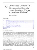
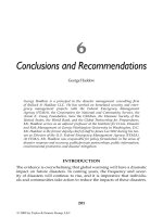
Figure 6.1 illustrates a situation where there are three observation
times before the impact, and four observation times after the impact.
Evidence for an impact is provided by a statistically significant change
in the difference between the control and impact sites before and after
the impact time. On the other hand, if the time plots for the two types
of sites remain approximately parallel, then there is no evidence that
the impact had an effect. Confidence in the existence of a lasting effect
is also gained if the time plots are approximately parallel before the
impact time, and then approximately parallel after the impact time, but
with the difference between them either increased or decreased.
It is possible, of course for an impact to have an effect that
increases or decreases with time. Figure 6.2 illustrates the latter
situation, where the impacted site apparently returns to its usual state
by about two time periods after the impact.

As emphasised by Underwood (1994), it is desirable to have more
than one control site to compare with the potentially impacted site, and
where possible these should be randomly selected from a population
of sites that are physically similar to the impact site. It is also important
to compare control sites to each other in order to be able to claim that
© 2001 by Chapman & Hall/CRC
the changes in the control sites reflect the changes that would be
present in the impact site if there were no effect of the impact.
Figure 6.1 A BACI study with three samples before and four samples after
the impact, which occurs between times 3 and 4.
Figure 6.2 A situation where the effect of an impact between times 3 and 4
becomes negligible after 4 time periods.
In experimental situations, there may be several impact sites as well
as several control sites. Clearly, the evidence of an impact from some
treatment is much improved if about the same effect is observed when
the treatment is applied independently in several different locations.
The analysis of BACI and other types of studies to assess the
impact of an event may be quite complicated because there are usually
repeated measurements taken over time at one or more sites. The
repeated measurements at one site will then often be correlated, with
those that are close in time tending to be more similar than those that
are further apart in time. If this correlation exists but is not taken into
account in the analysis of data, then the design has pseudoreplication
© 2001 by Chapman & Hall/CRC
(Section 4.8), with the likely result being that the estimated effects
appear to be more statistically significant than they should be.
When there are several control sites and several impact sites, each
measured several times before and several times after the time of the
impact, then one possibility is to use a repeated measures analysis of
variance. The form of the data would be as shown in Table 6.1, which

is for the case of three control and three impact sites, three samples
before the impact, and four samples after the impact. For a repeated
measures analysis of variance the two groups of sites give a single
treatment factor at two levels (control and impact), and one within site
factor which is the time relative to the impact, again at two levels
(before and after). The repeated measurements are the observations
at different times within the levels before and after, for one site. Interest
is in the interaction between treatment factor and the time relative to the
impact factor, because an impact will change the observations at the
impact sites but not the control sites.
Table 6.1 The form of results from a BACI experiment with three
observations before and four observations after the impact time.
Observations are indicated by X
Before the Impact After the Impact
Site Time 1 Time 2 Time 3 Time 4 Time 5 Time 6 Time 7
Control 1 X X X X X X X
Control 2 X X X X X X X
Control 3 X X X X X X X
Impact 1 X X X X X X X
Impact 2 X X X X X X X
Impact 3 X X X X X X X
There are other analyses that can be carried out on data of the form
shown in Table 6.1 that make different assumptions, and may be more
appropriate, depending on the circumstances (Von Ende, 1993).
Sometimes the data are obviously not normally distributed, or for some
other reason a generalized linear model approach as discussed in
Section 3.6 is needed rather than an analysis of variance. This is likely
to be the case, for example, if the observations are counts or
proportions. There are so many possibilities that it is not possible to
cover them all here, and expert advice should be sought unless the

appropriate analysis is very clear.
© 2001 by Chapman & Hall/CRC
Various analyses have been proposed for the situation where there
is only one control and one impact site (Manly, 1992, Chapter 6;
Rasmussen et al., 1993). In the next section a relatively straightforward
approach is described that may properly allow for serial correlation in
the observations from one site.
6.2 The Simple Difference Analysis with BACI Designs
Hurlebert (1984) highlighted the potential problem of pseudoreplication
with BACI designs due to the use of repeated observations from sites.
To overcome this, Stewart-Oaten et al. (1986) suggested that if
observations are taken at the same times at the control and impact
sites, then the differences between the impact and control sites at
different times may be effectively independent. For example, if the
control and impact sites are all in the same general area, then it can be
expected that they will be affected similarly by rainfall and other general
environmental factors. The hope is that by considering the difference
between the impact and control sites the effects of these general
environmental factors will cancel out.
This approach was briefly described in Example 1.4 on a large-scale
perturbation experiment. The following is another example of the same
type. Both of these examples involve only one impact site and one
control site. With multiple sites of each type the analysis can be
applied using the differences between the average for the impact sites
and the average for the control sites at different times.
Carpenter et al. (1989) considered the question of how much the
simple difference method is upset by serial correlation in the
observations from a site. As a result of a simulation study, they
suggested that to be conservative (in the sense of not declaring effects
to be significant more often than expected by chance) results that are

significant at a level of between 1% and 5% should be considered to be
equivocal. This was for a randomization test, but their conclusion is
likely to apply equally well to other types of test such as the t-test used
with Example 6.1.
Example 6.1 The Effect of Poison Pellets on Invertebrates
Possums (Trichosurus vulpecula) cause extensive damage in New
Zealand forests when their density gets high, and to reduce the
damage aerial drops of poison pellets containing 1080 (sodium
monofluoroacetate) poison are often made. The assumption is made
that the aerial drops have a negligible effect on non-target species, and
© 2001 by Chapman & Hall/CRC
a number of experiments have been carried out by the New Zealand
Department of Conservation to verify this.
One such experiment was carried out in 1997, with one control and
one impact site (McQueen and Lloyd, 2000). At the control site 100
non-toxic baits were put out on six occasions and the proportion of
these that were fed on by invertebrates was recorded for three nights.
At the impact site observations were taken in the same way on the
same six occasions, but for the last two occasions the baits were toxic,
containing 1080 poison. In addition, there was an aerial drop of poison
pellets in the impact area between the fourth and fifth sample times.
The question of interest was whether the proportion of baits being fed
on by invertebrates dropped in the impact area after the aerial drop. If
so, this may be result of the invertebrates being adversely affected by
the poison pellets.
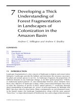
The available data are shown in Table 6.2, and plotted on Figure
6.3. The mean difference (impact - control) for times 1 to 4 before the
aerial drop is -0.138. The mean difference after the drop for times 5
and 6 is -0.150, which is very similar. Figure 6.3 also shows that the
time changes were rather similar at both sites, so there seems little

suggestion of an impact. Treating the impact - control differences
before the impact as a random sample of size 4, and the differences
after the impact as a random sample of size 2, the change in the mean
difference -0.150 - (-0.138) = -0.012 can be tested for significance
using a two-sample t-test. This gives t = -0.158 with 4 df, which is not
at all significant (p = 0.88 on a two-sided test). The conclusion must
therefore be that there is no evidence here of an impact resulting from
the aerial drop and the use of poison pellets.
If a significant difference had been obtained from this analysis it
would, of course, be necessary to consider the question of whether this
was just due to the time changes at the two sites being different for
reasons completely unrelated to the use of poison pellets at the impact
site. Thus the evidence for an impact would come down to a matter of
judgement in the end.
© 2001 by Chapman & Hall/CRC
Table 6.2 Results from an experiment to assess whether the
proportion of pellets fed on by invertebrates changes when the
pellets contain 1080 poison.
Time Control Impact Difference
1 0.40 0.37 -0.03
2 0.37 0.14 -0.23
3 0.56 0.40 -0.16
4 0.63 0.50 -0.13
Start of Impact
5 0.33 0.26 -0.07
6 0.45 0.22 -0.23
Mean Difference
Before -0.138
After -0.150
Figure 6.3 Results from a BACI experiment to see whether the proportion of

pellets fed on by invertebrates changes when there is an aerial drop of 1080
pellets at the impact site between times 4 and 5.
6.3 Matched Pairs with a BACI Design
When there is more than one impact site, pairing is sometimes used to
improve the study design, with each impact site being matched with a
control site that is as similar as possible. This is then called a control-
treatment paired (CTP) design (Skalski and Robson, 1992, Chapter 6),
or a before-after-control-impact-pairs (BACIP) design (Stewart-Oaten
et al., 1986). Sometimes information is also collected on variables that
describe the characteristics of the individual sites (elevation, slope,
etc.). These can then be used in the analysis of the data to allow for
© 2001 by Chapman & Hall/CRC
imperfect matching. The actual analysis depends on the procedure
used to select and match sites, and on whether or not variables to
describe the sites are recorded.
The use of matching can lead to a relatively straightforward analysis,
as demonstrated by the following example.
Example 6.2 Another Study of the Effect of Poison Pellets
Like Example 6.1, this concerns the effects of 1080 poison pellets on
invertebrates. However, the study design was rather different. The
original study is described by Sherley and Wakelin (1999). In brief, 13
separate trials of the use of 1080 were carried out, where for each trial
about 60 pellets were put out in a grid pattern in two adjacent sites,
over each of nine successive days. The pellets were of the type used
in aerial drops to reduce possum numbers. However, in one of the two
adjacent sites used for each trial the pellets never contained 1080
poison. This served as the control. In the other site the pellets
contained poison on days 4, 5 and 6 only. Hence the control and
impact sites were observed for three days before the impact, for three
days during the impact (1080 pellets), and for three days after the

impact was removed. The study carried out by Sherley and Wakelin
involved some other components as well as the nine day trials, but
these will not be considered here.
The average number of invertebrates seen on pellets each day is
shown in the top graph of Figure 6.4, for each of the 13 x 2 = 26 sites.
There is a great deal of variation in these averages, although it is
noticeable that the control sites tend to higher means, as well as being
more variable than the poison sites. When the results are averaged for
the control and poison sites, a clearer picture emerges (Figure 6.4,
bottom graph). The poison sites had slightly lower mean counts than
the control sites for days 1 to 3, the mean for the poison sites was
much lower for days 4 to 6, and then the difference became less for
days 7 to 9.
If the differences between the pairs of sites are considered, then the
situation becomes somewhat clearer (Figure 6.5). The poison sites
always had a lower mean than the control sites, but the difference
increased for days 4 to 6, and then started to return to the original level.
Once differences are taken, a result is available for each of the nine
days, for each of the 13 trials. An analysis of these differences is
possible using a two factor analysis of variance, as discussed in
Section 3.5. The two factors are the trial at 13 levels, and the day at
nine levels. As there is only one observation for each combination of
© 2001 by Chapman & Hall/CRC
these levels, it is not possible to estimate an interaction term, and the
model
x
ij
= µ + a
i
+ b

j
+ ,
ij
(6.1)
must be assumed, where x
ij
is the difference for trial i on day j, µ is an
overall mean, a
i
is an effect for the ith trial, b
j
is an effect for the jth day,
and ,
ij
represents random variation. When this model was fitted using
Minitab (Minitab Inc., 1994) the differences between trials were highly
significant (F = 8.89 with 12 and 96 df, p < 0.0005), as were the
differences between days (F = 9.26 with 8 and 96 df, p < 0.0005). It
appears, therefore, that there is very strong evidence that the poison
and control sites changed during the study, presumably because of the
impact of the 1080 poison.
There may be some concern that this analysis will be upset by serial
correlation in the results for the individual trials. However, this does not
seem to be a problem here because there are wide fluctuations from
day to day for some trials (Figure 6.5). Of more concern is the fact that
the standardized residuals (the differences between the observed
values for x and those predicted by the fitted model, divided by the
estimated standard deviation of the error term in the model) are more
variable for the larger predicted values (Figure 6.6). This seems to be
because the original counts of invertebrates on the pellets have a

variance that increases with the mean value of the count. This is not
unexpected because it is what usually occurs with counts, and a more
suitable analysis for the data involves fitting a log-linear model (Section
3.6) rather than an analysis of variance model. However, if a log-linear
model is fitted to the count data, then exactly the same conclusion is
reached: the difference between the poison and control sites changes
systematically over the nine days of the trials, with the number of
invertebrates decreasing during the three days of poisoning at the
treated sites, followed by some recovery towards the initial level in the
next three days.
This conclusion is quite convincing because of the replicated trials
and the fact that the observed impact has the pattern that is expected
if the 1080 poison has an effect on invertebrate numbers. The same
conclusion was reached by Sherley and Wakelin (1999) but using a
randomization test instead of analysis of variance or log-linear
modelling.
© 2001 by Chapman & Hall/CRC
Figure 6.4 Plots of the average number of invertebrates observed per pellet
(top graph) and the daily means (bottom graph) for the control areas (broken
lines) and the treated areas (continuous lines). At the treated site poison
pellets were used on days 4, 5 and 6 only.
© 2001 by Chapman & Hall/CRC
Figure 6.5 The differences between the poison and control sites for the 13
trials, for each day of the trials. The heavy line is the mean difference for all
trials. Poison pellets were used at the treated site for days 4, 5 and 6.
Figure 6.6 Plot of the standardized residuals from a two factor analysis of
variance against the values predicted by the model, for the difference
between the poison and control sites for one day of one trial.
© 2001 by Chapman & Hall/CRC
6.4 Impact-Control Designs

When there is an unexpected incident such as an oil spill there will
usually be no observations taken before the incident at either control or
impact sites. The best hope for impact assessment then is the impact-
control design, which involves comparing one or more potentially
impacted sites with similar control sites. The lack of 'before'
observations typically means that the design has low power in
comparison with BACI designs (Osenberg et al., 1994).
It is obvious that systematic differences between the control and
impact sites following the incident may be due to differences between
the types of sites rather than the incident. For this reason, it is
desirable to measure variables to describe the sites, in the hope that
these will account for much of the observed variation in the variables
that are used to describe the impact, if any.
Evidence of a significant area by time interaction is important in an
impact-control design, because this may be the only source of
information about the magnitude of an impact. For example, Figure 6.7
illustrates a situation where there is a large immediate effect of an
impact, followed by an apparent recovery to the situation where the
control and impact areas become rather similar.
Figure 6.7 The results from an impact-control study where an initial impact
at time 0 largely disappears by about time 4.
The analysis of the data from an impact-control study will obviously
depend on precisely how the data are collected. If there are a number
of control sites and a number of impact sites measured once each,
then the means for the two groups can be compared by a standard test
© 2001 by Chapman & Hall/CRC
of significance, and confidence limits for the difference can be
calculated. If each site is measured several times, then a repeated
measures analysis of variance may be appropriate. The sites are then
the 'subjects', with the two groups of sites giving two levels of a

treatment factor. As with the BACI design with multiple sites, careful
thought is needed to choose the best analysis for these types of data.
6.5 Before-After Designs
The before-after design can be used for situations where either no
suitable control areas exist, or it is not possible to measure suitable
areas. It does requires data to be collected before a potential impact
occurs, which may be the case with areas that are known to be
susceptible to damage, or which are being used for long-term
monitoring. The key question is whether the observations taken
immediately after an incident occurs can be considered to fit within the
normal range for the system. A pattern such as that shown in Figure
6.8 is expected, with a large change after the impact followed by a
return to normal conditions.
The analysis of the data must be based on some type of time series
analysis as discussed in Chapter 8 (Manly, 1992, Chapter 6;
Rasmussen et al., 1993). In simple cases where serial correlation in
the observations is negligible a multiple regression model may suffice.
However, if serial correlation is clearly present, then this should be
allowed for, possibly using a regression model with correlated errors
(Neter et al., 1983, Chapter 13).
Figure 6.8 The before-after design where an impact between times 2 and 3
disappears by about time 6.
© 2001 by Chapman & Hall/CRC
Of course, if some significant change is observed it is important to
be able to rule out causes other than the incident. For example, if an
oil spill occurs because of unusually bad weather, then the weather
itself may account for large changes in some environmental variables,
but not others.
6.6 Impact-Gradient Designs
The impact-gradient design can be used where there is a point source

of an impact, in areas that are fairly homogeneous. The idea is to
establish a function which demonstrates that the impact reduces as the
distance from the source of the impact increases. To this end, data are
collected at a range of distances from the source of the impact,
preferably with the largest distances being such that no impact is
expected. Regression methods can then be used to estimate the
average impact as a function of the distance from the source. There
may well be natural variation over the study area associated with the
type of habitat at different sample locations, in which case suitable
variables should be measured so that these can be included in the
regression equation to account for the natural variation as far as
possible.
A number of complications can occur with the analysis of data from
the impact-gradient design. The relationship between the impact and
the distance from the source may not be simple, necessitating the use
of non-linear regression methods, the variation in observations may not
be constant at different distances from the source, and there may be
spatial correlation, as discussed in Chapter 9. This is therefore another
situation where expert advice on the data analysis may be required.
6.7 Inferences from Impact Assessment Studies
'True' experiments as defined in Section 4.3 include randomization of
experimental units to treatments, replication to obtain observations
under the same conditions, and control observations that are obtained
under the same conditions as observations with some treatment
applied, but without any treatment. Most studies to assess
environmental impacts do not meet these conditions, and hence result
in conclusions that must be accepted with reservations. This does not
mean that the conclusions are wrong. It does mean that alternative
explanations for observed effects must be ruled out as unlikely to be
true.

© 2001 by Chapman & Hall/CRC
It is not difficult to devise alternative explanations for the simpler
study designs. With the impact-control design (Section 6.4) it is always
possible that the differences between the control and impact sites
existed before the time of the potential impact. If a significant
difference is observed after the time of the potential impact, and this is
claimed to be a true measure of the impact, then this can only be based
on the judgement that the difference is too large to be part of normal
variation. Likewise, with the before-after design (Section 6.5), if the
change from before to after the time of the potential impact is significant
and this is claimed to represent the true impact, then this is again
based on a judgement that the magnitude of the change is too large to
be explained by anything else. Furthermore, with these two designs no
amount of complicated statistical analysis can change these basic
weaknesses. In the social science literature these designs are
described as pre-experimental designs because they are not even as
good as quasi-experimental designs.
The BACI design with replication of control sites at least is better
because there are control observations in time (taken before the
potential impact) and in space (the sites with no potential impact).
However, the fact is that just because the control and impact sites have
an approximately constant difference before the time of the potential
impact it does not mean that this would necessarily continue in the
absence of an impact. If a significant change in the difference is used
as evidence of an impact, then it is an assumption that nothing else
could cause a change of this size.
Even the impact-gradient study design is not without its problems.
It might seem that a statistically significant trend in an environmental
variable with increasing distance from a potential point source of an
impact is clear evidence that the point source is responsible for the

change. However, the variable might naturally display spatial patterns
and trends associated with obvious and non-obvious physical
characteristics of the region. The probability of detecting a spurious
significant trend may then be reasonably high if this comes from an
analysis that does not take into account spatial correlation.
With all these limitations, it is possible to wonder about the value of
many studies to assess impacts. The fact is that they are often done
because they are all that can be done, and they give more information
than no study at all. Sometimes the estimated impact is so large that
it is impossible to imagine it being the result of anything but the impact
event, although some small part of the estimate may indeed be due to
natural causes. At other times the estimated impact is small and
insignificant, in which case it is not really possible to argue that
somehow the real impact is really large and important.
© 2001 by Chapman & Hall/CRC
6.8 Chapter Summary
The before-after-control-impact (BACI) study design is often used
to assess the impact of some event on variables that measure the
state of the environment. The design involves repeated
measurements over time being made at one or more control sites
and one or more potentially impacted sites, both before and after
the time of the event that may cause an impact.
Serial correlation in the measurements taken at a site results in
pseudoreplication if it is ignored in the analysis of data. Analyses
that may allow for this serial correlation in an appropriate way
include repeated measures analysis of variance.
A simple method that is valid with some sets of data takes the
differences between the observations at an impact site and a control
site, and tests for a significant change in the mean difference from
before the time of the potential impact to after this time. This

method can be applied using the differences between the mean for
several impact sites and the mean for several control sites. It is
illustrated using the results of an experiment on the effect of poison
pellets on invertebrate numbers.
A variation of the BACI design uses control and impact sites that are
paired up on the basis of their similarity. This can allow a relatively
simple analysis of the study results, as is illustrated by another study
on the effect of poison pellets on invertebrate numbers.
With an impact-control design, measurements at one or more
control sites are compared with measurements at one or more
impact sites only after the potential impact event has occurred.
With a before-after design, measurements are compared before and
after the time of the potential impact event, at impact sites only.
An impact-gradient study can be used when there is a point source
of a potential impact. This type of study looks for a trend in the
values of an environmental variable with increasing distance from
the point source.
Impact studies are not usually true experiments with randomization,
replication and controls. The conclusions drawn are therefore
based on assumptions and judgement. Nevertheless, they are often
© 2001 by Chapman & Hall/CRC
carried out because nothing else can be done and they are better
than no study at all.
© 2001 by Chapman & Hall/CRC