Modeling Hydrologic Change: Statistical Methods - Chapter 9 pot
Bạn đang xem bản rút gọn của tài liệu. Xem và tải ngay bản đầy đủ của tài liệu tại đây (466.95 KB, 37 trang )
Detection of Change
in Distribution
9.1 INTRODUCTION
Frequency analysis (see Chapter 5) is a univariate method of identifying a likely
population from which a sample was drawn. If the sample data fall near the fitted
line that is used as the best estimate of the population, then it is generally safe to use
the line to make predictions. However, “nearness to the line” is a subjective assess-
ment, not a systematic statistical test of how well the data correspond to the line.
That aspect of a frequency analysis is not objective, and individuals who have
different standards as to what constitutes a sufficiently good agreement may be at
odds on whether or not to use the fitted line to make predictions. After all, lines for
other distributions may provide a degree of fit that appears to be just as good. To
eliminate this element of subjectivity in the decision process, it is useful to have a
systematic test for assessing the extent to which a set of sample data agree with
some assumed population. Vogel (1986) provided a correlation coefficient test for
normal, log-normal, and Gumbel distributions.
The goal of this chapter is to present and apply statistical analyses that can be
used to test for the distribution of a random variable. For example, if a frequency
analysis suggested that the data could have been sampled from a lognormal distribu-
tion, one of the one-sample tests presented in this chapter could be used to decide
the statistical likelihood that this distribution characterizes the underlying population.
If the test suggests that it is unlikely to have been sampled from the assumed prob-
ability distribution, then justification for testing another distribution should be sought.
One characteristic that distinguishes the statistical tests from one another is the
number of samples for which a test is appropriate. Some tests are used to compare
a sample to an assumed population; these are referred to as one-sample tests. Another
group of tests is appropriate for comparing whether two distributions from which
two samples were drawn are the same, known as two-sample tests. Other tests are
appropriate for comparing samples from more than two distributions, referred to as
k
-sample tests.
9.2 CHI-SQUARE GOODNESS-OF-FIT TEST
The chi-square goodness-of-fit test is used to test for a significant difference between
the distribution suggested by a data sample and a selected probability distribution.
It is the most widely used one-sample analysis for testing a population distribution.
Many statistical tests, such as the
t
-test for a mean, assume that the data have been
9
L1600_Frame_C09.fm Page 209 Tuesday, September 24, 2002 3:26 PM
© 2003 by CRC Press LLC
drawn from a normal population, so it may be necessary to use a statistical test,
such as the chi-square test, to check the validity of the assumption for a given sample
of data. The chi-square test can also be used as part of the verification phase of
modeling to verify the population assumed when making a frequency analysis.
9.2.1 P
ROCEDURE
Data analysts are often interested in identifying the density function of a random
variable so that the population can be used to make probability statements about the
likelihood of occurrence of certain values of the random variable. Very often, a
histogram plot of the data suggests a likely candidate for the population density
function. For example, a frequency histogram with a long right tail might suggest
that the data were sampled from a lognormal population. The chi-square test for
goodness of fit can then be used to test whether the distribution of a random variable
suggested by the histogram shape can be represented by a selected theoretical
probability density function (PDF). To demonstrate the quantitative evaluation, the
chi-square test will be used to evaluate hypotheses about the distribution of the
number of storm events in 1 year, which is a discrete random variable.
Step 1: Formulate hypotheses
. The first step is to formulate both the null (
H
0
)
and the alternative (
H
A
) hypotheses that reflect the theoretical density func-
tion (PDF; continuous random variables) or probability mass function (PMF;
discrete random variables). Because a function is not completely defined
without the specification of its parameters, the statement of the hypotheses
must also include specific values for the parameters of the function. For
example, if the population is hypothesized to be normal, then
µ
and
σ
must
be specified; if the hypotheses deal with the uniform distribution, values
for the location
α
and scale
β
parameters must be specified. Estimates of
the parameters may be obtained either empirically or from external condi-
tions. If estimates of the parameters are obtained from the data set used in
testing the hypotheses, the degrees of freedom must be modified to reflect this.
General statements of the hypotheses for the chi-square goodness-of-fit
test of a continuous random variable are:
H
0
:
X
∼
PDF (stated values of parameters) (9.1a)
H
A
:
X
≠
PDF (stated values of parameters) (9.1b)
If the random variable is a discrete variable, then the PMF replaces the PDF.
The following null and alternative hypotheses are typical:
H
0
: The number of rainfall events that exceed 1 cm in any year at a particular
location can be characterized by a uniform density function with a loca-
tion parameter of zero and a scale parameter of 40.
H
A
: The uniform population
U
(0, 40) is not appropriate for this random
variable.
L1600_Frame_C09.fm Page 210 Tuesday, September 24, 2002 3:26 PM
© 2003 by CRC Press LLC
Mathematically, these hypotheses are
H
0
:
f
(
n
)
=
U(
α
=
0,
β
=
40) (9.2a)
H
A
:
f
(
n
)
≠
U(
α
=
0,
β
=
40) (9.2b)
Note specifically that the null hypothesis is a statement of equality and the
alternative hypothesis is an inequality. Both hypotheses are expressed in
terms of population parameters, not sample statistics.
Rejection of the null hypothesis would not necessarily imply that the ran-
dom variable is not uniformly distributed. It may also be rejected because
one or both of the parameters, in this case 0 and 40, are incorrect. Rejection
may result because the assumed distribution is incorrect, one or more of the
assumed parameters is incorrect, or both.
The chi-square goodness-of-fit test is always a one-tailed test because the
structure of the hypotheses are unidirectional; that is, the random variable is
either distributed as specified in the null hypothesis or it is not.
Step 2: Select the appropriate model.
To test the hypotheses formulated in
step 1, the chi-square test is based on a comparison of the observed fre-
quencies of values in the sample with frequencies expected with the PDF
of the population, which is specified in the hypotheses. The observed data
are typically used to form a histogram that shows the observed frequencies
in a series of
k
cells. The cell bounds are often selected such that the cell
width for each cell is the same; however, unequal cell widths could be
selected to ensure a more even distribution of the observed and expected
frequencies. Having selected the cell bounds and counted the observed
frequencies for cell
i
(
O
i
), the expected frequencies
E
i
for each cell can be
computed using the PDF of the population specified in the null hypothesis
of step 1. To compute the expected frequencies, the expected probability
for each cell is determined for the assumed population and multiplied by
the sample size
n
. The expected probability for cell
i
,
p
i
, is the area under
the PDF between the cell bounds for that cell. The sum of the expected
frequencies must equal the total sample size
n
. The frequencies can be
summarized in a cell structure format, such as Figure 9.1a.
The test statistic, which is a random variable, is a function of the observed
and expected frequencies, which are also random variables:
(9.3)
where
χ
2
is the computed value of a random variable having a chi-square
distribution with
ν
degrees of freedom;
O
i
and
E
i
are the observed and ex-
pected frequencies in cell
i
, respectively; and
k
is the number of discrete cat-
egories (cells) into which the data are separated. The random variable
χ
2
has
χ
2
2
1
=
−
=
∑
()OE
E
ii
i
i
k
L1600_Frame_C09.fm Page 211 Tuesday, September 24, 2002 3:26 PM
© 2003 by CRC Press LLC
a sampling distribution that can be approximated by the chi-square distribu-
tion with
k
−
j
degrees of freedom, where
j
is the number of quantities that
are obtained from the sample of data for use in calculating the expected fre-
quencies. Specifically, since the total number of observations
n
is used to
compute the expected frequencies, 1 degree of freedom is lost. If the mean
and standard deviation of the sample are needed to compute the expected
frequencies, then two additional degrees of freedom are subtracted (i.e.,
υ
=
k
−
3). However, if the mean and standard deviation are obtained from past
experience or other data sources, then the degrees of freedom for the test sta-
tistic remain
υ
=
k
−
1. It is important to note that the degrees of freedom do
not directly depend on the sample size
n
; rather they depend on the number
of cells.
Step 3: Select the level of significance
. If the decision is not considered critical,
a level of significance of 5% may be considered appropriate, because of
convention. A more rational selection of the level of significance will be
discussed later. For the test of the hypotheses of Equation 9.2, a value of
5% is used for illustration purposes.
Step 4: Compute estimate of test statistic
. The value of the test statistic of
Equation 9.3 is obtained from the cell frequencies of Figure 9.1b. The range
of the random variable was separated into four equal intervals of ten. Thus,
the expected probability for each cell is 0.25 (because the random variable
is assumed to have a uniform distribution and the width of the cells is the
same). For a sample size of 80, the expected frequency for each of the four
cells is 20 (i.e., the expected probability times the total number of observa-
tions). Assume that the observed frequencies of 18, 19, 25, and 18 are deter-
mined from the sample, which yields the cell structure shown in Figure 9.1b.
FIGURE 9.1
Cell structure for chi-square goodness-of-fit test: (a) general structure; and (b)
structure for the number of rainfall events.
Cell bound −∞ . . . .
Cell number i 1 2 3 . . . . k
Observed frequency (O
i
) O
1
O
2
O
3
. . . . O
k
Expected frequency (E
i
) E
1
E
2
E
3
. . . . E
k
(O
i
– E
i
)
2
/E
i
. . . .
(a)
Cell bound 0 10 20 30 40
Cell number i 1234
Observed frequency (O
i
)18192518
Expected frequency (E
i
)20202020
(O
i
– E
i
)
2
/E
i
0.20 0.05 1.25 0.20
(b)
()OE
E
11
2
1
− ()OE
E
22
2
2
−
()OE
E
33
2
3
−
()OE
E
kk
k
−
2
L1600_Frame_C09.fm Page 212 Tuesday, September 24, 2002 3:26 PM
© 2003 by CRC Press LLC
Using Equation 9.3, the computed statistic
χ
2
equals 1.70. Because the total
frequency of 80 was separated into four cells for computing the expected
frequencies, the number of degrees of freedom is given by
υ
=
k
−
1, or
4
−
1
=
3.
Step 5: Define the region of rejection
. According to the underlying theorem
of step 2, the test statistic has a chi-square distribution with 3 degrees of
freedom. For this distribution and a level of significance of 5%, the critical
value of the test statistic is 7.81 (Table A.3). Thus, the region of rejection
consists of all values of the test statistic greater than 7.81. Note again, that
for this test the region of rejection is always in the upper tail of the chi-
square distribution.
Step 6: Select the appropriate hypothesis
. The decision rule is that the null
hypothesis is rejected if the chi-square value computed in step 4 is larger
than the critical value of step 5. Because the computed value of the test
statistic (1.70) is less than the critical value (7.81), it is not within the
region of rejection; thus the statistical basis for rejecting the null hypothesis
is not significant. One may then conclude that the uniform distribution with
location and scale parameters of 0 and 40, respectively, may be used to
represent the distribution of the number of rainfall events. Note that other
distributions could be tested and found to be statistically acceptable, which
suggests that the selection of the distribution to test should not be an arbitrary
decision.
In summary, the chi-square test for goodness of fit provides the means for
comparing the observed frequency distribution of a random variable with a popula-
tion distribution based on a theoretical PDF or PMF. An additional point concerning
the use of the chi-square test should be noted. The effectiveness of the test is
diminished if the expected frequency in any cell is less than 5. When this condition
occurs, both the expected and observed frequencies of the appropriate cell should
be combined with the values of an adjacent cell; the value of
k
should be reduced
to reflect the number of cells used in computing the test statistic. It is important to
note that this rule is based on expected frequencies, not observed frequencies.
To illustrate this rule of thumb, consider the case where observed and expected
frequencies for seven cells are as follows:
Note that cells 3 and 7 have expected frequencies less than 5, and should,
therefore, be combined with adjacent cells. The frequencies of cell 7 can be combined
with the frequencies of cell 6. Cell 3 could be combined with either cell 2 or cell
4. Unless physical reasons exist for selecting which of the adjacent cells to use, it
is probably best to combine the cell with the adjacent cell that has the lowest expected
Cell 1234 567
O
i
3975 946
E
i
68461072
L1600_Frame_C09.fm Page 213 Tuesday, September 24, 2002 3:26 PM
© 2003 by CRC Press LLC
frequency count. Based on this, cells 3 and 4 would be combined. The revised cell
configuration follows:
The value of
k
is now 5, which is the value to use in computing the degrees
of freedom. Even though the observed frequency in cell 1 is less than 5, that cell is
not combined. Only expected frequencies are used to decide which cells need to be
combined. Note that a cell count of 5 would be used to compute the degrees of
freedom, rather than a cell count of 7.
9.2.2 C
HI
-S
QUARE
T
EST
FOR
A
N
ORMAL
D
ISTRIBUTION
The normal distribution is widely used because many data sets have shown to have
a bell-shaped distribution and because many statistical tests assume the data are
normally distributed. For this reason, the test procedure is illustrated for data assumed
to follow a normal population distribution.
Example 9.1
To illustrate the use of the chi-square test with the normal distribution, a sample of
84 discharges is used. The histogram of the data is shown in Figure 9.2. The sample
mean and standard deviation of the random variable were 10,100, and 780, respec-
tively. A null hypothesis is proposed that the random variable is normally distributed
with a mean and standard deviation of 10,100 and 780, respectively. Note that the
sample moments are being used to define the population parameters in the statement
of hypotheses; this will need to be considered in the computation of the degrees of
freedom. Table 9.1 gives the cell bounds used to form the observed and expected
frequency cells (see column 2). The cell bounds are used to compute standardized
Cell 1 2 3 4 5
O
i
3 9 12 9 10
E
i
6 8 10 10 9
FIGURE 9.2
Histogram of discharge rate (
Q
, cfs).
8000
9000 10,000 11.000 12,000
Q
12
4
20
24
13
7
4
L1600_Frame_C09.fm Page 214 Tuesday, September 24, 2002 3:26 PM
© 2003 by CRC Press LLC
TABLE 9.1
Computations for Example 9.1
Cell i
Cell
Bound z
i
P(z < z
i
)
Expected
Probability
Expected
Frequency
Observed
Frequency
1 9000 0.0793 0.0793 6.66 12
2 9500 0.2206 0.1413 11.87 4
3 10,000 0.4483 0.2277 19.13 20
4 10,500 0.6985 0.2502 21.02 24
5 11,000 0.8749 0.1764 14.82 13
6 11,500 0.9633 0.0884 11
7 ∞
1.0000 84 84 10.209
()
2
OE
E
ii
i
−
9000 10 100
780
141
−
=−
,
.
(.)
.
.
12 6 66
666
4 282
2
−
=
9500 10 100
780
077
−
=−
,
.
(.)
.
.
41187
11 87
5 218
2
−
=
10 000 10 100
780
013
,,
.
−
=−
(.)
.
.
20 19 13
19 13
0 040
2
−
=
10 500 10 100
780
052
,,
.
−
=
(.)
.
.
24 21 02
21 02
0 422
2
−
=
11 000 10 100
780
115
,,
.
−
=
(.)
.
.
13 14 82
14 82
0 224
2
−
=
11 500 10 100
780
179
,,
.
−
=
742
308
10 50
.
.
.
(.)
.
.
11 10 50
10 50
0 024
2
−
=
0 0367
1 0000
.
.
L1600_Frame_C09.fm Page 215 Tuesday, September 24, 2002 3:26 PM
© 2003 by CRC Press LLC
variates z
i
for the bounds of each interval (column 3), the probability that the variate
z is less than z
i
(column 4), the expected probabilities for each interval (column 5),
the expected and observed frequencies (columns 6 and 7), and the cell values of the
chi-square statistic of Equation 9.3 (column 8).
The test statistic has a computed value of 10.209. Note that because the expected
frequency for the seventh interval was less than 5, both the observed and expected
frequencies were combined with those of the sixth cell. Three degrees of freedom
are used for the test. With a total of six cells, 1 degree of freedom was lost for n,
while two were lost for the mean and standard deviation, which were obtained
from the sample of 84 observations. (If past evidence had indicated a mean of
10,000 and a standard deviation of 1000, and these statistics were used in Table 9.1
for computing the expected probabilities, then 5 degrees of freedom would be
used.) For a level of significance of 5% and 3 degrees of freedom, the critical chi-
square value is 7.815. The null hypothesis is, therefore, rejected because the
computed value is greater than the critical value. One may conclude that discharges
on this watershed are not normally distributed with
µ
= 10,100 and
σ
= 780. The
reason for the rejection of the null hypothesis may be due to one or more of the
following: (1) the assumption of a normal distribution is incorrect, (2)
µ
≠ 10,100,
or (3)
σ
≠ 780.
Alternative Cell Configurations
Cell boundaries are often established by the way the data were collected. If a data
set is collected without specific bounds, then the cell bounds for the chi-square test
cells can be established at any set of values. The decision should not be arbitrary,
especially with small sample sizes, since the location of the bounds can influence
the decision. For small and moderate sample sizes, multiple analyses with different
cell bounds should be made to examine the sensitivity of the decision to the place-
ment of the cell bounds.
While any cell bounds can be specified, consider the following two alternatives:
equal intervals and equal probabilities. For equal-interval cell separation, the cell
bounds are separated by an equal cell width. For example, test scores could be
separated with an interval of ten: 100–90, 90–80, 80–70, and so on. Alternatively,
the cell bounds could be set such that 25% of the underlying PDF was in each
cell. For the standard normal distribution N(0, 1) with four equal-probability cells,
the upper bounds of the cells would have z values of −0.6745, 0.0, 0.6745, and ∞.
The advantage of the equal-probability cell alternative is that the probability can
be set to ensure that the expected frequencies are at least 5. For example, for a
sample size of 20, 4 is the largest number of cells that will ensure expected
frequencies of 5. If more than four cells are used, then at least 1 cell will have an
E
i
of less than 5.
Comparison of Cell Configuration Alternatives
The two-cell configuration alternatives can be used with any distribution. This will
be illustrated using the normal distribution.
L1600_Frame_C09.fm Page 216 Tuesday, September 24, 2002 3:26 PM
© 2003 by CRC Press LLC
Example 9.2
Consider the total lengths of storm-drain pipe used on 70 projects (see Table B.6).
The pipe-length values have a mean of 3096 ft and a standard deviation of 1907 ft.
The 70 lengths are allocated to eight cells using an interval of 1000 ft (see Table 9.2
and Figure 9.3a). The following hypotheses will be tested:
Pipe length ~ N(
µ
= 3096,
σ
= 1907) (9.4a)
Pipe length ≠ N(3096, 1907) (9.4b)
Note that the sample statistics are used to define the hypotheses and will, therefore,
be used to compute the expected frequencies. Thus, 2 degrees of freedom will be
subtracted because of their use. To compute the expected probabilities, the standard
normal deviates z that correspond to the upper bounds X
u
of each cell are computed
(see column 4 of Table 9.2) using the following transformation:
(9.5)
The corresponding cumulative probabilities are computed from the cumulative
standard normal curve (Table A.1) and are given in column 5. The probabilities
associated with each cell (column 6) are taken as the differences of the cumulative
probabilities of column 5. The expected frequencies (E
i
) equal the product of the
sample size 70 and the probability p
i
(see column 7). Since the expected frequencies
in the last two cells are less than 5, the last three cells are combined, which yields
six cells. The cell values of the chi-square statistic of Equation 9.3 are given in
column 8, with a sum of 22.769. For six cells with 3 degrees of freedom lost, the
TABLE 9.2
Chi-Square Test of Pipe Length Data Using Equal Interval Cells
Cell
Length (ft)
Range
Observed
Frequency,
O
i
z
i
∑p
i
p
i
E
i
==
==
np
i
10–1000 3 −1.099 0.1358 0.1358 9.506 4.453
2 1000–2000 20 −0.574 0.2829 0.1471 10.297 9.143
3 2000–3000 22 −0.050 0.4801 0.1972 13.804 4.866
4 3000–4000 8 0.474 0.6822 0.2021 14.147 2.671
5 4000–5000 7 0.998 0.8409 0.1587 11.109 1.520
6 5000–6000 2 1.523 0.9361 0.0952 0.116
7
6000–7000 3 2.047 0.9796 0.0435 11.137 0
8
7000–∞ 5 ∞ 1.0000 0.0204 0
70 70.000 22.769
()
2
OE
E
ii
i
−
6.664
3.045
1.428
z
XX
S
X
u
x
u
=
−
=
− 3096
1907
L1600_Frame_C09.fm Page 217 Tuesday, September 24, 2002 3:26 PM
© 2003 by CRC Press LLC
critical test statistic for a 5% level of significance is 7.815. Thus, the computed value
is greater than the critical value, so the null hypothesis can be rejected. The null
hypothesis would be rejected even at a 0.5% level of significance ( ).
Therefore, the distribution specified in the null hypothesis is unlikely to characterize
the underlying population.
For a chi-square analysis using the equal-probability alternative, the range is
divided into eight cells, each with a probability of 1/8 (see Figure 9.3b). The
cumulative probabilities are given in column 1 of Table 9.3. The z
i
values (column
2) that correspond to the cumulative probabilities are obtained from the standard
normal table (Table A.1). The pipe length corresponding to each z
i
value is computed
by (see column 3):
X
u
=
µ
+ z
i
σ
= 3096 + 1907z
i
(9.6)
These upper bounds are used to count the observed frequencies (column 4) from
the 70 pipe lengths. The expected frequency (E
i
) is np = 70(1/8) = 8.75. Therefore,
the computed chi-square statistic is 18.914. Since eight cells were used and 3 degrees
FIGURE 9.3 Frequency histogram of pipe lengths (L, ft × 10
3
) using (a) equals interval and
(b) equal probability cells.
01234567
8
01234567
8
3
17
12
13
6
5
5
9
3
20
22
8
7
2
3
5
(a)
(b)
L
L
χ
.
.
005
2
12 84=
L1600_Frame_C09.fm Page 218 Tuesday, September 24, 2002 3:26 PM
© 2003 by CRC Press LLC
of freedom were lost, the critical value for a 5% level of significance and 5 degrees
of freedom is 11.070. Since the computed value exceeds the critical value, the null
hypothesis is rejected, which suggests that the population specified in the null
hypothesis is incorrect.
The computed value of chi-square for the equal-probability delineation of cell
bounds is smaller than for the equal-cell-width method. This occurs because the
equal-cell-width method causes a reduction in the number of degrees of freedom,
which is generally undesirable, and the equal-probability method avoids cells with
a small expected frequency. Since the denominator of Equation 9.3 acts as a weight,
low expected frequencies contribute to larger values of the computed chi-square
value.
9.2.3 CHI-SQUARE TEST FOR AN EXPONENTIAL DISTRIBUTION
The histogram in Figure 9.4 has the general shape of an exponential decay function,
which has the following PDF:
ƒ(x) =
λ
e
−
λ
x
for x > 0 (9.7)
in which
λ
is the scale parameter and x is the random variable. It can be shown that
the method of moments estimator of
λ
is the reciprocal of the mean (i.e.,
λ
= ).
Probabilities can be evaluated by integrating the density function f(x) between the
upper and lower bounds of the interval. Intervals can be set randomly or by either
the constant-probability or constant-interval method.
Example 9.3
Using the sediment yield Y data of Table B.1 and the histogram of Figure 9.4, a test
was made for the following hypotheses:
TABLE 9.3
Chi-Square Test of Pipe Length Data Using Equal
Probability Cells
∑pX XO
i
X
i
0.125 −1.150 903 3 70/8 3.779
0.250 −0.675 1809 17 70/8 7.779
0.375 −0.319 2488 12 70/8 1.207
0.500 0.000 3096 13 70/8 2.064
0.625 0.319 3704 6 70/8 0.864
0.750 0.675 4383 5 70/8 1.607
0.875 1.150 5289 5 70/8 1.607
1.000 ∞∞9 70/8
0.007
18.914
1/ x
L1600_Frame_C09.fm Page 219 Tuesday, September 24, 2002 3:26 PM
© 2003 by CRC Press LLC
H
o
: Y has an exponential density function with
(9.8)
H
A
: Y is not exponentially distributed, with
The calculation of the computed value of chi-square is shown in Table 9.4. Although
the histogram initially included five cells, the last three cells had to be combined to
ensure that all cells would have an expected frequency of 5 or greater. The computed
TABLE 9.4
Computations for Example 9.3
Cell Interval f(x)
Expected
Nf(x)
Observed
O
i
|d
i
|
1
0 ≤ x ≤ 0.35125 0.4137 15.30 22 6.70 2.93
2
0.35125 ≤ x ≤ 1.01375 0.3721 13.77 7 6.77 3.33
3
1.01375 ≤ x ≤ 1.67625 0.1359
4
1.67625 ≤ x ≤ 2.33875 0.0497 0.07 0.00
5
2.33875 ≤ x 0.0286
1.0000 37.00 37 6.263
FIGURE 9.4 Histogram of sediment yield data.
de
ii
2
/
5.03
1.84
1.06
793.
3
2
3
8
22
20
18
16
14
12
10
8
6
4
2
0
021
Sediment yield
Frequency
0.35125
Mean
1.01375
1.67625
2.33875
2.67
7
22
3
2
3
n
= 37
ˆ
.
.
λ
== =
11
0 6579
1 520
Y
ˆ
.
λ
= 152
L1600_Frame_C09.fm Page 220 Tuesday, September 24, 2002 3:26 PM
© 2003 by CRC Press LLC
chi-square statistic is 6.263. Two degrees of freedom are lost because n and were
used to compute the expected frequencies; therefore, with only three cells, only 1
degree of freedom remains. For levels of significance of 5% and 1% and 1 degree
of freedom, the critical values are 3.841 and 6.635, respectively. Thus, the null
hypothesis would be rejected for a 5% level of significance but accepted for 1%.
This illustrates the importance of selecting the level of significance on the basis of
a rational analysis of the importance of type I and II errors.
9.2.4 CHI-SQUARE TEST FOR LOG-PEARSON III DISTRIBUTION
The log-Pearson type III distribution is used almost exclusively for the analysis of
flood peaks. Whether the data points support the use of a log-Pearson III distribution
is usually a subjective decision based on the closeness of the data points to the
assumed population curve. To avoid this subjectivity, a statistical analysis may be a
good alternative in determining whether the data points support the assumed LP3
distribution. The chi-square test is one possible analysis. Vogel’s (1986) probability
plot correlation coefficient is an alternative.
Two options are available for estimating probabilities. First, the LP3 density
function can be integrated between cell bounds to obtain probabilities to compute
the expected frequencies. Second, the tabular relationship between the exceedance
probability and the LP3 deviates K can be applied. The first option would enable
the use of the constant probability method for setting cell bounds; however, it would
require the numerical integration of the LP3 density function. The second option
has the disadvantage that getting a large number of cells may be difficult. The second
option is illustrated in the following example.
Example 9.4
The 38-year record of annual maximum discharges for the Back Creek watershed
(Table B.4) is used to illustrate the application of the chi-square test with the LP3
distribution. The 32-probability table of deviates (Table A.11) is used to obtain the
probabilities for each cell. The sample skew is −0.731; therefore, the K values for
a skew of −0.7 are used with the sample log mean of 3.722 and sample log standard
deviation of 0.2804 to compute the log cell bound X (column 3 of Table 9.5) and
the cell bound Y (column 4):
X = 3.722 + 0.2804 K (9.9a)
Y = 10
X
(9.9b)
The cell bounds Y are used to compute the observed frequencies O
i
(column 5). The
cumulative probability of column 1 is incremented to get the cell probabilities of
column 6, which are multiplied by the sample size n to compute the expected
frequencies E
i
(column 7). Cells must be combined to ensure that the expected cell
frequencies are at least 5. Table 9.6 gives the results of the chi-square test. The
computed chi-square value is 8.05. Since the three sample moments and the sample
Y
L1600_Frame_C09.fm Page 221 Tuesday, September 24, 2002 3:26 PM
© 2003 by CRC Press LLC
size were used to estimate the expected probabilities, 4 degrees of freedom are lost.
With 5 cells, only 1 degree of freedom is available. The critical chi-square values
for 5%, 1%, and 0.5% levels of significance are 3.84, 6.63, and 7.88, respectively.
Therefore, the null hypothesis of an LP3 PDF must be rejected:
H
O
: Y ~ LP3 (log
µ
= 3.722, log
σ
= 0.2804, log g = −0.7) (9.10)
TABLE 9.5
Chi-Square Test for Log-Pearson III Distribution
∑PK Y = 10
X
O
i
p
i
e
i
= np
i
Sample
Probability Difference
0.0001 −5.274 2.243 175 0 0.0001 0.0038 0.0001
0.0005 −4.462 2.471 296 0 0.0004 0.0152 0.0004
0.0010 −4.100 2.572 374 0 0.0005 0.0190 0.0005
0.0020 −3.730 2.676 474 0 0.0010 0.0380 0.0010
0.0050 −3.223 2.818 658 1 0.0030 0.1140 1/38 −0.0243
0.0100 −2.824 2.930 851 0 0.0050 0.1900 −0.0213
0.0200 −2.407 3.047 1114 0 0.0100 0.3800 −0.0163
0.0250 −2.268 3.086 1219 0 0.0050 0.1900 −0.0063
0.0400 −1.967 3.170 1481 0 0.0150 0.5700 −0.0013
0.0500 −1.819 3.212 1629 1 0.0100 0.3800 2/38 −0.0126
0.1000 −1.333 3.348 2230 0 0.0500 1.9000 −0.0026
0.2000 −0.790 3.500 3166 2 0.1000 3.8000 4/38 −0.0053
0.3000 −0.429 3.602 3997 6 0.1000 3.8000 10/38 −0.0632
0.4000 −0.139 3.683 4820 8 0.1000 3.8000 18/38 −0.1739
0.4296 −0.061 3.705 5068 1 0.0296 1.1248 19/38 −0.1000
0.5000 0.116 3.755 5682 4 0.0704 2.6752 23/38 −0.1757
0.5704 0.285 3.802 6337 2 0.0704 2.6752 25/38 −0.1579
0.6000 0.356 3.822 6635 0 0.0296 1.1248 25/38 −0.0875
0.7000 0.596 3.889 7747 4 0.1000 3.8000 29/38 −0.0632
0.8000 0.857 3.962 9168 4 0.1000 3.8000 33/38 −0.0684
0.9000 1.183 4.054 11317 2 0.1000 3.8000 35/38 −0.0211
0.9500 1.423 4.121 13213 0 0.0500 1.9000 0.0289
0.9600 1.489 4.140 13788 0 0.0100 0.3800 0.0389
0.9750 1.611 4.174 14918 0 0.0150 0.5700 0.0539
0.9800 1.663 4.188 15428 0 0.0050 0.1900 0.0589
0.9900 1.806 4.228 16920 1 0.0100 0.3800 36/38 0.0426
0.9950 1.926 4.262 18283 0 0.0050 0.1900 0.0476
0.9980 2.057 4.299 19897 1 0.0030 0.1140 37/38 0.0243
0.9990 2.141 4.322 21006 0 0.0010 0.0380 0.0253
0.9995 2.213 4.343 22005 0 0.0005 0.0190 0.0258
0.9999 2.350 4.381 24040 1 0.0004 0.0152 38/38 −0.0001
1.0000 —— ——0.0001 0.0038 0.0000
38 1.0000 38.0000
XXKS=+
L1600_Frame_C09.fm Page 222 Tuesday, September 24, 2002 3:26 PM
© 2003 by CRC Press LLC
It appears that either the LP3 distribution is not appropriate or one or more of the
sample parameters are not correct. Note that, if the LP3 deviates K are obtained
from the table (Table A.11), then neither the equal probability or the equal cell width
is used. In this case, the cell bounds are determined by the probabilities in the table.
9.3 KOLMOGOROV–SMIRNOV ONE-SAMPLE TEST
A frequent problem in data analysis is verifying that the population can be repre-
sented by some specified PDF. The chi-square goodness-of-fit test was introduced
as one possible statistical test; however, the chi-square test requires at least a mod-
erate sample size. It is difficult to apply the chi-square test with small samples
because of the 5-or-greater expected frequency limitation. Small samples will lead
to a small number of degrees of freedom. The Kolmogorov–Smirnov one-sample
(KS1) test was developed for verifying a population distribution and can be used
with much smaller samples than the chi-square test. It is considered a nonparametric
test.
9.3.1 PROCEDURE
The KS1 tests the null hypothesis that the cumulative distribution of a variable agrees
with the cumulative distribution of some specified probability function; the null
hypothesis must specify the assumed population distribution function and its param-
eters. The alternative hypothesis is accepted if the distribution function is unlikely
to be the underlying function; this may be indicated if either the density function
or the specified parameters is incorrect.
The test statistic, which is denoted as D, is the maximum absolute difference
between the values of the cumulative distributions of a random sample and a specified
probability distribution function. Critical values of the test statistic are usually
available only for limited values of the level of significance; those for 5% and 1%
are given in Table A.12.
The KS1 test may be used for small samples; it is generally more efficient than
the chi-square goodness-of-fit test when the sample size is small. The test requires
TABLE 9.6
Chi-Square Test for Log-Pearson III
Distribution
Cells E
i
O
i
(O
i
− E
i
)
2
/E
i
0–3166 7.6 4 1.705
3167–4820 7.6 14 5.389
4821–6635 7.6 7 0.047
6636–9168 7.6 8 0.021
9169–∞ 7.6 5 0.889
38.0 38 8.051
L1600_Frame_C09.fm Page 223 Tuesday, September 24, 2002 3:26 PM
© 2003 by CRC Press LLC
data on at least an ordinal scale, but it is applicable for comparisons with continuous
distributions. (The chi-square test may also be used with discrete distributions.)
The Kolmogorov–Smirnov one-sample test is computationally simple; the com-
putational procedure requires the following six steps:
1. State the null and alternative hypotheses in terms of the proposed PDF
and its parameters. Equations 9.1 are the two hypotheses for the KS1 test.
2. The test statistic, D, is the maximum absolute difference between the
cumulative function of the sample and the cumulative function of the
probability function specified in the null hypothesis.
3. The level of significance should be set; values of 0.05 and 0.01 are
commonly used.
4. A random sample should be obtained and the cumulative probability
function derived for the sample data. After computing the cumulative
probability function for the assumed population, the value of the test
statistic can be computed.
5. The critical value, D
α
, of the test statistic can be obtained from tables of
D
α
in Table A.12. The value of D
α
is a function of
α
and the sample size, n.
6. If the computed value D is greater than the critical value D
α
, the null
hypothesis should be rejected.
When applying the KS1 test, it is best to use as many cells as possible. For small
and moderate sample sizes, each observation can be used to form a cell. Maximizing
the number of cells increases the likelihood of finding a significant result if the null
hypothesis is, in fact, incorrect. Thus, the probability of making a type I error is
minimized.
Example 9.5
The following are estimated erosion rates (tons/acre/year) from 13 construction
sites:
The values are to be compared with a study that suggested erosion rates could be
represented by a normal PDF with a mean and standard deviation of 55 and 5,
respectively. If a level of significance of 5% is used, would it be safe to conclude
that the sample is from a normally distributed population with a mean of 55 and a
standard deviation of 5?
If the data are separated on a scale with intervals of 5 tons/acre/year, the
frequency distribution (column 2), sample probability function (column 3), and
population probability function (column 4) are as given in Table 9.7. The cumulative
function for the population uses the z transform to obtain the probability values; for
example, the z value for the upper limit of the first interval is
(9.11)
47 53 61 57 64 44 56 52 63 58 49 51 54
z =
−
=−
45 55
5
2
L1600_Frame_C09.fm Page 224 Tuesday, September 24, 2002 3:26 PM
© 2003 by CRC Press LLC
Thus, the probability is p(z < −2) = 0.0228. After the cumulative functions were
derived, the absolute difference was computed for each range. The value of the test
statistic, which equals the largest absolute difference, is 0.0721. For a 5% level of
significance, the critical value (see Table A.12) is 0.361. Since the computed value
is less than D
α
, the null hypothesis cannot be rejected.
With small samples, it may be preferable to create cells so that each cell contains
a single observation. Such a practice will lead to the largest possible difference
between the cumulative distributions of the sample and population, and thus the
greatest likelihood of rejecting the null hypothesis. This is a recommended practice.
To illustrate this, the sample of 13 was separated into 13 cells and the KS1 test
applied (see Table 9.8). With one value per cell, the observed cumulative probabilities
would increase linearly by 1/13 per cell (see column 4). The theoretical cumulative
probabilities (see column 3) based on the null hypothesis of a normal distribution
(
µ
= 55,
σ
= 5) are computed by z = (x − 55)/5 (column 2). Column 5 of Table 9.8
TABLE 9.7
Example of Kolmogorov–Smirnov One-Sample Test
Range
Observed
Frequency
Probability
Function
Cumulative
Function
Cumulative
N (55, 5)
Absolute
Difference
40–45 1 0.0769 0.0769 0.0228 0.0541
45–50 2 0.1538 0.2307 0.1587 0.0720
50–55 4 0.3077 0.5384 0.5000 0.0384
55–60 3 0.2308 0.7692 0.8413 0.0721
60–65 2 0.1538 0.9230 0.9772 0.0542
65–70 1
0.0770 1.0000 0.9987 0.0013
1.0000
TABLE 9.8
Example of Kolmogorov–Smirnov One-Sample Test
X
u
z F(z) p(x) Difference
44 −2.2 0.0139 1/13 −0.063
47 −1.6 0.0548 2/13 −0.099
49 −1.2 0.1151 3/13 −0.116
51 −0.8 0.2119 4/13 −0.096
52 −0.6 0.2743 5/13 −0.110
53 −0.4 0.3446 6/13 −0.117
54 −0.2 0.4207 7/13 −0.118
56 0.2 0.5793 8/13 −0.036
57 0.4 0.6554 9/13 −0.037
58 0.6 0.7257 10/13 −0.044
61 1.2 0.8849 11/13 0.039
63 1.6 0.9452 12/13 0.022
64 1.8 0.9641 13/13 −0.036
L1600_Frame_C09.fm Page 225 Tuesday, September 24, 2002 3:26 PM
© 2003 by CRC Press LLC
gives the difference between the two cumulative distributions. The largest absolute
difference is 0.118. The null hypothesis cannot be rejected at the 5% level with a
critical value of 0.361. While this is the same conclusion as for the analysis of
Table 9.7, the computed value of 0.118 is 64% larger than the computed value of
0.0721. This is the result of the more realistic cell delineation.
Example 9.6
Consider the following sample of ten:
{−2.05, −1.52, −1.10, −0.18, 0.20, 0.77, 1.39, 1.86, 2.12, 2.92}
For such a small sample size, a histogram would be of little value in suggesting the
underlying population. Could the sample be from a standard normal distribution, (0,
1)? Four of the ten values are negative, which is close to the 50% that would be
expected for a standard normal distribution. However, approximately 68% of a
standard normal distribution is within the −1 to +1 bounds. For this sample, only
three out of the ten are within this range. This might suggest that the standard normal
distribution would not be an appropriate population. Therefore, a statistical test is
appropriate for a systematic analysis that has a theoretical basis.
The data are tested with the null hypothesis of a standard normal distribution.
The standard normal distribution is divided into ten equal cells of 0.1 probability
(column 1 of Table 9.9). The z value (column 2 of Table 9.9) is obtained from
Table A.1 for each of the cumulative probabilities. Thus 10% of the standard normal
distribution would lie between the z values of column 2 of Table 9.9, and if the null
hypothesis of a standard normal distribution is true, then 10% of a sample would
lie in each cell. The actual sample frequencies are given in column 3, and the
cumulative frequency is shown in column 4. The cumulative frequency distribution
TABLE 9.9
Kolmogorov–Smirnov Test for a Standard Normal Distribution
(1)
Cumulative
Normal,
N (0, 1)
(2)
Standardized
Variate, z
(3)
Sample
Frequency
(4)
Cumulative
Sample
Frequency
(5)
Cumulative
Sample
Probability
(6)
Absolute
Difference
0.1 −1.28 2 2 0.2 0.1
0.2 −0.84 1 3 0.3 0.1
0.3 −0.52 0 3 0.3 0.0
0.4 −0.25 0 3 0.3 0.1
0.5 0.00 1 4 0.4 0.1
0.6 0.25 1 5 0.5 0.1
0.7 0.52 0 5 0.5 0.2
0.8 0.84 1 6 0.6 0.2
0.9 1.28 0 6 0.6 0.3
1.0 ∞ 4 10 1.0 0.0
L1600_Frame_C09.fm Page 226 Tuesday, September 24, 2002 3:26 PM
© 2003 by CRC Press LLC
is converted to a cumulative probability distribution (column 5) by dividing each
value by the sample size. The differences between the cumulative probabilities for
the population specified in the null hypothesis (column 1) and the sample distribution
(column 5) are given in column 6. The computed test statistic is the largest of the
absolute difference shown in column 6, which is 0.3.
Critical values for the KS1 test are obtained in Table A.12 for the given sample
size and the appropriate level of significance. For example, for a 5% level of
significance and a sample size of 10, the critical value is 0.41. Any sample value
greater than this indicates that the null hypothesis of equality should be rejected.
For the data of Table 9.9, the computed value is less than the critical value, so the
null hypothesis should be accepted. Even though only 30% of the sample lies
between −1 and +1, this is not sufficient evidence to reject the standard normal
distribution as the underlying population. When sample sizes are small, the difference
between the sample and the assumed population must be considerable before a null
hypothesis can be rejected. This is reasonable as long as the selection of the popu-
lation distribution stated in the null hypothesis is based on reasoning that would
suggest that the normal distribution is appropriate.
It is generally useful to identify the rejection probability rather than arbitrarily
selecting a level of significance. If a level of significance can be selected based on
some rational analysis (e.g., a benefit–cost analysis), then it is probably not necessary
to compute the rejection probability. For this example, extreme tail areas of 20%,
15%, 10%, and 5% correspond to D
α
values of 0.322, 0.342, 0.368, and 0.410,
respectively. Therefore, the rejection probability exceeds 20% (linear interpolation
gives a value of about 25.5%).
Example 9.7
The sample size of the Nolin River data (see Table B.2) for the 1945–1968 period
is too small for testing with the chi-square goodness-of-fit test; only four cells would
be possible, which would require a decision based on only 1 degree of freedom.
The KS1 test can, therefore, be applied. If the sample log mean and log standard
deviation are applied as assumed population parameters, then the following hypoth-
eses can be tested:
H
0
: q ~ LN ( , log
σ
d
= log s) = LN (3.6115, 0.27975) (9.12a)
H
A
: q ≠ LN ( , log s) ≠ LN (3.6115, 0.27975) (9.12b)
In this case, the sample statistics are used to define the parameters of the population
assumed in the hypotheses, but unlike the chi-square test, this is not a factor in
determining the critical test statistic.
Since the sample includes 24 values, the KS1 test will be conducted with 24 cells,
one for each of the observations. By using the maximum number of cells, a significant
effect is most likely to be identified if one exists. In order to leave one value per
cell, the cell bounds are not equally spaced. For the 24 cells (see Table 9.10), the
log log
µ
= x
log x
L1600_Frame_C09.fm Page 227 Tuesday, September 24, 2002 3:26 PM
© 2003 by CRC Press LLC
largest absolute difference between the sample and population is 0.1239. The critical
values for selected levels of significance (see Table A.12) follow:
Since the computed value of 0.124 is much less than even the value for a 20% level
of significance, the null hypothesis cannot be rejected. The differences between the
sample and population distributions are not sufficient to suggest a significant differ-
ence. It is interesting that the difference was not significant given that the logarithms
of the sample values have a standardized skew of −1.4, where the lognormal would
TABLE 9.10
Nolin River, Kolmogorov–Smirnov One-Sample Test
a
Sample Population
Cell
Cell
Bound
Observed
Frequency
Cumulative
Frequency
Cumulative
Probability z
Cumulative
Probability |D|
1 3.00 1 1 0.0417 −2.186 0.0144 0.0273
2 3.25 1 2 0.0833 −1.292 0.0982 0.0149
3 3.33 1 3 0.1250 −1.006 0.1572 0.0322
4 3.35 1 4 0.1667 −0.935 0.1749 0.0082
5 3.37 1 5 0.2083 −0.863 0.1941 0.0142
6 3.41 1 6 0.2500 −0.720 0.2358 0.0142
7 3.50 1 7 0.2917 −0.399 0.3450 0.0533
8 3.57 1 8 0.3333 −0.148 0.4412 0.1079
9 3.60 1 9 0.3750 −0.041 0.4836 0.1086
10 3.64 1 10 0.4167 0.102 0.5406 0.1239*
11 3.66 1 11 0.4583 0.173 0.5687 0.1104
12 3.68 1 12 0.5000 0.245 0.5968 0.0968
13 3.70 1 13 0.5417 0.316 0.6240 0.0823
14 3.72 1 14 0.5833 0.388 0.6510 0.0677
15 3.73 1 15 0.6250 0.424 0.6642 0.0392
16 3.80 1 16 0.6667 0.674 0.7498 0.0831
17 3.815 1 17 0.7083 0.727 0.7663 0.0580
18 3.8175 1 18 0.7500 0.736 0.7692 0.0192
19 3.83 1 19 0.7917 0.781 0.7826 0.0091
20 3.85 1 20 0.8333 0.853 0.8031 0.0302
21 3.88 1 21 0.8750 0.960 0.8315 0.0435
22 3.90 1 22 0.9167 1.031 0.8487 0.0680
23 3.92 1 23 0.9583 1.103 0.8650 0.0933
24 ∞ 1 24 1.0000 ∞ 1.0000 0.0000
a
Log (x) = {3.642, 3.550, 3.393, 3.817, 3.713, 3.674, 3.435, 3.723, 3.818, 2.739, 3.835, 3.581, 3.814,
3.919, 3.864, 3.215, 3.696, 3.346, 3.322, 3.947, 3.362, 3.631, 3.898, 3.740}.
α
0.20 0.15 0.10 0.05 0.01
D
α
0.214 0.225 0.245 0.275 0.327
L1600_Frame_C09.fm Page 228 Tuesday, September 24, 2002 3:26 PM
© 2003 by CRC Press LLC
have a value of zero. For the sample size given, which is considered small or
moderate at best, the difference is not sufficient to reject H
0
in spite of the skew. Of
course, the test might accept other assumed populations, which would suggest that
a basis other than statistical hypothesis testing should be used to select the distribu-
tion to be tested, with the test serving only as a means of verification.
When applying the KS1 test, as well as other tests, it is generally recommended
to use as many cells as is practical. If less than 24 cells were used for the Nolin
River series, the computed test statistic would generally be smaller than that for the
24 cells. Using the cell bounds shown in Table 9.10, the absolute difference can be
computed for other numbers of cells. Table 9.11 gives the results for the number of
cells of 24, 12, 8, 6, 4, and 2. In general, the computed value of the test statistic
decreases as the number of cells decreases, which means that a significant finding
would be less likely to be detected. In the case of Table 9.11, the decision to accept
H
0
remains the same, but if the critical test statistic were 0.11, then the number of
cells used to compute the test statistic would influence the decision.
Example 9.8
In Example 9.4, the chi-square test was applied with the Back Creek annual maxi-
mum series to test the likelihood of the log-Pearson III distribution. The same flood
series is applied to the LP3 distribution with the KS1 test. The cumulative probability
functions for the LP3 and observed floods are given in columns 1 and 8 of Table 9.5,
respectively. The differences between the two cumulative functions are given in
column 9. The largest absolute difference is 0.1757. For levels of significance of
10%, 5%, and 1%, the critical values from Table A.12 are 0.198, 0.221, and 0.264,
respectively. Thus, the null hypothesis should not be rejected, which is a different
decision than indicated by the chi-square test. While the chi-square test is more
powerful for very large samples, the KS1 test is probably a more reliable test for
small samples because information is not lost by the clumping of many observations
into one cell. Therefore, it seems more likely that it is legitimate to assume that the
Back Creek series is LP3 distributed with the specified moments.
TABLE 9.11
Effect of Number of Cells on Test Statistic
Number
of Cells
Cumulative Probability
Sample Population |D|
24 0.4167 0.5406 0.1239
12 0.4167 0.5406 0.1239
8 0.3750 0.4836 0.1086
6 0.3337 0.4412 0.1079
4 0.5000 0.5968 0.0968
2 0.5000 0.5968 0.0968
L1600_Frame_C09.fm Page 229 Tuesday, September 24, 2002 3:26 PM
© 2003 by CRC Press LLC
9.4 THE WALD–WOLFOWITZ RUNS TEST
Tests are available to compare the moments of two independent samples. For exam-
ple, the two-sample parametric t-test is used to compare two means. In some cases,
the interest is only whether or not the two samples have been drawn from identical
populations regardless of whether they differ in central tendency, variability, or skew-
ness. The Wald–Wolfowitz runs test can be used to test two independent samples
to determine if they have been drawn from the same continuous distribution. The
test is applied to data on at least an ordinal scale and is sensitive to any type of
difference (i.e., central tendency, variability, skewness). The test assumes the fol-
lowing hypotheses:
H
0
: The two independent samples are drawn from the same population.
H
A
: The two independent samples are drawn from different populations.
The hypotheses can be tested at a specified level of significance. If a type I error is
made, it would imply that the test showed a difference when none existed. Note that
the hypotheses do not require the specification of the distribution from which the
samples were drawn, only that the distributions are not the same.
The test statistic r is the number of runs in a sequence composed of all 2n values
ranked in order from smallest to largest. Using the two samples, the values would
be pooled into one sequence and ranked from smallest to largest regardless of the
group from which the values came. The group origin of each value is then denoted
and forms a second sequence of the same length. A run is a sequence of one or more
values from the same group. For example, consider the following data:
These data are pooled into one sequence, with the group membership shown below
the number as follows:
The pooled, ranked sequence includes five runs. Thus, the computed value of the
test statistic is 5.
To make a decision concerning the null hypothesis, the sample value of the test
statistic is compared with a critical value obtained from a table (Table A.13), and if
the sample value is less than or equal to the critical value, the null hypothesis is
rejected. The critical value is a function of the two sample sizes, n
A
and n
B
, and the
level of significance. It is rational to reject H
0
if the computed value is less than the
critical value because a small number of runs results when the two samples show a
lack of randomness when pooled. When the two samples are from the same popu-
lation, random variation should control the order of the values, with sampling
variation producting a relatively large number of runs.
Group A 7 6 2 12 9 7
Group B 8434
2 3 4 4 6 7 7 8 9 12
A B B B A A A B A A
1 2 3 4 5 run number
L1600_Frame_C09.fm Page 230 Tuesday, September 24, 2002 3:26 PM
© 2003 by CRC Press LLC
As previously indicated, the Wald–Wolfowitz runs test is sensitive to differences
in any moment of a distribution. If two samples were drawn from distributions with
different means, but the same variances and skews (e.g., N[10, 2] and N[16, 2]),
then the values from the first group would be consistently below the values of the
second group, which would yield a small number of runs. If two samples were drawn
from distributions with different variances but the same means and skews (e.g., N[10, 1]
and N[10, 6]), then the values from the group with the smaller variance would
probably cluster near the center of the combined sequence, again producing a small
number of runs. If two samples were drawn from distributions with the same mean
and standard deviation (e.g., Exp[b] and N[b, b]) but different skews, the distribution
with the more negative skew would tend to give lower values than the other, which
would lead to a small number of runs. In each of these three cases, the samples
would produce a small number of runs, which is why the critical region corresponds
to a small number of runs.
The test statistic, which is the number of runs, is an integer. Therefore, critical
values for a 5% or 1% level of significance are not entirely relevant. Instead, the
PMF or cumulative mass function for integer values can be computed, and a decision
based on the proportion of the mass function in the lower tail. The cumulative PMF
is given by:
(9.13b)
in which k is an integer and is equal to 0.5 (r + 1). A table of values of R and its
corresponding probability can be developed for small values of n
1
and n
2
(see
Table 9.12). Consider the case where n
1
and n
2
are both equal to 5. The cumulative
probabilities for values of R of 2, 3, 4, and 5 are 0.008, 0.040, 0.167, and 0.357,
respectively. This means that, with random sampling under the conditions specified
by the null hypothesis, the likelihood of getting exactly two runs is 0.008; three
runs, 0.032; four runs, 0.127; and five runs, 0.190. Note that it is not possible to get
a value for an exact level of significance of 1% or 5%, as is possible when the test
statistic has a continuous distribution such as the normal distribution. For this case,
rejecting the null hypothesis if the sample produces two runs has a type I error
probability of 0.8%, which is close to 1%, but strictly speaking, the decision is
slightly conservative. Similarly, for a 5% level of significance, the decision to reject
should be made when the sample produces three runs, but three runs actually has a
type I error probability of 4%. In making decisions with the values of Table 9.12,
the critical number of runs should be selected such that the probability shown in
pr R
nn
n
n
r
n
r
r
nn
n
n
k
n
k
n
r
R
()
( ) ( . )
<=
+
−
−
−
−
+
−
−
−
−
+
−
=
∑
1
2
1
2
1
1
2
1
913
1
1
1
1
2
1
12
1
2
12
12
1
12 1
for even values of a
kk
n
k
r
r
R
−
−
−
=
∑
2
1
1
2
1
for odd values of
L1600_Frame_C09.fm Page 231 Tuesday, September 24, 2002 3:26 PM
© 2003 by CRC Press LLC
Table 9.12 is less than or equal to the tabled value of R. This decision rule may lead
to some troublesome decisions. For example, if n
1
= 5 and n
2
= 8 and a 5% level of
significance is of interest, then the critical number of runs is actually three, which
has a type I error probability of 1%. If four is used for the critical value, then the
level of significance will actually be slightly larger than 5%, specifically 5.4%. If
the 0.4% difference is not of concern, then a critical number of four runs could be
used.
The Wald–Wolfowitz runs test is not especially powerful because it is sensitive
to differences in all moments, including central tendency, variance, and skew. This
sensitivity is its advantage as well as its disadvantage. It is a useful test for making
a preliminary analysis of data samples. If the null hypothesis is rejected by the
Wald–Wolfowitz test, then other tests that are sensitive to specific factors could be
applied to find the specific reason for the rejection.
9.4.1 LARGE SAMPLE TESTING
Table A.13 applies for cases where both n
1
and n
2
are less than or equal to 20. For
larger samples, the test statistic r is approximately normal under the assumptions of
the test. Thus, decisions can be made using a standard normal transformation of the
test statistic r:
(9.14)
or, if a continuity correction is applied,
(9.15)
TABLE 9.12
Critical Values for Wald–Wolfowitz Test
n
1
n
2
Rpn
1
n
2
Rp
2 2 2 0.3333 4 4 2 0.0286
2 3 2 0.2000 4 4 3 0.1143
2 4 2 0.1333 4 5 2 0.0159
2 5 2 0.0952 4 5 3 0.0714
2 5 3 0.3333 4 5 4 0.2619
3 3 2 0.1000 4 5 2 0.0079
3 4 2 0.0571 5 5 2 0.0079
3 5 2 0.0357 5 5 3 0.0397
3 5 3 0.1429 5 5 4 0.1667
Note: See Table A.13 for a more complete table.
z
r
r
r
=
−
µ
σ
z
r
r
r
=
−−
µ
σ
05.
L1600_Frame_C09.fm Page 232 Tuesday, September 24, 2002 3:26 PM
© 2003 by CRC Press LLC
where the mean
µ
r
and standard deviation
σ
r
are
(9.16a)
(9.16b)
The null hypothesis is rejected when the probability associated with the left tail of
the normal distribution is less than the assumed level of significance.
9.4.2 TIES
While the Wald–Wolfowitz test is not a powerful test, the computed test statistic can
be adversely influenced by tied values, especially for small sample sizes. Consider
the following test scores of two groups, X and Y:
Two possible pooled sequences are
The two sequences differ in the way that the tied value of 7 is inserted into the
pooled sequences. For the first sequence, the score of 7 from group X is included
in the pooled sequence prior to the score of 7 from group Y; this leads to two runs.
When the score of 7 from group Y is inserted between the scores of 5 and 7 from
group X, then the pooled sequence has four runs (see sequence 2). The location of
the tied values now becomes important because the probability of two sequences is
1% while the probability of four sequences is 19%. At a 5% level of significance,
the location of the tied values would make a difference in the decision to accept or
reject the null hypothesis.
While tied values can make a difference, a systematic, theoretically justified way
of dealing with ties is not possible. While ways of handling ties have been proposed,
it seems reasonable that when ties exist in data sets, all possible combinations of
the data should be tried, as done above. Then the analyst can determine whether the
ties make a difference in the decision. If the positioning of ties in the pooled sequence
does make a difference, then it may be best to conclude that the data are indecisive.
Other tests should then be used to determine the possible cause of the difference in
the two samples.
X 2357
Y 78891112
235778891112
XXXXYYYYYYsequence #1
XXXYXYYYY Y sequence #2
µ
r
nn
nn
=
+
+
2
1
12
12
σ
r
nn nn n n
nn nn
=
−−
++−
22
1
12 12 1 2
12
2
12
05
()
()( )
.
L1600_Frame_C09.fm Page 233 Tuesday, September 24, 2002 3:26 PM
© 2003 by CRC Press LLC