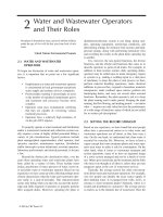
PHYSICAL - CHEMICAL TREATMENT OF WATER AND WASTEWATER - CHAPTER 7 pdf

Conventional Filtration

Filtration

is a unit operation of separating solids from fluids. Screening is defined
as a unit operation that separates materials into different sizes. Filtration also sepa-
rates materials into different “sizes,” so it is a form of screening, but filtration strictly
pertains to the separation of solids or particles and fluids such as in water. The
microstrainer discussed in Chapter 5 is a filter. In addition to the microstrainer, other
examples of this unit operation of filtration used in practice include the filtration of
water to produce drinking water in municipal and industrial water treatment plants,
filtration of secondary treated water to meet more stringent discharge requirements
in wastewater treatment plants, and dewatering of sludges to reduce their volume.
To differentiate it from Chapter 8, this chapter discusses only conventional
filtration. Chapter 8 uses membranes as the medium for filtration; thus, it is titled
advanced filtration.
Mathematical treatments involving the application of linear momentum to fil-
tration are discussed. Generally, these treatments center on two types of filters called
granular and cake-forming filters. These filters are explained in this chapter.

7.1 TYPES OF FILTERS

Figures 7.1 to 7.8 show examples of the various types of filters used in practice.
Filters may be classified as gravity, pressure, or vacuum filters.

Gravity filters

are
filters that rely on the pull of gravity to create a pressure differential to force the
water through the filter. On the other hand,

pressure

and

vacuum filters

are filters
that rely on applying some mechanical means to create the pressure differential
necessary to force the water through the filter.
The filtration medium may be made of perforated plates, septum of woven
materials, or of granular materials such as sand. Thus, according to the medium
used, filters may also be classified as

perforated plate, woven septum

, or

granular
filters

. The filtration medium of the microstrainer mentioned above is of perforated
plate. The filter media used in plate-and-frame presses and vacuum filters are of
woven materials. These units are discussed later.
Figures 7.1 and 7.2 show examples of gravity filters. The media for these filters
are granular. In both figures, the influents are introduced at the top, thereby utilizing
gravity to pull the water through the filter. Figure 7.1a is composed of two granular
filter media anthrafilt and silica sand; thus, it is called a

dual-media gravity filter

.
Figure 7.1a is a triple-media gravity filter, because it is composed of three media:
anthrafilt, silica sand, and garnet sand.
Generally, two types of granular gravity filters are used: slow-sand and rapid-
sand filters. In the main, these filters are differentiated by their rates of filtration.
7

TX249_frame_C07.fm Page 327 Friday, June 14, 2002 4:32 PM
© 2003 by A. P. Sincero and G. A. Sincero

328

Slow-sand filters

normally operate at a rate of 1.0 to 10 m

3

/d
.
m

2

, while

rapid-sand
filters

normally operate at a rate of 100 to 200 m

3

/d
.
m

2

. A section of a typical gravity
filter is shown in Figure 7.2.
The operation of a gravity filter is as follows. Referring to Figure 7.2, drain
valves C and E are closed and influent value A and effluent valve B are opened.
This allows the influent water to pass through valve A, into the filter and out of the
filter through valve B, after passing though the filter bed.
For effective operation of the filter, the voids between filter grains should serve
as tiny sedimentation basins. Thus, the water is not just allowed to swiftly pass
through the filter. For this to happen, the effluent valve is slightly closed so that the
level of water in the filter rises to the point indicated, enabling the formation of tiny
sedimentation basins in the pores of the filter. As this level is reached, influent and
effluent flows are balanced. It is also this level that causes a pressure differential
pushing the water through the bed. The filter operates at this pressure differential
until it is clogged and ready to be backwashed (in the case of the rapid-sand filter).
Backwashing will be discussed later in this chapter. In the case of the slow-sand filter,

FIGURE 7.1

(a) Dual-media filter; (b) triple-media filter.

FIGURE 7.2

A typical gravity filter.
Influent
Effluent Effluent
Influent
Intermix zone
Intermix zone
Coarse media
Coarse media
Finer media
Finer media
Finest media
Finest media
Underdrain
chamber
Underdrain
chamber
Anthrafilt
Silica
sand
Anthrafilt
Silica
sand
(a) (b)
Garnet
sand
Water level
during filtering
Water level

during
backwashing
Wash-water
trough
Bed expansion
limit
Sand
Influent
Drain
Effluent
A
C
B
Drain
Underdrain system
Wash water
500 mm
650 mm
600 mm
freeboard
500 mm
10 m
Wash-water
tank
h
Lb
l
2
E
Cornroller

TX249_frame_C07.fm Page 328 Friday, June 14, 2002 4:32 PM
© 2003 by A. P. Sincero and G. A. Sincero

329

it is not backwashed once it is clogged. Instead, the layer of dirt that collects on top
of the filter (called

smutzdecke

) is scraped for cleaning.
As shown, the construction of the bed is such that the layers are supported by an
underdrain mechanism. This support may simply be a perforated plate or septum.
The perforations allow the filtered water to pass through. The support may also be
made of blocks equipped with holes. The condition of the bed is such that the coarser
heavy grains are at the bottom. Thus, the size of these holes and the size of the
perforations of the septum must not allow the largest grains of the bed to pass through.
Figure 7.3 shows a cutaway view of a pressure filter. The construction of this
filter is very similar to that of the gravity filter. Take note of the underdrain construc-
tion in that the filtered water is passed through perforated pipes into the filtered water
outlet. As opposed to that of the gravity filter above, the filtered water does not fall
through a bottom and into the underdrain, because it had already been collected by
the perforated pipes. The coarse sand and graded gravel rest on the concrete subfill.
Using a pump or any means of increasing pressure, the raw water is introduced
to the unit through the raw water inlet. It passes through the bed and out into the
outlet. The unit is operated under pressure, so the filter media must be enclosed in
a shell. As the filter becomes clogged, it is cleaned by backwashing.
Thickened and digested sludges may be further reduced in volume by dewater-
ing. Various dewatering operations are used including vacuum filtration, centrifuga-

tion, pressure filtration, belt filters, and bed drying. In all these units, cakes are
formed. We therefore call these types of filtration

cake-forming filtration

or simply

cake filtration

. Figure 7.4a shows a sectional drawing of a plate-and-frame press. In

pressure filtration

, which operates in a cycle, the sludge is pumped through the unit,
forcing its way into

filter plates

. These plates are wrapped in

filter cloths

. With the
filter cloths wrapped over them, the plates are held in place by

filter frames

in
alternate plates-then-frames arrangement. This arrangement creates a cavity in the
frame between two adjacent plates.

FIGURE 7.3

Cutaway view of a pressure sand filter. (Courtesy of Permutit Co.)
Raw water
inlet
Filtered water
outlet
Weir
Drain
Sump
Manhole
Inlet baffle
Fine sand
Coarse sand
Graded gravel
Concrete subfill
Header lateral
strainer system
with expansible
strainer heads
Adjustable jack legs

TX249_frame_C07.fm Page 329 Friday, June 14, 2002 4:32 PM
© 2003 by A. P. Sincero and G. A. Sincero

330

Physical–Chemical Treatment of Water and Wastewater

FIGURE 7.4

(a) Sectional drawing of a plate-and-frame press (from T. Shriver and Co.); (b) an installation of a plate-and-frame
press (courtesy of Xingyuan Filtration Products, China).

TX249_frame_C07.fm Page 330 Friday, June 14, 2002 4:32 PM
© 2003 by A. P. Sincero and G. A. Sincero

331

Two channels are provided at the bottom and top of the assembly. The bottom
channel serves as a conduit for the introduction of the sludge into the press, while
the top channel serves as the conduit for collecting the filtrate. The bottom channel
has connections to the cavity formed between adjacent plates in the frame. The top
channel also has connections to small drainage paths provided in each of the plates.
These paths are where the filtrate passing through cloth are collected.
As the sludge is forced through the unit at the bottom part of the assembly (at
a pressure of 270 to 1,000 kPa), the filtrate passes through the filter cloth into the
drainage paths, leaving the solids on the cloth to accumulate in the cavities of the
frames. As determined by the cycle, the press is opened to remove the accumulated
and dewatered sludge. Figure 7.4b shows an installation of a plate-and-frame press unit.
Figures 7.5 to Figure 7.7 pertain to the use of rotary vacuum filters in vacuum
filtration. In

vacuum filtration

, a drum wrapped in filter cloth rotates slowly while
the lower portion is submerged in a sludge tank (Figure 7.7a). A vacuum applied in
the underside of the drum sucks the sludge onto the filter cloth, separating the filtrate
and, thus, dewatering the sludge.

A rotary vacuum filter is actually a drum over which the filtration medium is
wrapped. This medium is made of a woven material such as canvas. This medium is
also called a

filter cloth

. The drum is made of an outer shell and an inner shell.
These two shells form an annulus. The annulus is then divided into segments, which
are normally 30 cm in width and length extending across the entire length of the
drum. Figure 7.7a shows that there are twelve segments in this vacuum filter. The
outer shell has perforations or slots in it, as shown in the cutaway view of Figure
7.6. Thus, each segment has a direct connection to the filter cloth. The purpose of
the segments is to provide the means for sucking the sludge through the cloth while
it is still submerged in the tank.
Each of the segments are connected to the rotary valve through individual
pipings. As shown in Figure 7.7a, segments 1 to 5 are immersed in the sludge, while

FIGURE 7.5

A rotary vacuum filter in operation. (Courtesy of Oliver United Filters.)
Water
Wash liquor
Filtrate
Air
Blowback
Drum
Scraper or
“doctor knife”
Cake being
removed

Drive

TX249_frame_C07.fm Page 331 Friday, June 14, 2002 4:32 PM
© 2003 by A. P. Sincero and G. A. Sincero

segments 6 to 12 are not. Pipes

V

1

and

V

2

of the rotary valve are connected to an
external vacuum pump, as indicated in Figure 7.7b. The design of the rotary valve
is such that when segments are submerged in the sludge such as segments 1 to 5,
they are connected to pipe

V

1

through their individual connecting pipes. When
segments are not submerged such as segments 6 to 12, the design is also such that
these segments are connected to pipe

V

2

. This arrangement allows for suction of
sludge into the filter cloth over the segment when it is submerged (

V

1

) and drying
of the sludge when the segment is not submerged (

V

2

).
We can finalize the description of the operation of the vacuum filter this way.
As the segments that had been sucking sludge while they were still submerged in

FIGURE 7.6

Cutaway view of a rotary vacuum filter. (Courtesy of Swenson Evaporator Co.)

FIGURE 7.7

(a) Cross section of a rotary vacuum filter; (b) flow sheet for continuous vacuum
filtration.

Stationary
valve plate
Rotating wear plate
Port
Segments
Drum
Wash spray nozzles
Filter
medium
Agitator
arm
Scraper
Repulper
Tank
To separator
and vacuum
pump
Discharge
head
Valve

TX249_frame_C07.fm Page 332 Friday, June 14, 2002 4:32 PM
© 2003 by A. P. Sincero and G. A. Sincero

333

the tank emerge from the surface, their connections are immediately switched from

V

1

to

V

2

. The connection

V

2

completes the removal of removable water from the
sludges, whereupon the suction switches to sucking air into the segments promoting
the drying of the sludges. The “dry” sludge then goes to the scraper (also called

doctor blade

) and the sludge removed for further processing or disposal.
Figure 7.7b shows the fate of the filtrate as it is sucked from the filter cloth.
Two tanks called

vacuum receivers

are provided for the two types of filtrates: the
filtrate removed while the segments are still submerged in the tank and the residual
filtrate removed when the segments are already out of the tank. Vacuum receivers
are provided to trap the filtrate so that the filtrate will not flood the vacuum pump.

Also note the barometric seal. As shown, this is in parallel connection with the
suction vacuum of the filter. The vacuum pressure is normally set up to a value of
66 cm Hg below atmospheric. Any vacuum set for the filter will correspondingly
exert an equal vacuum to the barometric seal, on account of the parallel connection.
Hence, the length of this seal should be set equivalent to the maximum vacuum
expected to be utilized in the operation of the filter. If, for example, the filter is to
be operated at 51 cm,
where 13.6 is the mass density of mercury in gm/cc, and 1 is the density of water
also in gm/cc. Thus, from this result, the length of the barometric seal should be
6.94 m if the operational vacuum is 51 cm Hg. The design in Figure 7.7b shows the
length as 9.1 m.
Figure 7.8a shows another type of filter that operates similar to a rotary vacuum
filter in that it uses a vacuum pressure to suck sludge into the filter medium. This
type of filter is called a leaf filter. A

leaf filter

is a filter that operates by immersing
a component called a leaf into a bath of sludge or slurry and using a vacuum to suck
the sludge onto the leaf. An example of a leaf filter is shown in Figure 7.8b. As
indicated, it consists of two perforated plates parallel to each other, with a separator
screen providing the spacing between them. A filter is wrapped over the plate assem-
bly, just like in the plate-and-frame press. Each of the leaves are then attached into
a hub through a clamping ring. The hub has a drainage space that connects into the
central pipe through a small opening. As indicated in the cutaway view on the right
of Figure 7.8a, several of these leaves are attached to the central pipe. Each of the
leaves then has a connection to the central pipe through the small opening from the
drainage space. The central pipe collects all the filtrates coming from each of the leaves.
In operation, a vacuum pressure is applied to each of the leaves. The feed sludge
is then introduced at the feed inlet as indicated in the drawing. The sludge creates

a slurry pool inside the unit immersing the leaves. Through the action of the vacuum,
the sludge is sucked into the filter cloth. As the name implies, this is a rotary leaf
filter. The leaves are actually in the form of a disk. The disks are rotated, immersing
part of it in the slurry, just as part of the drum is immersed in the case of the rotary
vacuum filter. As the immersed part of the disks emerge from the slurry pool into
the air, the filtrate are continuously sucked by the vacuum resulting in a dry cake.
51 13.6()1()∆h
H
2
O
; ∆h
H
2
O
6.94 m==

TX249_frame_C07.fm Page 333 Friday, June 14, 2002 4:32 PM
© 2003 by A. P. Sincero and G. A. Sincero

334

Physical–Chemical Treatment of Water and Wastewater

FIGURE 7.8

A rotary leaf filter showing cutaway view at right end (courtesy of Swenson Evaporator Co.); (b) section of a leaf.
Feed inlet
(a)
Screw conveyor
Discharge connection

Hollow
shaft
Filtrate
outlet
Central pipe
Leaf
Leaf
Separator screen
Separator screen
Perforated plates
Perforated plates
Filter cloth
Filter cloth
Clamping rings
Clamping rings
Filter leaf hub
Filter leaf hub
Central pipe
(b)
Drainage
space
Drainage
space

TX249_frame_C07.fm Page 334 Friday, June 14, 2002 4:32 PM
© 2003 by A. P. Sincero and G. A. Sincero

335

A mechanism is provided for the cake to drop into a screw conveyor below for

continuous removal. This mechanism does not require opening of the case for removal
of the cake.
It may be noticed that some of the filters discussed are operated continuously and
some are not. For example, the rapid sand filter, the slow sand filter, the pressure filter,
and the rotary vacuum filter are all operated continuously. The plate-and-frame press
is operated as a batch. Thus, filters may also be classified as

continuous

and

discon-
tinuous

. Only the plate-and-frame press is discussed in this chapter as a representation
of the discontinuous type, but others are used, such as the shell-and-leaf filters and
the cartridge filters. The first operates in a mode that a leaf assembly is inserted into
a shell while operating and retracted out from the shell when it is time to remove the
cake. The second looks like a “cartridge” in outward appearance with the filter medium
inside it. The medium could be thin circular plates or disks stacked on top of each
other. The clearance between disks serves to filter out the solids.

7.2 MEDIUM SPECIFICATION FOR
GRANULAR FILTERS

The most important component of a granular filter is the medium. This medium
must be of the appropriate size. Small grain sizes tend to have higher head losses,
while large grain sizes, although producing comparatively smaller head losses, are
not as effective in filtering. The actual grain sizes are determined from what expe-
rience has found to be most effective. The actual medium is never uniform, so the

grain sizes are specified in terms of effective size and uniformity coefficient.

Effective
size

is defined as the size of sieve opening that passes the 10% finer of the medium
sample. The effective size is said to be the

10th percentile size



P

10

. The

uniformity
coefficient

is defined as the ratio of the size of the sieve opening that passes the 60%
finer of the medium sample (

P

60

) to the size of the sieve opening that passes the
10% finer of the medium sample. In other words, the uniformity coefficient is the

ratio of the

P

60

to the

P

10

. For slow-sand filters, the effective size ranges from 0.25
mm to 0.35 mm with uniformity coefficient ranging from 2 to 3. For rapid-sand
filters, the effective size ranges from 0.45 mm and higher with uniformity coefficient
ranging from 1.5 and lower.
Plot of a sieve analysis of a sample of run-of-bank sand is shown in Figure 7.9
by the segmented line labeled “stock sand ….” This sample may or may not meet
the required effective size and uniformity coefficient specifications. In order to
transform this sand into a usable sand, it must be given some treatment. The figure
shows the cumulative percentages (represented by the “normal probability scale” on
the ordinate) as a function of the increasing size of the sand (represented by the
“size of separation” on the abscissa).
Let

p

1

be the percentage of the sample stock sand that is smaller than or equal

to the desired

P

10

of the final filter sand, and

p

2

be the percentage of the sample
stock sand that is smaller than or equal to the desired

P

60

of the final filter sand.
Since the percentage difference of the

P

60

and

P

10

represents half of the final filter
sand,

p

2



−



p

1

must represent half of the stock sand that is transformed into the final

TX249_frame_C07.fm Page 335 Friday, June 14, 2002 4:32 PM
© 2003 by A. P. Sincero and G. A. Sincero

filter sand. Letting

p

3

be the percentage of the stock sand that is transformed into
the final filter sand,

p

3



=

2(

p

2



−



p

1

) (7.1)
Of this

p

3

, by definition, 10% must be the

P

10

of the final sand. Therefore, if

p

4

is the percentage of the stock sand that is too fine to be usable,

p

4



=



p

1



−

0.1

p

3



=



p

1



−

0.1(2)(

p

2



−



p

1

) (7.2)
The plot in the figure shows an increasing percentage as the size of separation
increases, so the sum of p
4
and p
3
must represent the percentage of the sample stock
sand above which the sand is too coarse to be usable. Letting p
5
be this percentage,
p
5
= p
4
+ p
3
(7.3)
Now, to convert a run-of-bank stock sand into a usable sand, an experimental

curve such as Figure 7.9 is entered to determine the size of separation corresponding
to p
4
and p
5
. Having determined these sizes, the stock sand is washed in a sand
washer that rejects the unwanted sand. The washer is essentially an upflow settling
FIGURE 7.9 Sieve analysis of run-of-bank sand.
99
98
95
90
80
70
60
50
40
30
20
10
5
2
1
0.5
0.2
0.1
Normal probability scale
10
-2 2 3 4 5 6 7 8 9
10

-1 2 3 4 5 6 7 8 9 1
Size of separation (cm)
Filter sand (wanted)
E
= 5 × 10
-2
cm,
U
= 1.5
Stock sand (available)
E
= 3 × 10
-2
cm,
U
= 2.8
Analysis of stock sand
Site of
separation
cm × 10
-2
Cumulative
weight
%
1.05
1.49
2.10
2.97
4.2
5.9

8.4
11.9
16.8
23.8
33.6
0.2
0.9
4.0
9.9
21.8
39.4
59.8
74.4
93.3
96.8
100.0
TX249_frame_C07.fm Page 336 Friday, June 14, 2002 4:32 PM
© 2003 by A. P. Sincero and G. A. Sincero
tank. By varying the upflow velocity of the water in the washer, the sand particles
introduced into the tank are separated by virtue of the difference of their settling
velocities. The lighter ones are carried into the effluent while the heavier ones remain.
The straight line in the figure represents the size distribution in the final filter sand
when the p
4
and fractions greater than p
5
have been removed.
Example 7.1 If the effective size and uniformity coefficient of a proposed filter
is to be 5(10
−2

) cm and 1.5, respectively, perform a sieve analysis to transform the
run-of-bank sand of Figure 7.9 into a usable sand.
Solution: From Figure 7.9, for a size of separation of 5(10
−2
) cm, the percent
p
1
is 30. Also, the P
60
size is 5(10
−2
)(1.5) = 7.5(10
−2
) cm. From the figure, the percent
p
2
corresponding to the P
60
size of the final sand is 53.
Therefore, the sand washer must be operated so that the p
4
sizes of 4.5(10
−2
) cm and
smaller and the p
5
sizes of 1.1(10
−1
) cm and greater are rejected. Ans
7.3 LINEAR MOMENTUM EQUATION

APPLIED TO FILTERS
The motion of water through a filter bed is just like the motion of water through
parallel pipes. While the motion through the pipes is straightforward, however, the
motion in the filter bed is tortuous. Figure 7.10 shows a cylinder or pipe of fluid
and bed material. Inside this pipe is an element composed of fluid and bed material
being isolated with length dl and interstitial area A and subjected to forces as shown.
(We use the term interstitial area here because the bed is actually composed of grains.
The fluid is in the interstitial spaces between grains.) The equation of linear momen-
tum may be applied on the water flow in the downward direction of this element, thus,
(7.4)
where ∑F
z
is the net unbalanced force in the downward z direction; p is the hydro-
static pressure; A is the interstitial cross-sectional area of the cylindrical element of
fluid; F
g
is the weight of the fluid in the element; F
sh
is the shear force acting on
the fluid along the surface areas of the grains; is the volume of element of space;
dl is the differential length of the element, l being any distance from some origin;
A
s
is the surface area of all the grains; k is a factor that converts A
s
into an area such
that kA
s
dl =
η

d ;
η
is the porosity of the bed; a
z
is the acceleration of the fluid
p
3
2 p
2
p
1
–()253 30–()46%===
p
4
p
1
0.1 p
3
()– 30 0.1 46()–==
25.4%; from the figure, the corresponding size of separation=
4.5 10
2–
() cm=
p
5
46 25.4+ 71.4%; corresponding size of separation 1.1 10
1–
() cm== =
F
z

∑
pA p dp+()A– F
g
F
sh
–+
ρη
dV a
z
=
ρη
dV
dv
dt

ρ
kA
s
dl
dv
dt

===
F
z
∑
dpA– F
g
F
sh

–+
ρ
kA
s
dl
dv
dt

==
dV
V
TX249_frame_C07.fm Page 337 Friday, June 14, 2002 4:32 PM
© 2003 by A. P. Sincero and G. A. Sincero
element in the downward z direction;
ρ
is the fluid mass density; v is the component
fluid element velocity in the z direction; and t is the time. Since the fluid is in the
interstitial spaces, d needs to be multiplied by the porosity to get the fluid volume.
The law of inertia states that a body at rest will remain at rest and a body in
uniform motion will remain in this uniform motion unless acted upon by an unbal-
anced force. ∑F
z
=
ρ
kA
s
dl(dv/dt) is this unbalanced force that breaks this inertia;
thus, it is called the inertia force. By the chain rule, (dv/dt) = (dv/dl)(dl/dt) = v(dv/dl).
Thus,
ρ

kA
s
dl(dv/dt) =
ρ
kA
s
dlv(dv/dl) =
ρ
kA
s
vdv. Let be some characteristic aver-
age pipe velocity.
The velocity through the pipe could vary from the entrance to the exit. represents
the average of these varying values; hence, it is a constant. Note that all the velocities
referred to here are interstitial velocities, the true velocities of the fluid as it travels
through the pores.
Now, let v
∗
= v/ . Hence, dv
∗
= dv/ , and
ρ
kA
s
vdv =
ρ
kA
s
( v
∗

) dv
∗
=
ρ
kA
s
2
v
∗
dv
∗
. Thus, the inertial force ∑F
z
=
ρ
kA
s
vdv, in effect, is proportional to
ρ
A
s
2
;
the presence of v
∗
dv
∗
does not nullify this fact. Calling the proportionality constant as
K
i

,
(7.5)
In light of this new information, Equation (7.4) may now be solved for −dpA,
which is −∆pA when applied to the whole length of pipe, producing
−∆pA = K
i
ρ
A
s
+ F
sh
− F
g
(7.6)
To address F
sh
, let us recall the Hagen–Poiseuille equation from fluid mechanics.
FIGURE 7.10 Free-body diagram of a cylinder (pipe) of fluid and bed material.
Cylinder of fluid and bed
V
V
V
V V V
V
V V
F
z
∑
K
i

ρ
A
s
V
2
=
V
2
TX249_frame_C07.fm Page 338 Friday, June 14, 2002 4:32 PM
© 2003 by A. P. Sincero and G. A. Sincero
This is written as
(7.7)
−∆p
s
is the pressure drop due to shear forces;
µ
is the absolute viscosity of the fluid;
l is the length of pipe; and D is the diameter of pipe. In a bed of grains, the cross-
sectional area of flow is so small that the boundary layer created as the flow passes
around one grain overlaps with the boundary layer formed in a neighboring grain.
Because boundary layer flow is, by nature, laminar, flows through beds of grain is
laminar and Equation (7.7) applies.
F
sh
is a shear force acting on the fluid along the surface areas of the grains. The
shear stress is this −∆p
s
; thus, F
sh
= −∆p

s
A
s
. From this relationship and the equation
for ∆p
s
, we glean that the F
sh
is directly proportional to
µ
, , and l and inversely
proportional to the square of D. The granular filter is not really a pipe, so we replace
D by the hydraulic radius r
H
. With D expressed in terms of r
H
, the equation becomes
general. In other words, it can be used for any shape, because r
H
is simply defined
as the area of flow divided by the wetted perimeter. The proportionality relation is
Dimensionally, l and may be canceled leaving only r
H
in the
denominator. Calling the overall proportionality constant as K
s
, F
sh
= K
s

(
µ
A
s
/r
H
);
and Equation (7.6) becomes
(7.8)
To address F
g
, it must be noted that for a given filter installation it is a constant.
It is a constant, so its effect when the variables are varied is also a constant. This
effect will be subsumed into the values of K
i
and K
s
. We can therefore safely remove
F
g
from the equation and write simply
(7.9)
This is the general linear momentum equation as applied to any filter.
7.4 HEAD LOSSES IN GRAIN FILTERS
Head losses in granular filters may be divided into two categories: head loss in clean
filters and head loss due to the deposited materials. We will now discuss the first
category.
7.4.1 CLEAN-FILTER HEAD LOSS
To derive the clean-filter head loss, we continue with Equation (7.9) by expressing
A

s
, r
H
, and in terms of their equivalent expressions. Let s
p
be the surface area of
a particle and let N be the number of grains in the bed. Thus, A
s
= Ns
p
. Let S
o
be
the empty bed or superficial area of the bed. With the porosity
η
and length l, the
∆p
s
–
32
µ
lV
D
2

=
V
F
sh
∞

µ
lV A
s
/r
H
2
. r
H
2
V
∆pA– K
i
ρ
A
s
V
2
K
s
µ
VA
s
r
H
F
g
–+=
∆pA– K
i
ρ

A
s
V
2
K
s
µ
VA
s
r
H

+ A
s
K
i
ρ
V
2
K
s
µ
V
r
H

+


==

V
TX249_frame_C07.fm Page 339 Friday, June 14, 2002 4:32 PM
© 2003 by A. P. Sincero and G. A. Sincero
volume of the bed grains is S
o
l(1 −
η
). Letting v
p
represent the volume of a grain,
N is also calculated as Thus, A
s
is
(7.10)
Consider first that the grains are spherical. For spherical particles, v
p
=
π
d
3
/6
and s
p
=
π
d
2
, where d is the diameter of the particle. Therefore, s
p
/v

p
= 6/d. Substi-
tuting in Equations (7.10),
(7.11)
The expression area of flow divided by the wetted perimeter for the hydraulic
radius is the same as volume of flow divided by the wetted area, that is,
(7.12)
With N as the number of medium grains in the filter each of volume v
p
, the
volume of the filter is Nv
p
/(1 −
η
). Therefore, the volume of flow is
η
[Nv
p
/(1 −
η
)]
and the hydraulic radius becomes
(7.13)
The velocity is the interstitial velocity of the fluid through the pores of the
bed. Compared to the superficial velocity , it is faster due to the effect of the
porosity
η
. (The cross-sectional area of flow is much constricted, hence, the velocity
is much faster.) In terms of
η

and ,
(7.14)
Substituting Eqs. (7.11), (7.13), and (7.14) in Equation (7.9) and simplifying
produces
(7.15)
(7.16)
where Re is the Reynolds number defined as . Ergun (1952) correlating a
mass of experimental data showed that 6K
i
= 1.75 and 36K
s
= 150. Thus,
(7.17)
S
o
l 1
η
–()/v
p
.
A
s
s
p
v
p

S
o
l 1

η
–()=
A
s
6
d

S
o
l 1
η
–()=
r
H
volume of flow
wetted area

=
r
H
η
N v
p
1
η
–()

Ns
p

η
1
η
–



v
p
s
p



η
1
η
–



d
6

== =
V
V
s
V
s

V
V
s
η

=
∆pA–
S
o
l 1
η
–()V
s
2
ρ
d
η
2

6K
i
36K
s
1
η
–()
dV
s
ρ
/

µ

+=
∆pA–
S
o
l 1
η
–()V
s
2
ρ
d
η
2

6K
i
36K
s
1
η
–()
Re

+=
dV
s
ρ
/

µ
∆pA–
S
o
l 1
η
–()V
s
2
ρ
d
η
2

= 1.75
150 1
η
–()
Re

+
S
o
l 1
η
–()V
s
2
ρ
d

η
2

f
p
=
TX249_frame_C07.fm Page 340 Friday, June 14, 2002 4:32 PM
© 2003 by A. P. Sincero and G. A. Sincero
where
f
p
= 1.75 + a form of friction factor. (7.18)
A is equal to S
o
η
. Substituting in Equation (7.17), the pressure drop across the
filter is finally given as
(7.19)
γ
is the specific weight of the fluid. In terms of the equivalent height of fluid, we
use the relationship −∆p =
γ
h
L
, where h
L
is the head loss across the filter. Thus,
(7.20)
The equations treated above all refer to the diameter of spherical particles; yet
in practice, not all particles are spherical. To use the above equations for these

situations, the sieve diameter must be converted to its equivalent spherical diameter.
In Chapter 5, the relationship was given as d = (6/
π
)
1/3
β
1/3
d
p
, where
β
is the shape
factor and d
p
is the sieve diameter.
Equation (7.20) has been derived for a bed of uniform grain sizes. In some types
of filtration plants such as those using rapid sand filters, however, the bed is back-
washed every so often. This means that after backwashing, the grain particles are
allowed to settle; the grain deposits on the bed, layer by layer, are of different sieve
diameters. The bed is said to be stratified. To find the head loss across a stratified
medium, Equation (7.20) is applied layer by layer, each layer being converted to
one single, average diameter. The head losses across each layer are then summed
to produce the head loss across the bed as shown next.
(7.21)
where the index i refers to the ith layer. If x
i
is the fraction of the d
i
particles in the
ith layer, then l

i
equals x
i
l. Assuming the porosity
η
is the same throughout the bed,
the equation becomes
(7.22)
Note, again, that d
i
is for a spherical particle. For nonspherical particles, the sieve
diameter d
p
must be converted into its equivalent spherical particle by the equation
mentioned in a previous paragraph.
150 1
η
–()
Re

,
∆p– f
p
2
γ
l 1 n–()
n
3
d

V
s
2
2g

=
h
L
f
p
2l 1 n–()
n
3
d

V
s
2
2g

=
h
L
f
pi
2l
i
1 n–()
n
3

d
i

V
s
2
2g

∑
=
h
L
f
pi
2x
i
l 1 n–()
n
3
d
i

V
s
2
2g

∑
2l 1 n–()
n

3

V
s
2
2g

f
pi
x
i
d
i

∑
==
TX249_frame_C07.fm Page 341 Friday, June 14, 2002 4:32 PM
© 2003 by A. P. Sincero and G. A. Sincero
Example 7.2 A sharp filter sand has the sieve analysis shown below. The poros-
ity of the unstratified bed is 0.39, and that of the stratified bed is 0.42. The lowest
temperature anticipated of the water to be filtered is 4°C. Find the head loss if the
sand is to be used in (a) a slow-sand filter 76 cm deep operated at 9.33 m
3
/m
2
⋅ d and
(b) a rapid-sand filter 76 cm deep operated at 117 m
3
/m
2

⋅ d.
Solution:
Therefore,
Sieve No.
Average Size
(mm) x
i
14–20 1.0 0.01
20–28 0.70 0.05
28–32 0.54 0.15
32–35 0.46 0.18
35–42 0.38 0.18
42–48 0.32 0.20
48–60 0.27 0.15
60–65 0.23 0.07
65–100 0.18 0.01
(a) h
L
f
p
2l 1 n–()
n
3
d

V
s
2
2g

=
d
pave
1 0.01()0.7 0.05()0.54 0.15()0.46 0.18()0.38 0.18()++ + +=
0.32 0.20()0.27 0.15()0.23 0.07()0.18 0.01()++++
0.40 mm=
9.33m
3
/m
2
d⋅ 1.08 10
4–
() m/s=
f
p
1.75
150 1
η
–()
Re
+=
Re dV
s
ρ
/
µ
=
d 1.24
β
0.333

d
p
β
0.77==
d 1.24 0.77
0.333
()0.40()10
3–
()0.45 10
3–
() m==
µ
15 10
4–
() kg/m s⋅ at 20°C=
Re
0.45 10
3–
()1.08()10
4–
()1000()
15 10
4–
()

0.0324==
f
p
1.75 150
1 0.39–()

0.0324

+ 2,825.82==
h
L
2,825.82
2 0.76()1 0.39–()1.08 10
4–
()[]
2
0.39
3
0.45()10
3–
()2()9.81()

=
3.056 10
5–
()
5.24 10
4–
()

0.058 m Ans==
TX249_frame_C07.fm Page 342 Friday, June 14, 2002 4:32 PM
© 2003 by A. P. Sincero and G. A. Sincero
7.4.2 HEAD LOSSES DUE TO DEPOSITED MATERIALS
The head loss expressions derived above pertain to head losses of clean filter beds.
In actual operations, however, head loss is also a function of the amount of materials

deposited in the pores of the filter. Letting q represent the deposited materials per
unit volume of bed, the corresponding head loss h
d
as a result of this deposited
materials may be modeled as
h
d
= a(q)
b
(7.23)
where a and b are constants. Taking logarithms,
ln h
d
= ln a + bln q (7.24)
This equation shows that plotting lnh
d
against lnq will produce a straight line. By
performing experiments, Tchobanoglous and Eliassen (1970) showed this statement
to be correct.
Sieve No. Avg. Size (mm) x
i
f
i
14–20 1.0 0.01 86.75 763.28
20–28 0.70 0.05 123.18 7741.44
28–32 0.54 0.15 159.16 38,899.02
32–35 0.46 0.18 186.53 64,221.10
35–42 0.38 0.18 225.43 93,955.69
42–48 0.32 0.20 267.34 147,033.13
48–60 0.27 0.15 316.56 154,740.68

60–65 0.23 0.07 371.32 99,432.26
65–100 0.18 0.01 473.97 23,168.33
∑ = 629,977.93
(b) 117 m
3
/m
2
d⋅ 0.00135 m/s=
h
L
2l 1 n–()
n
3

V
s
2
2g

f
pi
x
i
d
i

∑
=
Re
i

d
i
0.00135()1000()
15 10
4–
()
=
1.24 0.77()
0.333
d
pi
0.00135()1000()
15 10
4–
()
1022.98d
pi
==
f
p
1.75 150
1 0.42–()
1022.98d
pi

+
0.85
d
pi
1.75+==

f
pi
x
i
d
i

f
p
x
i
1.24(0.77
0.333
)d
pi

==
==
h
L
2l 1 n–()
n
3

V
s
2
2g

f

pi
x
i
d
i

∑
2 0.76()1 0.42–()0.00135
2
()
0.42
3
2()9.81()

629,977.93()==
0.696 m Ans=
TX249_frame_C07.fm Page 343 Friday, June 14, 2002 4:32 PM
© 2003 by A. P. Sincero and G. A. Sincero
Letting h
Lo
represent the clean-bed head loss, the total head loss of the filter bed
h
L
is then
h
L
= h
Lo
+ h
d

= h
Lo
+ ∑a(q
i
)
b
(7.25)
where h
d
is the head loss over the several layers of grains in the bed due to the
deposited materials.
Now, let us determine the expression for q. This expression can be readily derived
from a material balance using the Reynolds transport theorem. This theorem is
derived in any good book on fluid mechanics and will not be derived here. The
derivation is, however, discussed in the chapter titled “Background Chemistry and
Fluid Mechanics.” It is important that the reader acquire a good grasp of this theorem
as it is very fundamental in understanding the differential form of the material
balance equation. This theorem states that the total derivative of a dependent variable
is equal to the partial derivative of the variable plus its convective derivative. In
terms of the deposition of the material q onto the filter bed, the total derivative is
(7.26)
is the volume of the control volume. The partial derivative (also called local deriv-
ative) is
(7.27)
and the convective derivative is
(7.28)
The symbol ͛
A
means that the integration is to be done around the surface area of
the volume. The vector is a unit vector on the surface and normal to it and the

vector is the velocity vector through the surface for the flow into the filter. Now,
substituting these equations into the statement of the Reynolds theorem, we obtain
(7.29)
In the previous equation, the total derivative is also called Lagrangian derivative,
material derivative, substantive derivative, or comoving derivative. The combination
of the partial derivative and the convective derivative is also called the Eulerian
derivative. Again, it is very important that this equation be thoroughly understood.
It is to be noted that in the environmental engineering literature, many authors
confuse the difference between the total derivative and the partial derivative. Some
authors use the partial derivative instead of the total derivative and vise versa. As
shown by the previous equation, there is a big difference between the total derivative
and the partial derivative. If this difference is not carefully observed, any equation
written that uses one derivative instead of the other is conceptually wrong; this
total derivative
d
dt

qVd
V
∫


=
V
partial derivative
∂
∂
t

qVd

V
∫


=
convective derivative cv
A
∫
°
n
ˆ
η
dA⋅=
n
ˆ
v
d
dt

qVd
V
∫


∂
∂
t

qVd
V

∫


cv
A
∫
°
n
ˆ
η
dA⋅+=
TX249_frame_C07.fm Page 344 Friday, June 14, 2002 4:32 PM
© 2003 by A. P. Sincero and G. A. Sincero
confusion can be seen very often in the environmental engineering literature. Thus,
caution in reading the literarture should be exercised.
Over a differential length dl and cross-sectional area A of bed,
(7.30)
where and Q = flow, a constant through the bed. (The minus sign of
results from the fact that at the inlet the unit normal vector is in opposite direction
to that of the velocity vector .) Therefore,
(7.31)
V
s
is the superficial velocity of flow in the bed.
Also, over the same differential length dl and cross-sectional area S
o
of bed,
(7.32)
d in the second term has been taken out of the parentheses, because it is arbitrary
and therefore independent of t.

Substituting Eqs. (7.31) and (7.32) in Equation (7.29),
(7.33)
(Since the solids are conservative substances, the total derivative is equal to zero.)
Dividing out S
o
dl and rearranging,
(7.34)
The numerical counterpart of Equation (7.34), using n as the index for time and
m as the index for distance, is
(7.35)
for the first time-step. Solving for q
n+1
,
(7.36)
The equation for the second time-step is
(7.37)
cv n
ˆ
η
dA⋅
A
∫
°
−m˙ m˙
∂
m˙
∂
l

dl+



+
∂
m˙
∂
l

dl==
m˙ cQ= m˙
n
ˆ
v
cv n
ˆ
η
dA⋅
A
∫
°
∂
m˙
∂
l

dl Q
∂
c
∂
l

dl V
s
S
o
∂
c
∂
l

dl== =
∂
∫
V
qdV
∂
t

∂
qdV()
∂
t

∂
q
∂
t

dV
∂

q
∂
t

S
o
dl===
V
∂
q
∂
t

S
o
dl V
s
S
o
∂
c
∂
l

dl+ 0=
∂
q
∂
t

V
s
∂
c
∂
l

–=
q
n+1,m
q
n,m
–
∆t
V
s
c
n,m+1
c
n,m
–
∆l

–=
q
n+1,m
q
n,m
∆tV
s

∆l

c
n,m−1
c
n,m
–()– q
n,m
∆tV
s
∆c
n
∆l

–==
q
n+2,m
q
n+1,m
∆tV
s
∆c
n+1
∆l

– q
n,m
∆tV
s
∆c

n
∆l

– ∆tV
s
∆c
n+1
∆l

–==
TX249_frame_C07.fm Page 345 Friday, June 14, 2002 4:32 PM
© 2003 by A. P. Sincero and G. A. Sincero
Over a length ∆l, the gradients ∆c/∆l varies negligibly from time step to time
step. Thus, ∆c
n
/∆l = ∆c
n+1
/∆l = ∆c
n+2
/∆l and so on. Equation (7.37) may then be
written as
(7.38)
For the kth time step, the numerical equation becomes
(7.39)
But the number of time steps k is t/∆t. Therefore, the numerical equation is simply
(7.40)
q
n+k,m
is actually simply q at the end of filtration. Also, q
n,m

at the beginning of the
filtration run is zero. Because the effect of the deposited materials has to start
from a clean filter bed, q
n,m
may be removed from the equation. The final equation
becomes
(7.41)
The nature and sizes of particles introduced to the filter will vary depending
upon how they are produced. Thus, the influent to a filter coming from a softening
plant is different than the influent coming from a coagulated surface water. Also,
the influent coming from a secondary-treated effluent is different than that of any
of the drinking water treatment influent. For these reasons, in order to use the
previous equations for determining head losses, a pilot plant study should be con-
ducted for a given type of influent.
Determination of constants a and b. As noted before, h
d
plots a straight line
in logarithmic form with q. This means that only two data points are needed in order
to determine the constants a and b. Let the data points be (h
d1
, q
1
) and (h
d2
, q
2
). The
two equations for h that can be used to solve for the constants are then
h
d1

= a(q
1
)
b
(7.42)
h
d2
= a(q
2
)
b
(7.43)
q
n+2,m
q
n,m
2∆tV
s
∆c
∆l

–=
q
n+k,m
q
n,m
k∆tV
s
∆c
∆l

–=
q
n+k,m
q
n,m
tV
s
∆c
∆l

–=
qtV
s
∆c
∆l

–=
TX249_frame_C07.fm Page 346 Friday, June 14, 2002 4:32 PM
© 2003 by A. P. Sincero and G. A. Sincero
These equations may be solved simultaneously for a and b producing
(7.44)
(7.45)
If the number of data points is more than two, the data may be grouped to form
two data points. Using i as the index for the first group and j as the index for the second,
(7.46)
(7.47)
s
i
and s

j
refer to the total number of member elements in the respective groups. The
previous equations are actually calculating the means of the two groups.
Example 7.3 In order to determine the values of a and b of Equation (7.23),
experiments were performed on uniform sands and anthracite media yielding the fol-
lowing results below. Calculate the a’s and b’s corresponding to the respective diameters.
Dia., (mm) q (mg/cm
3
) h
d
(m)
Uniform Sand
0.5 1.08 0.06
0.5 7.2 4.0
0.7 1.6 0.06
0.7 11.0 4.0
1.0 2.6 0.06
1.0 17.0 4.0
Uniform Anthracite
1.0 6.2 0.06
1.0 43 4.0
1.6 8.1 0.06
1.6 58 4.0
2.0 9.2 0.06
2.0 68 4.0
b
h
d2
h
d1

ln
q
2
q
1

ln

=
a
h
d1
q
1
()
h
d2
h
d1
ln


q
2
q
1
ln



=
h
d1
∑
s
i
h
di
s
i

; q
1
∑
s
i
q
i
s
i

==
h
d2
∑
s
j
h
dj

s
j

; q
2
∑
s
j
q
j
s
j

==
TX249_frame_C07.fm Page 347 Friday, June 14, 2002 4:32 PM
© 2003 by A. P. Sincero and G. A. Sincero
Solution: Uniform sand, diameter = 0.5 mm:
Uniform sand, diameter = 0.7 mm:
Similar procedures are applied to the rest of the data. The following is the final
tabulation of the answers:
From the results of this example, the equations below with the values of b averaged
are obtained.
h
d
= 0.051(q)
2.22
for uniform sand, 0.5 mm diameter
h
d
= 0.022(q)

2.22
for uniform sand, 0.7 mm diameter
h
d
= 0.0133(q)
2.22
for uniform sand, 1.0 mm diameter
h
d
= 0.00114(q)
2.10
for uniform anthracite, 1.0 mm diameter
h
d
= 0.00069(q)
2.10
for uniform anthracite, 1.6 mm diameter
h
d
= 0.00057(q)
2.10
for uniform anthracite, 2.0 mm diameter
The h’s and q’s in the previous equations are in meters and mg/cm
3
, respectively.
Also, the head losses for diameters not included in the equations may be interpolated
or extrapolated from the results obtained from the equations.
Diameter (mm) ab
Sand 0.5 0.051 2.24
0.7 0.0216 2.18

1.0 0.0133 2.24
Anthracite 1.0 0.00114 2.17
1.6 0.00069 2.13
2.0 0.00057 2.01
a
h
d1
q
1
()
ln
h
d2
h
d1



ln
q
2
q
1




0.06
1.08()
ln

4.0
0.06



ln
7.2
1.08




0.051 Ans== =
b
ln
h
d2
h
d 1

ln
q
2
q
1


ln
4.0
0.06

ln
7.2
1.08


2.21 Ans== =
a
h
d1
q
1
()
ln
h
d2
h
d1



ln
q
2
q
1




0.06
1.60()
ln
4.0
0.06



ln
11
1.60




0.0216 Ans== =
b
ln
h
d2
h
d1

ln
q
2
q
1

ln
4.0
0.06

ln
11
1.60


2.18 Ans== =
TX249_frame_C07.fm Page 348 Friday, June 14, 2002 4:32 PM
© 2003 by A. P. Sincero and G. A. Sincero
Example 7.4 The amount of suspended solids removed in a uniform anthracite
medium, 1.8 mm in diameter is 40 mg/cm
3
. Determine the head loss due to suspended
solids.
Solution:
Interpolating, let x be the head loss corresponding to the 1.8-mm-diameter media.
Example 7.5 According to a modeling evaluation of the Pine Hill Run sewage
discharge permit, a secondary-treated effluent of 20 mg/L can no longer be allowed
into Pine Hill Run, an estuary tributary to the Cheseapeake Bay. To meet the new,
more stringent discharge requirement, the town decided to investigate filtering the
effluent. A pilot study was conducted using a dual-media filter composed of anthracite
as the upper 30-cm part and sand as the next lower 30-cm part of the filter. The results
are shown in the following table, where c
o
is the concentration of solids at the influent
and c is the concentration of solids in the water in the pores of the filter.
If the respective average sizes of the anthracite and sand layers are 1.6 mm and

0.5 mm, what is the length of the filter run to a terminal head loss of 3 m at a
filtration rate of 200 L/m
2
⋅ min? Assume the clean water head loss is 0.793 m. Note:
Terminal head loss is the loss when the filter is about to be cleaned.
Q
(L/m
2
⋅ min)
Depth,
cm c/c
o
Medium
Q
(L/m
2
⋅ min)
Depth,
(cm) c/c
o
Medium
80 0 1.0 Anthracite 80 8 0.32 Anthracite
80 16 0.27 Anthracite 80 24 0.24 Anthracite
80 30 0.23 Anthracite 80 40 0.20 Sand
80 48 0.20 Sand 80 56 0.20 Sand
160 0 1.0 Anthracite 160 8 0.46 Anthracite
160 16 0.30 Anthracite 160 24 0.27 Anthracite
160 30 0.25 Anthracite 160 40 0.22 Sand
160 48 0.22 Sand 160 56 0.22 Sand
240 0 1.0 Anthracite 240 8 0.59 Anthracite

240 16 0.39 Anthracite 240 24 0.30 Anthracite
240 30 0.27 Anthracite 240 40 0.23 Sand
240 48 0.23 Sand 240 56 0.23 Sand
h
d
0.00069 q()
2.10
for uniform anthracite, 1.6 mm diameter meter=
0.00069 40()
2.10
1.59 m==
h
d
0.00057 q()
2.10
for uniform anthracite, 2.0 mm diameter=
0.00057 40()
2.10
1.32 m==
1.59 x–
1.59 1.32–

1.6 1.8–
1.6 2.0–

; x 1.46 m Ans==
TX249_frame_C07.fm Page 349 Friday, June 14, 2002 4:32 PM
© 2003 by A. P. Sincero and G. A. Sincero
Solution: Because 200 L/m
2

⋅ min is between 160 and 240 L/m
2
⋅ min, only
the data for these two flows will be analyzed. The length of the filter run for the
200 L/m
2
⋅ min flow will be interpolated between the lengths of filter run of the 160
and the 240 flows.
Column 1 = given
Column 2 = 20 (column 1)
Column 3 = c
i,m+1
− c
i,m
; for example, −10.8 = 9.2 − 20
Therefore,
Filtration Rate (L/cm
2
⋅ min)
160 240
Depth
(cm)
(1) (2) (3) (4) (5) (6)
c/c
o
c (mg/L) ∆c
i
c/c
o
c (mg/L) ∆c

i
0 1 20. — 1 20 —
8 0.46 9.2 −10.8 0.59 11.8 −8.2
16 0.30 6.0 −3.2 0.39 7.8 −4.0
24 0.27 5.4 −0.6 0.3 6.0 −1.8
30 0.25 5.0 −0.4 0.27 5.4 −0.6
40 0.22 4.4 −0.6 0.23 4.6 −0.8
48 0.22 4.4 0 0.23 4.6 0
56 0.22 4.4 0 0.23 4.6 0
qtV
s
∆c
∆l

–=
160 L/m
2
min⋅
160 1000() cm
3
100
2
cm
2
min⋅

16 cm/min==
240 L/m
2
min⋅

240 1000() cm
3
100
2
cm
2
min⋅

24 cm/min==
1 mg/L
1 mg
1000 cm
3

10
3–
mg/cm
3
==
∆c
i
mg/L ∆c
i
10
3–
() mg/cm
3
=
qtV
s

∆c
∆l

– tV
s
10
3–
()
∆c
i,n
∆ᐉ
i

mg/cm
3
–==
h
d
0.00069 q()
2.10
for uniform anthracite, 1.6 mm diameter=
h
d
0.051 q()
2.22
for uniform sand, 0.5 mm diameter=
TX249_frame_C07.fm Page 350 Friday, June 14, 2002 4:32 PM
© 2003 by A. P. Sincero and G. A. Sincero
The terminal head loss of 3 m is composed of the clean water head loss of
0.793 m and the head loss due to deposited solids of h

s
Run Length (min)
For the 160 L//
//
cm
2
⋅⋅
⋅⋅
min 600 900 1200
Depth
(cm)
∆∆
∆∆
c
i

(mg/L)
∆∆
∆∆
l
i

(cm) ∆∆
∆∆
c
i
/∆∆
∆∆
ᐉ
i

q
i

(mg/cm
3
)
h
di

(m
3
)
q
i

(mg/cm
3
)
h
di

(m
3
)
q
i

(mg/cm
3
)

h
di

(m
3
)
0——— ——————
8 −10.8 8 −1.35 12.96 0.15 19.44 0.35 25.92 0.64
16 −3.2 8 −0.4 3.84 0.01 5.76 0.027 7.68 0.05
24 −0.6 8 −0.075 0.72 0.00 1.08 0.00 1.44 0.001
30 −0.4 6 −0.07 0.64 0.00 0.96 0.00 1.28 0.001
40 −0.6 10 −0.06 0.576 0.015 0.864 0.037 1.15 0.07
480—— ——————
∑h
i
= 0.175 ∑h
i
= 0.414 ∑h
i
= 0.762
Run Length (min)
For the 240 L/cm
2
⋅⋅
⋅⋅
min 1500 2100
Depth
(cm)
∆∆
∆∆

c
i

(mg/L) ∆∆
∆∆
l
i
(cm) ∆∆
∆∆
c
i
//
//
∆∆
∆∆
l
i
q
i

(mg/cm
3
) h
di
(m
3
)
q
i

(mg/cm
3
) h
di
(m
3
)
0———————
8 −8.2 8 −1.03 37.08 1.36 51.91 2.76
16 −4.0 8 −0.5 18 0.3 25.2 0.61
24 −1.8 8 −0.23 8.28 0.06 11.59 0.12
30 −0.6 6 −0.1 3.6 0.01 5.04 0.02
40 −0.8 10 −0.1 2.88 0.53 4.03 1.13
480——————
∑h
i
= 2.26 ∑h
i
= 4.64
h
d
3 0.793– 2.21 m==
900 0.414
x 1200–
1200 900–

2.21 0.762–
0.762 0.414–

=

1200 0.762 x 2448 min=
x 2.21
x 2.21
x 1500–
1500 2100–

2.21 2.26–
2.26 4.64–

=
1500 2.26 x 1487=
2100 4.64
160 2448
y 2448–
1487 2448–

200 160–
240 160–

=
200 yy1968 min Ans=
240 1487
TX249_frame_C07.fm Page 351 Friday, June 14, 2002 4:32 PM
© 2003 by A. P. Sincero and G. A. Sincero