Kinetics of Materials - R. Balluff S. Allen W. Carter (Wiley 2005) WW Part 4 ppt
Bạn đang xem bản rút gọn của tài liệu. Xem và tải ngay bản đầy đủ của tài liệu tại đây (2.05 MB, 40 trang )
CHAPTER
5
SOLUTIONS
TO
THE DIFFUSION
E
Q
U AT
I
0
N
In Chapter
4
we described many of the general features of the diffusion equation
and several methods
of
solving
it
when
D
varies in different ways. We now address
in more detail methods to solve the diffusion equation for a variety of initial and
boundary conditions when
D
is constant and therefore has the relatively simple
form of Eq.
4.18;
that is,
dC
-
=
DV2c
at
This equation is a second-order linear partial-differential equation with a rich math-
ematical literature
[l].
For a large class of initial and boundary conditions, the solu-
tion has theorems of uniqueness and existence
as
well
as
theorems for its maximum
and minimum values.
Many texts, such
as
Crank’s treatise on diffusion
[2],
contain solutions in terms
of simple functions for a variety of conditions-indeed, the number of worked prob-
lems is enormous.
As
demonstrated in Section
4.1,
the differential equation for
the “diffusion” of heat by thermal conduction has the same form as the mass
diffusion equation, with the concentration replaced by the temperature and the
mass diffusivity replaced by the thermal diffusivity,
K.
Solutions to many heat-flow
‘If the diffusivity is imaginary, the diffusion equation has the same form as the time-dependent
Schrodinger’s equation at zero potential. Also, Eq.
4.18
implies that the velocity
of
the diffusant
can be infinite. Schrodinger’s equation violates this relativistic principle.
99
Kinetics
of
Materials. By Robert W. Balluffi, Samuel
M.
Allen, and W. Craig Carter.
Copyright
@
2005
John Wiley
&
Sons, Inc.
100
CHAPTER
5:
SOLUTIONS
TO
THE DIFFUSION EQUATION
boundary-value problems can therefore be adopted
as
solutions to corresponding
mass diffusion problems.2
For problems with relatively simple boundary and initial conditions, solutions
can probably be found in a library. However, it can be difficult to find a closed-form
solution for problems with highly specific and complicated boundary conditions. In
such cases, numerical methods could be employed. For simple boundary conditions,
solutions to the diffusion equation in the form of Eq. 4.18 have a few standard forms,
which may be summarized briefly.
For various instantaneous localized sources diffusing out into an infinite medium,
the solution is a spreading Gaussian distribution:
nd
e r’?/(4Dt)
2d
(.rrDt)d/2
C(F,t)
=
where
d
is the dimensionality of the space in which matter is diffusing and nd is
the source strength introduced in Section 4.2.3. When the initial condition can be
represented by a distribution of sources, one simply superposes the solutions for
the individual sources by integration,
as
in Section 4.2.3. When the boundaries are
planar orthonormal surfaces, solutions to the diffusion equation have the form of
trigonometric series. For diffusion in
a
cylinder, the trigonometric series is replaced
by a sum over Bessel functions. For diffusion with spherical symmetry, trigonomet-
ric functions apply. All such solutions can be obtained by the
separation-of-variables
method,
which is described below.
A third method-solution by Laplace transforms-can be used to derive many of
the results already mentioned. It
is
a powerful method, particularly for complicated
problems or those with time-dependent boundary conditions. The difficult part
of using the Laplace transform is
back-transforming
to the desired solution, which
usually involves integration on the complex domain. Fortunately, Laplace transform
tables and tables of integrals can be used for many problems (Table 5.3).
5.1
STEADY-STATE SOLUTIONS
A particularly simple case occurs when the diffusion is in a steady state and the
composition profile is therefore
not
a function of time. Steady-state conditions
are often achieved for constant boundary conditions in finite samples at very long
times.3 Then
dc/dt
=
0,
all local accumulation (divergence) vanishes, and the
diffusion equation reduces to the Laplace equation,
v2c
=
0
(5.2)
Solutions to the Laplace equation are called
harmonic functions.
Some harmonic
functions are given below for particular boundary conditions.
5.1.1
One
Dimension
Consider diffusion through an infinite flat plate of thickness
L,
with
0
<
x
<
L,
subject to boundary conditions
c(0,
t)
=
co
c(L,
t)
=
CL
(5.3)
2Carslaw and Jaeger’s treatise on heat
flow
is
a primary source
[3].
3Estimates
of
times required
for
“nearly steady-state’’ conditions are addressed in Section
5.2.6.
5
1
STEADY-STATE
SOLUTIONS
101
Integrating the one-dimensional Laplacian,
d2
c
/dx2
=
0,
twice yields
~(z)
=
alz
+
a2
(5.4)
where
al
and
a2
are integration constants. Solving for the integration constants
using the boundary conditions,
Eq.
5.3,
produces the one-dimensional steady-state
solution,
(5.5)
0
0
tz
L
c(x)
=
c
-
(c -c
)-
i.e., the concentration varies linearly across the plate as illustrated in Fig.
5.1.
The
flux is constant and proportional to the slope:
L
0
X-
Figure
5.1:
Concentration,
C(Z).
vs.
J
for
steady-state diffusion through a plate
5.1.2
Cylindrical
Shell
Consider steady-state diffusion through
a
cylindrical shell with inner radius
r'"
and
outer radius
rollt
as in Fig.
5.2.
The boundary conditions are
c(T'",
8,
z,
t)
=
c'"
c(rUUt.
8.
z.
t)
=
c""~
(5.7)
The Laplacian operator operating on
c(r,
8.
z)
in cylindrical coordinates is
Figure
5.2:
shell.
Concentration,
c(T),
vs.
T
for
steady-state diffusion through
a
cylindrical
102
CHAPTER
5
SOLUTIONS TO
THE
DIFFUSION EQUATION
Because the boundary conditions are independent of
0
and
z,
the solution will also
be independent of these variables. The solution must therefore satisfy
Integrating twice produces
c(r)
=
a1
lnr
+
a2
and applying the boundary conditions gives
-
Gout
c(r)
=
cln
-
In(
rout/rin)
The flux
J
=
-D(dc/dr)
depends inversely on
r:
,in
-
,out
1
(5.10)
(5.11)
(5.12)
Note that the total current of particles entering the inner surface per unit length of
cylinder
[I
=
J(ri")2min]
is the same as the total current leaving the outer surface,
,in
-
,out
(5.13)
which is a requirement for the steady state.
5.1.3
Spherical Shell
The Laplacian operator operating on
c(r,
8,#)
in spherical coordinates is
The steady-state solution for diffusion through spherical shells with boundary con-
ditions dependent only on
r
may be obtained by integrating twice and determining
the two constants of integration by fitting the solution to the boundary conditions.
5.1.4
Variable Diffusivity
When steady-state conditions prevail and
D
varies with position (e.g.,
D
=
D(f)),
the diffusion equation can readily be integrated. Equation
4.2
then takes the form
In one dimension] the solution can then be obtained by integration,
I:
&
c(z)
=
c(z1)
+
a1
(5.15)
5 2.
NON-STEADY-STATE
DIFFUSION
103
5.2
N
0
N
-
ST
E
A
DY
-
STAT
E
(TI
M
E-
D
E
P
E
N
D
E
N
T)
D
I
F F
U
S
I
0
N
When the diffusion profile is time-dependent, the solutions to Eq.
4.18
require
considerably more effort and familiarity with applied mathematical methods for
solving partial-differential equations. We first discuss some fundamental-source
solutions that can be used to build up solutions to more complicated situations by
means
of
superposition.
5.2.1
Instantaneous Localized Sources in Infinite Media
Equation
4.40
gives the solution for one-dimensional diffusion from
a
point source
on an infinite line, an infinite thin line source on an infinite plane, and a thin
planar source in an infinite three-dimensional body (summarized in Table
5.1).
Corresponding solutions for two- and three-dimensional diffusion can easily be ob-
tained by using products of the one-dimensional solution.
For
example, a solution
for three-dimensional diffusion from a point source is obtained in the form
where
ndz, nd,,
and
nd,
are constants. This may be written simply
c(r,t)
=
nd
e-r2/(4Dt)
(4~Dt)~~~
(5.17)
where
nd
E
nd,
x
nd,
x
nd,
This result has spherical symmetry and describes the
spreading of a point source into an infinite domain. Integration verifies that
nd
is equal to the total amount of diffusant in the system.
As
t
-+
0,
the solution
approaches a delta function form, corresponding to the initial localized source [i.e.,
Table
5.1:
in One-, Two-, and Three-Dimensional Infinite Media
Fundamental Solutions for Instantaneous, Localized Sources
Solution Type Symmetric Part of
V2
Fundamental Solution
One-Dimensional Diffusion
Point source in
1D
d2
e-z2/(4Dt)
Line source in 2D
22
c(z,t)
=
(4n;:)1,2
Plane source in
3D
Two-Dimensional Diffusion
Point source in 2D
Line source in
3D
Id
d
r
drrz
__
Three-Dimensional Diffusion
1
d
2d
e-r2/(4Dt)
Point source in
3D
Tzr
dr
C(T,
t)
=
(4n;:)3,2
104
CHAPTER
5:
SOLUTIONS
TO
THE
DIFFUSION
EQUATION
C(T,
t
=
0)
=
b(~)].~
Corresponding results for two-dimensional diffusion are given
in Table
5.1.
The form of the solution for one-dimensional diffusion is illustrated in Fig.
5.3.
The solution
c(x,
t)
is symmetric about
x
=
0
(i.e.,
c(x,
t)
=
c(-x,
t)).
Because the
flux at this location always vanishes, no material passes from one side of the plane
to the other and therefore the two sides
of
the solution are independent. Thus the
general form of the solution for the infinite domain is also valid for the semi-infinite
domain
(0
<
x
<
m)
with an initial thin source of diffusant at
x
=
0.
However, in
the semi-infinite case, the initial thin source diffuses into one side rather than two
and the concentration is therefore larger by a factor of two,
so
that
nd
e 22/(4Dt)
(r
Dt)
lI2
c(x,t)
=
(5.18)
Figure
5.3:
Spreading of point, line, and planar diffusion sources with increasing time
according to the one-dimensional solution in Table
5.1.
Curves were calculated from Eq.
5.18
for times shown and
nd
=
1,
D
=
and
-1
<
3:
<
1
(all units arbitrary).
Equation
5.18
offers a convenient technique for measuring self-diffusion coeffi-
cients. A thin layer of radioactive isotope deposited on the surface of a flat specimen
serves as an instantaneous planar source. After the specimen is diffusion annealed,
the isotope concentration profile is determined. With these data, Eq.
5.18
can be
written
X2
In
*c
=
constant
-
-
4
*Dt
(5.19)
and
*D
can be determined from the slope of a In
*c
vs.
x2
plot,
as
shown in Fig.
5.4.5
4A
delta function, 6(F'),is a distribution that equals zero everywhere except where its argument is
zero, where it has an infinite singularity. It has the property
s
j(F')6(F-
Fo)dr'=
f(r'0);
so
it also
follows that
s6(F-
Fo)dr'=
1.
The singularity
of
6(F-
TO)
is
located at
Fo.
5This technique can be used to measure the diffusivity in anisotropic materials,
as
described in
Section
4.5.
Measurements
of
the concentration profile in the principal directions can be used to
determine the entire diffusion tensor.
5
2.
NON-STEADY-STATE
DIFFUSION
105
,,-+Slope
=
-1/(4
*Dt)
\
Figure
5.4:
planar source is used and
Eq. 5.18
applies.
Plot
of In
*c
vs.
xz
used
to
determine self-diffusivity when an iiistaiitaneous
5.2.2
The instantaneous local-source solutions in Table 5.1 can be used to build up solu-
tions for general initial distributions of diffusant by using the method of superpo-
sition (see Section 4.2.3).
Section 4.2.2 shows how to use the scaling method
to
obtain the error function
solution for the one-dimensional diffusion of a step function in an infinite medium
given by
Eq.
4.31. The same solution can be obtained by superposing the one-
dimensional diffusion from
a
distribution of instantaneous local sources arrayed
to
simulate the initial step function. The boundary and initial conditions are
Solutions Involving
the
Error Function
cg
x>o
{
0
x<o
c(x,O)
=
(5.20)
dc
dx
-(x
=
kx,t)
=
0
The initial distribution is simulated by
a
uniform distribution of point, line, or
planar sources placed along
x
>
0
as in Fig. 5.5. The
strength,
or the amount
of diffusant contributed by each source, must be
co
dx.
The superposition can be
achieved by replacing
nd
in Table 5.1 with
c(Z)dV
[c(x)dx
in one dimension] and
integrating the sources from each point.
Consider the contribution at a general position
x
from
a
source
at
some other
position
5.
The distance between the general point
x
and the source is
5
-
x,
thus
(5.21)
So
the solution corresponding to the conditions given by
Eq.
5.20 must be the
integral over all sources,
I
I
-mt
I
X
x=o
6
(5.22)
Figure
5.5:
souice
of strength
cg
d<
located
at
[.
Diagram used
to
determine the contribution
at
the general point
z
of
a local
106
CHAPTER
5
SOLUTIONS
TO
THE
DIFFUSION
EQUATION
or by transforming the integration variable by using
u
=
(<
-
x)/m
and the
properties of an even integrand,
c(x,t)
=
-
e-u2 du
(5.23)
=
-
co
+
-erf
co
(-)
X
2 2 2m
which is consistent with the solution given by
Eq.
4.31.
the general method of Green's functions.
conditions for a
triangular source
are
Summations over point-, line-, or planar-source solutions are useful examples of
For instance, the boundary and initial
x>a
(5.24)
x
<
-a
c(x,t
=
0)
=
0
-
dC
(x
=
fcqt)
=
0
dX
A
solution to this boundary-value problem can be obtained by using
Eq.
4.40
with
a
position-dependent point-source density (this method is useful for solving Exer-
cise
5.7).
As
a last example, the solution for two-dimensional diffusion from a line source
lying along
z
in three dimensions can be obtained by integrating over a distribution
of point sources lying along the z-axis. If the point sources are distributed
so
that
the source strength along the line is
nd
particles per unit length, the contribution
of an effective point source of strength
nd
d<
at
(0,
O,<)
to the point
(x,
y,
z)
is
nd
d<
e-[x2+y2+(E-z)2]/(40t)
(4n
Dt)
3/2
dc
=
(5.25)
so
that
In cylindrical coordinates,
r2
=
x2
+
y2
and, after integration, in agreement with
the entrv in Table
5.1.
(5.27)
where the source strength
nd
has
dimensions length-'.
6Green's functions arise in the general solution to many partial-differential equations. They are
generally obtained from the fundamental solution
for
a point, line,
or
planar source. Subsequently,
an integral equation for a general solution is obtained by integrating over all the source terms;
the fundamental solution becomes the
kernel
to the integral equation, which is the term that
multiplies the source density in the integrand.
5.2:
NON-STEADY-STATE DIFFUSION
107
5.2.3
Method
of
Superposition
In Section 4.2.3 we described application of the method of superposition to infinite
and semi-infinite systems. The method can also be applied, in principle, to finite
systems, but it often becomes unwieldy (see Crank’s discussion of the reflection
method
[2]).
5.2.4
Method
of
Separation
of
Variables: Diffusion on a Finite Domain
A
standard method to solve many partial-differential equations is to assume that
the solution can be written as a product of functions, each a function of one of the
independent variables. Table 5.2 provides several functional forms of such solutions.
Table
5.2:
Cartesian and Cylindrical Coordinates
Product Solutions for the Separation-of-Variables Method in
System Equation Solution
One dimension,
z
-
dc dt
- -
Ds
d2c
c(a,
t)
=
X(z)T(t)
c(r,
8,
z,
t)
=
R(r)@(e)qz)T(t)
Three
dimensions,
(z,
y,
z)
=
DV2c
c(a,
y,
z,
t)
=
X(z)Y(y)Z(z)T(t)
dc
-
Cylindrical,
(T,
8,
z)
-
dt
-
~o~~
The following example illustrates the method. Consider a one-dimensional dif-
fusion problem with the initial and boundary conditions for the domain
0
<
x
<
L:
c(z,O)
=
co
c(0,t)
=
0
c(L,t)
=
0
(5.28)
This situation may represent the diffusion of a high-vapor-pressure dopant out of a
thin film (thickness
L,
initial dopant concentration
cg)
of silicon when placed in a
vacuum. Assume that the variables are ~eparable.~ Letting
c(x, t)
=
X(x)T(t)
and
substituting into the diffusion equation gives
1
dT
1
d2X
DT dt X dx2
- -
(5.29)
Because the left side depends only on
t
and the right side depends only on
x,
each
side must be equal to the same constant. This may be understood by considering
Fig. 5.6, in which
f
is a function of
y
only and
g
is a function
of
x
only. Each surface
is a “ruled” surface; that is, the surface contains lines of constant value running in
one direction. If the two functions are equal
as
in the separation equation (Eq. 5.29),
the surface must be flat in both variables. Thus, if the two functions are equal,
they are constant.
Let that constant be
-A.
Then
=
-XDT
(5.30)
dT
dt
-
71f a solution is found for the initial and boundary conditions, there is
a
uniqueness theorem that
justifies the assumption. Whether a solution can be found using separation of variables depends
on whether the boundary conditions follow the symmetry of the separation variables.
108
CHAPTER
5
SOLUTIONS
TO
THE
DIFFUSION
EQUATION
and
X
X
Figure
5.6:
Represer1tat)ion in
(z,
y)
space
of
g(z)
and
f(y)
-
=
-AX
d2X
dx2
(5.31)
Equation
5.31
has solutions of the form
A
sin(
fix)
+
B
cos(
fix)
(A
>
0)
x(x)
=
AIeG”
+
BIe-G”
(A
0)
(5.32)
{
A//x
+
B//
(A
=
0)
where
A
and
B
are constants that must satisfy t,he boundary conditions. For the
particular
boundary conditions specified in Eq.
5.28,
nontrivial solutions to Eq.
5.31
exist
only
if
A
>
0
and
B
=
0.
However, there is no nonzero
A
that can satisfy the
boundary conditions for a general
X
>
0,
so
X
must take on values appropriate to
the boundary conditions. Therefore,
A,,
=
n
2
-
7r2
(5.33)
L2
because sin
fiL
=
sin
nr
=
0,
where
n
is an integer. The
A,
are the linear
differential equation’s eigenvalues for the boundary conditions.
Because use of any
A,,
satisfies the boundary conditions in Eq.
5.28,
each of the
functions
Xn(z)
=
a,
sin
nr-
(5.34)
(
3
satisfies Eq.
5.31
for the boundary conditions in Eq.
5.28.
The
X,,
are known as
the
eigenfunctions
for the boundary conditions.
The general solution to Eq.
5.30
is
(5.35)
o
-XDt
T(t)
=
T
e
where
To
is
a constant. But
A
must take on the values given in Eq.
5.33,
and
t,herefore the time-dependent eigenfunction solutions can be written
(5.36)
The general solution, satisfying the boundary conditions. is then (by superposi-
n2n2
Dtl
Lz
TTL(t)
=
T,”
e-
t’ion) a sum of the products of the eigenfunction solutions and is of the form
5.2:
NON-STEADY-STATE DIFFUSION
109
where
A,
=
a,T,O.
that
It
is now necessary to satisfy the initial condition given in Eq.
5.28.
This requires
00
co
=
c
A,
sin
(n7rz)
n=l
which, as seen in Eq.
5.42,
is
a
Fourier sine series representation of
CO.
(5.38)
Synopsis
of
Fourier Series
If a function
u(z)
exists on the interval
-L
<
z
<
L,
u(z)
can be represented as
bm
u(z)
=
<
+
[ansin
(n.2)
+
bncos
n=l
where the coefficients are given by
If
u(z)
is an odd function
[u(z)
=
( )I
and the sine expansion is applied,
(5.39)
(5.40)
(5.41)
(5.42)
(5.43)
Similarly, if
u(z)
is an even function
[u(z)
=
u(-z)],
all
an
will vanish and
u(z)
can
be
written
as
a cosine expansion only:
Finally, any function can be written
as
a
sum of an odd and an even function.
(5.44)
(5.45)
Using Eq.
5.43,
the coefficients,
A,,
are then given by
(5.46)
n7r
0
n
even
Therefore, the final solution is given by
(5.47)
The coefficients of the higher-order (shorter-wavelength) terms in Eq.
5.47
de-
crease as
l/n.
Not
only
do
the shorter-wavelength terms start out smaller but they
110
CHAPTER
5:
SOLUTIONS
TO
THE DIFFUSION EQUATION
also decay exponentially at rates that scale inversely as the
square
of the wave-
length. Thus, even
at
times as short as L2/(250), the first term of the series in
Eq. 5.47 suffices to
a
good approximation, such that
(5.48)
with a maximum error of about
1%.
The average composition
C
in this “long-time”
regime can be obtained by integration of Eq. 5.48:
8cO
-r2Dt/L2
c(t)
=
7
e
(5.49)
C
therefore decays exponentially with the characteristic time
r
=
L2/(r20).
This is
reasonably consistent with estimates of diffusion depths and times in Section 5.2.6.
The method of separation of variables can be applied in the same manner
to
other
initial distributions of diffusant. The effort lies only in determining the Fourier coef-
ficients, which, for many cases, can be looked up in tables. If the spatial dimension
of the system is higher [e.g.,
c(z,
y,
z,
t)],
a
separate Fourier series must be obtained
for each of the three separate functions in the product
X(x)Y(y)Z(z).
Cylindrical
Coordinates.
The separation-of-variables method also applies when the
boundary conditions and initial conditions have cylindrical symmetry (see Eqs. 5.7
and 5.8). If
c(r,
t)
=
R(r)T(t),
the resulting ordinary differential equation for
R(r)
is
d2R 1dR
-
+
+
a2R
=
0
dr2
r
dr
This equation has general solutions
(5.50)
(5.51)
where
Jo
and
YO
are Bessel functions of order zero of the first and second kind. The
an
are solved by matching boundary conditions, and the coefficients
a,
and
bn
are
determined by matching the initial conditions in
a
Bessel function series expansion.
See Carslaw and Jaeger for examples
[3].
5.2.5
Method
of Laplace Transforms
The
Laplace transform
method is a powerful technique for solving a variety of
partial-differential equations, particularly time-dependent boundary condition prob-
lems and problems on the semi-infinite domain. After a Laplace transform is per-
formed on the original boundary-value problem, the transformed equation is often
easily solved. The transformed solution is then back-transformed to obtain the
desired solution.
The Laplace transform of a function
f(z,
t)
is defined as
(5.52)
5.2:
NON-STEADY-STATE DIFFUSION
111
The Laplace-transformed
f
is represented by both the operational form
L{f}
and
the shorthand
f.
The variable
p
is the transformation variables8
The key utility of the Laplace transform involves its operation on time deriva-
tives:
(5.53)
Integrating the right-hand side of Eq.
5.53
by parts,
t=m
e-Ptf(x,
t)
~
+
p~~
e-ptf(x,
t)
dt
=
pelf}
-
f(x,
t
=
0)
(5.54)
t=O
Therefore,
c
-
=pC{f}
-f(x,t
=O)
(5.55)
{
::}
The Laplace transform
of
a spatial derivative
of
f
is
seen from Eq.
5.52
to be
equal to the spatial derivative of
f;
that is,
(5.56)
The method can be demonstrated by considering diffusion into a semi-infinite
body where the surface concentration
c(x
=
0,
t) is fixed:
c(x
=
0,
t)
=
co
dC
dX
-(x
=
03,
t)
=
0
(5.57)
c(x,t
=
0)
=
0
for
0
5
x
<
co
Applying the Laplace transform to both sides of the diffusion equation yields
L:
{
$}
=
DC
{
g}
d2?
p
c(x,t
=
0)
-c=
-
=o
ax2
D
D
(5.58)
Thus, the Laplace transform removes the t-dependence and turns the partial-
differential equation into an ordinary-differential eq~ation.~ The solution to Eq.
5.58
is
t(x,p)
=
alemx
+
aze-mx
(5.59)
The boundary conditions must also be transformed:
CO
eCPt
dt
=
-
?(x
=
0,p)
=CO
I"
P
d?
dX
-(x
=
03,p)
=
0
(5.60)
*Technical requirements on
p
are that its real part must
be
positive and large enough that the
integral converges.
gNote that it also automatically incorporates the initial condition.
112
CHAPTER
5:
SOLUTIONS TO THE DIFFUSION EQUATION
Solving for the coefficients in
Eq.
5.59
leads to the solution
(5.61)
This solution is then inversely transformed by use of a table of Laplace transforms
(see Table
5.3)
to obtain the desired solution:
c(x,
t)
=
co
1
-
erf
-
[
(&)I
=
coerfc
(73
(5.62)
where erfc(z)
=
1
-
erf(z) is known as the
complementary error function.
Note that
this solution could have been deduced directly from
Eq.
5.23
(the solution for the
step-function initial conditions for an infinite system) because in that solution, the
plane
2
=
0
always maintains a constant composition.
Table
5.3:
Selected Laplace
Transform Pairs
1
P
1
pyil
v>-1
t"
r(v
+
1)
w
w2
+
w2
sin
wt
cos
wt
Example with Time-Dependent Boundary Conditions.
constant
flux,
Jo,
is imposed on the surface of a semi-infinite sample:
Consider the case where a
dC
Jo
-(x
=
0,t)
=
=constant
dX
D
c(x
=
0,
t)
=
co
(5.63)
c(x,
t
=
0)
=
co
for
0
5
x
<
00
This boundary condition might apply for solute absorption with its rate moderated
by some thin passive surface layer. Note that the surface concentration at
x
=
0
must be
a
function of time to maintain the constant-flux condition (see Fig.
5.7).
5.2:
NON-STEADY-STATE DIFFUSION
113
Figure
5.7:
body. Note the fixed value
of
dc/dz(,=o
for
t
>
0.
Diffusion profiles necessary to maintain constant flux into
a
semi-infinite
Using the Laplace transform,
(5.64)
Equation 5.64 is an inhomogeneous ordinary differential equation and its solution
is therefore the sum of the solution of its homogeneous form (i.e., Eq. 5.59) and a
particular solution (i.e.,
E
=
co/p).
Therefore,
The transformed boundary conditions are
%(x
=
0,p)
5,
=
ax
PD
CO
P
E(x
=
Cqp)
=
-
Solving for the coefficients
a1
and
a2,
Jo
e-&Fa:
E(X1P)
=
-
+
p3/2Dl/2
CO
P
Inversely transforming this solution with the use of Table
5.3
yields
(5.65)
(5.66)
(5.67)
The surface concentration must therefore increase as
(5.69)
5.2.6
A
rough estimate of the diffusion penetration distance from a point source is the
location where the concentration has fallen
off
by
M
l/e
of the concentration at
x
=
0.
This occurs when
5
M
2fi
(5.70)
Estimating the Diffusion Depth and Time to Approach Steady State
114
CHAPTER
5:
SOLUTIONS
TO THE
DIFFUSION EQUATION
An estimate of the penetration distance for the error-function solution (Eq. 5.23)
is the distance where
c(x,
t)
=
~0/8,
or equivalently, erf[x/(2m)]
=
-3/4: which
corresponds to
x
RZ
1.6fi
(5.71)
A reasonable estimate for the penetration depth is therefore again
2m.
To
estimate the time at which steady-state conditions are expected, the required
penetration distance is set equal to the largest characteristic length over which
diffusion can take place in the system. If
L
is the characteristic linear dimension
of a body, steady state may be expected to apply
at
times
r
>>
L2/Dmin,
where
Dmin
is the smallest value of the diffusivity in the body. Of course, there are many
physical situations where steady-state conditions will never arise, such as when the
boundary conditions are time dependent or the system is infinite or semi-infinite.
Bibliography
1.
P.M.
Morse and
H.
Feshbach.
Methods
of
Theoretical Physics,
Vols.
1
and
2.
McGraw-
2.
J.
Crank.
The Mathematics
of
Diffusion.
Oxford University Press, Oxford, 2nd edition,
3. H.S. Carslaw and
J.C. Jaeger.
Conduction
of
Heat in Solids.
Oxford University Press,
Hill, New York, 1953.
1975.
Oxford, 2nd edition, 1959.
EXERCISES
5.1
A
flat
bilayer slab is composed of layers of material
A
and
B,
each of thickness
L.
A component is diffusing through the bilayer in the steady state under
conditions where its concentration is maintained at
c
=
co
=
constant at one
surface and at
c
=
0
at the other. Its diffusivity
is
equal to the constants
DA
and
DB
in the two layers, respectively.
No
other components in the system
diffuse significantly.
Does the flux through the bilayer depend on whether the concentration is
maintained at
c
=
co
at the surface of the
A
layer or the surface of the
B
layer? Assume that the concentration of the diffusing component is continuous
at the
A/B
interface.
Solution.
Solve
for
the difFusion in each layer and match the solutions across the
A/B
interface. Assume that
c
=
co
at the surface of the
A
layer and let
c
=
c~/~
be the
concentration at the
A/B
interface. Using
Eq.
5.5,
the concentration in the
A
layer in
the interval
0
<
x
<
L
is
(5.72)
(5.73)
For
the
B
slab in the interval
L
5
x
5
2L,
(5.75)
EXERCISES
115
Setting
JA
=
JB
and solving for
cAIB,
DA
DA
+
DB
co
CAIB
=
The steady-state flux through the bilayer
is
then
c0
D~D~
J=-
L
DA+DB
(5.76)
(5.77)
J
is
invariant with respect to switching the materials in the two slabs, and therefore
it
does not matter on which surface
c
=
CO.
5.2 Find an expression for the steady-state concentration profile during the radial
diffusion of a diffusant through a cylindrical shell of thickness,
AR,
and inner
radius,
R'",
in which the diffusivity is a function of radius
D(r).
The boundary
conditions are
C(T
=
R'")
=
c'"
and
c(r
=
R'"
+
AR)
=
coUt.
Solution.
The gradient operator in cylindrical coordinates is
d
16
d
dr
rd0
dz
V
=
-Cr
+
go
+
-Cz
The divergence of a flux J'in cylindrical coordinates is
-
1
d(rJr)
1
dJ0 dJ,
V.
J=
+ +-
r dr
r
d0
dz
Therefore, the steady-state radially-symmetric difFusion equation becomes
which can be integrated twice to give
(5.78)
(5.79)
(5.80)
(5.81)
The integration constant
a1
is
determined by the boundary condition at
R'"
+
AR:
(5.82)
5.3
Find the steady-state concentration profile during the radial diffusion of a
diffusant through a bilayer cylindrical shell of inner radius,
R'",
where each
layer has thickness
AR/2
and the constant diffusivities in the inner and outer
layers are
Din
and
DOut.
The boundary conditions are
c(r
=
R'")
=
c'"
and
C(T
=
R'"
+
AR)
=
coUt.
Will the total diffusion current through the cylinder
be the same if the materials that make up the inner and outer shells are
exchanged? Assume that the concentration of the diffusant is the same in the
inner and outer layers at the bilayer interface.
Solution.
The concentration profile at the bilayer interface will not have continuous
derivatives. Break the problem into separate difFusion problems in each layer and then
impose the continuity of flux at the interface. Let the concentration at the bilayer
interface be
Inner region:
R'"
5
r
5
Ri"
+
116
CHAPTER
5.
SOLUTIONS
TO THE
DIFFUSION
EQUATION
Using Eq. 5.82,
The flux at the bilayer interface
is
Outer region:
R'"
+
5
r
5
Rin
+
AR
r
+
$0
C~ut
-
ci/o
R'"+AR
In
(
R1"+AR/2)
In
(
Rin
+
AR/2
COUt(T)
=
The flux at the bilayer interface is
Setting the fluxes at the interfaces equal and solving for
ci/O
yields
Cy~ut
out
+
ainCin
aout
+
Cyin
ci/o
=
c
where
R'"
+
A
R/
2
(5.83)
(5.84)
(5.85)
(5.86)
(5.87)
(5.88)
Putting Eq. 5.87 into Eqs. 5.83 and 5.85 yields the concentration profile of the entire
cylinder
.
The total current diffusing through the cylinder (per unit length)
is
Using Eq. 5.87,
aout
(Gout
-
Gin)
ci/o
-
-
-
@out
+
(5.89)
(5.90)
If
everything
is
kept constant except
Din
and
DOut,
use of Eq. 5.90 in Eq. 5.89 shows
that
nin
nout
uu
IK
CY~
DOut
+
CY~
Din
(5.91)
where
a1
and
a2
are constants. Clearly,
I
will be different
if
the materials making up the
inner and outer shells are exchanged and the values of
DOut
and
Din
are therefore ex-
changed. This contrasts with the result for the two adjoining flat slabs in Exercise 5.1.
5.4
Suppose that a very thin planar layer of radioactive Au tracer atoms is placed
between two bars of Au to produce a thin source of diffusant as illustrated
in Fig. 5.8. A diffusion anneal will cause the tracer atoms to spread by
self-diffusion as illustrated in Fig. 5.3.
(A mathematical treatment of this
spreading out is presented in Section 4.2.3.) Suppose that the diffusion ex-
EXERCISES
117
Thin source
Figure
5.8:
Thin planar tracer-atom source between two long bars.
periment is now carried out with
a
constant electric current passing through
the bars along
x.
(a)
Using the statement of Exercise
3.10,
describe the difference between the
way in which the tracer atoms spread out when the current is present
and when it is absent.
(b)
Assuming that
DVCV
is known, how could you use this experiment to
determine the electromigration parameter
p
for Au?
Solution.
(a) The electric current produces a flux of vacancies in one direction and an equal
flux of atoms in the reverse direction,
so
that
4
+
JA
=
-Jv
(5.92)
Using the statement of Exercise
3.10,
this will result in an average drift velocity
for each atom, given by
(5.93)
The tracer atoms will spread out as they would in the absence of current: however,
they will also be translated bodily by the distance
Ax
=
(VA)t
relative to an
embedded inert marker as illustrated in Fig.
5.9.
Inert
em bedded
marker
(a)
t=O
1
1
4
I
I
Figure
5.9:
(a)
The initially thin distribution of tracer atoms that, subsequently, will
spread due to diffusion and drift due to electromigration.
(b)
The electromigration has
caused the distribution to spread out and to be translated bodily by
Ax
=
(VA)t
relative to
the fixed marker.
118
CHAPTER
5:
SOLUTIONS
TO
THE
DIFFUSION
EQUATION
This may be shown by choosing an origin at the initial position of the source in
a coordinate system fixed with respect to the marker. The diffusion equation is
then
(5.94)
where
(VA)C
is the flux due to the drift. Defining a moving (primed) coordinate
system with its origin at
x
=
(‘UA)t,
2’
=
X
-
(WA)t
(5.95)
Using
[a(
)/ax],
=
[a(
)/ad]t,
the drift velocity does not appear in the resulting
diffusion equation in the primed coordinate system, which is
d
*c
*
a2
*c
at
ax‘2
-=
D-
The solution in this coordinate system can be obtained from Table 5.1;
nd
e-e’2/(4*Dt)
*c(x/,
t)
=
-
dm
(5.96)
(5.97)
The distribution therefore
spreads
independently of
(wA),
but is translated with
velocity
(VA)
with respect to the marker.
(b)
The velocity
(V)A
can be measured experimentally and then
p
can be obtained
through use of Eq. 5.93
if
DVCV
is known.
It
will be seen in Chapter
8
that
DVCV
can be determined by use of Eq.
8.17
if
*D
is known.
*D
can be determined from
the measured distribution illustrated in Fig. 5.96 using
Eq.
5.97 and the method
outlined in Section
5.2.1.
5.5
Obtain the instantaneous plane-source solution in Table
5.1
by representing
the plane source as an array
of
instantaneous point sources in a plane and
integrating the contributions
of
all the point sources.
Solution.
Assume an infinite plane containing
m
point sources per unit area each of
strength nd.
The plane
is
located in the
(y~)
plane
at
x
=
0.
All
the point sources
in the plane lying within a thin annular ring of radius
r
and thickness
dr
centered on
the z-axis will contribute a concentration at the point
P
located along the x-axis at a
distance, x, given by
nd
e-(z2+r2)/(4Dt)
(47rDt)3I2
dc
=
m27rr
dr
(5.98)
where the point-source solution in Table 5.1 has been used. The total concentration
is
then obtained by integrating over
all
the point sources in the plane,
so
that
where
M
=
mnd
is the total strength of the planar source per unit area.
5.6
Consider an infinite bar extending from
-cc
to
+cc
along
x.
Starting at
t
=
0,
heat is generated at a constant rate in the
x
=
0
plane. Show that the
temperature distribution along the bar is
(5.100)
EXERCISES
119
where
P
=
power input at
x
=
0
(per unit area) and
cp
=
specific heat per
unit volume. Next, show that
Finally, verify that this solution satisfies the conservation condition
x
T(z,
t)
cp
dx
=
Pt
Solution.
The amount of heat added (per unit area) at
z
=
0
in time
dt
is
Pdt.
Using the analogy between problems of mass diffusion and heat flow (Section
4.1),
each
added amount of heat,
Pdt,
spreads according to the one-dimensional solution for mass
diffusion from a planar source in Table
5.1:
dT=-[
1 Pdt
]
e-z2/(4nt)
CP
2(7rKt)1/2
(5.102)
Because the term in brackets represents an incremental energy input per unit volume, the
factor
(cp)-’
must be included to obtain an expression for the corresponding incremental
temperature rise,
dT.
Let
Then
2
X2
a2=lG
t=y-
P
a1
=
-
2CP
J
J:/”
exp
(-my2)
T(x,y)
=
-2a1
dY
Y2
(5.103)
(5.104)
Integrating by parts and converting back to the variables
(z,
t)
yields
~(z,
t)
=
2a1
e-azltd2
+
4a16
eCCZ
d<
(5.105)
Substituting for
a1
and
a2,
we finally obtain
(5.106)
Note that the solution given by Eq.
5.106
holds for
z
2
0
because the positive root of
&
was used. The symmetric solution for
z
5
0
is easily obtained by changing the sign
of
z.
All
the heat stored in the specimen at the time
t
is
represented by the integral
Q
=
2
[w
T(a,
t)
cp
dx
The first bracketed term in
Eq.
5.107
has the value
2Pt.
The second term can be
integrated by parts and has the value
Pt.
Therefore,
Q
=
2Pt
-
Pt
=
Pt
and the stored heat is equal to the heat generated during the time
t,
given by
Pt.
120
CHAPTER
5
SOLUTIONS
TO
THE DIFFUSION EQUATION
5.7
Consider the following boundary-value problem:
dC
-(z
=
4m,
t)
=
0
ax
0
Use the superposition method to find the time-dependent solution.
Show that when
26
>>
a,
the solution in (a) reduces to a standard in-
stantaneous planar-source solution in which the initial distribution given
by
Eq.
5.108
serves as the source.
0
Use the following expansions for small
E:
(5.109)
2E
2
erf(z
+
E)
=
erf(z)
+
-e-'
+
*
*.
e'
=
1
+E+
J;;
Solution.
(a) The concentration of diffusant located between
6
and
5
+
d<
in the initial dis-
tribution acts as a planar source of thickness,
d<,
and produces a concentration
increment at a distance,
2,
given by
(5.110)
The total concentration produced at
x
is then obtained by integrating over the
distribution. Therefore,
Using the relations
oe-u2
du
=
-
J;;
[erf(P)
-
erf(cu)]
(5.112)
2
The solution is
(5.113)
x+a
x-a
c(2,
t)
=%
2a
{
erf
(
-)
x
-
erf
(
T)
EXERCISES
121
(b) Expanding Eq. 5.114 for small values of
a/A
=
a/m
produces the result
c(x,t)
=
-
(5.115)
This is just the solution for a planar source of strength
nd
corresponding to the
content per unit area of the original distribution given by Eq. 5.108.
5.8
(a)
Find the solution
c(z,
y,
z,
t)
of the constant-D diffusion problem where
the initial concentration is uniform at
CO,
inside a cube of volume
u3
centered at the origin. The concentration is initially zero outside the
cube. Therefore,
if
1x1
5
4
and
Iy1
5
$
and
121
5
4
otherwise
c(z,
y,
z,
t
=
0)
=
and
c(z
=
fm,
y
=
fml
z
=
Am,
t)
=
0
(b)
Show that when
2m
>>
a,
the solution reduces to a standard instan-
taneous point-source solution in which the contents
of
the cube serve as
the point source. Use the erf(z
+
E)
expansion in
Eq.
5.109.
Solution.
(a) The method of superposition of point-source solutions can be applied to this
problem. Taking the number of particles in a volume
dV
=
dXdqdC
equal to
dN
=
co
dXdqdC
as
a
point source and integrating over all point sources in the
cube using the point-source solution in Table 5.1, the concentration at
x,
y,
z
is
c(x,
Yl
2,
t)
co
dX
dqdC
e-[(~-~)2+(y-q)2+(z-C)z]/(4Dt)
(5.116)
(4~Dt)~l~
The integral can be factored
J-a/2
'
J-a/z
The integrals all have similar forms. Consider the first one. Let
u
=
(x-x)/a;
then
122
CHAPTER
5:
SOLUTIONS TO THE DIFFUSION EQUATION
Therefore, the solution can be written
x
-
a/2
(b)
Expansion of Eq. 5.119 using Eq. 5.109 produces the result
cga3
-r2/(4Dt)
(47rDt)3/2
C=
(5.119)
which is just the solution for a point source containing the contents
of
the cube
corresponding to cga3 particles.
5.9
Determine the temperature distribution
T
=
T(z,
y,
2,
t)
produced by an ini-
tial point source of heat in an infinite graphite crystal. Plot isothermal curves
for a fixed temperature as a function of time in:
(a)
The basal plane containing the point source
(b)
A
plane containing the point source with a normal that makes a
60"
(c)
A
plane containing the c-axis and the point source
angle with the c-axis
The thermal diffusivity in the basal plane is isotropic and the diffusivity along
the c-axis is smaller than in the basal plane by a factor of
4.
Solution.
Using Eq. 4.61 and the analogy between mass diffusion and thermal diffusion,
the basic differential equation for the temperature distribution in graphite can be written
(5.120)
where
21
and
22
are the two principal coordinate axes in the basal plane and
23
is the
principal coordinate along the c-axis.
In order to make use of the point-source solution for an isotropic medium as in Sec-
tion 4.5, rescale the axes
Then Eq. 5.120 becomes
dT
at
-
=
(RiRL)
The solution
of
Eq. 5.122 for the point source in
(Table 5.1)
53
=
1/6
6
(5.121)
(qh)
(5.122)
these coordinates then has the form
T
-
e-(€:+Eg+E~)/[4(kini)1/3tl
(5.123)
t3/2
where
cy
is
a constant. Converting back to the principal axis coordinates yields
(5.124)
EXERCISES
123
(a)
Isotherms in the basal plane: In the basal plane passing through the origin,
3%
=
0
(5.125)
Q
and
T
22,
%3
=
0,
t)
=
-
,-(*?+*P)/(4kllt)
t3/2
Isotherms
for
a fixed temperature at increasing times are shown in Fig.
5.10.
They are circles,
as
expected, because the thermal conductivity is isotropic in the
basal plane. Initially, the isotherms spread out and expand because
of
the heat
conduction but they will eventually reverse themselves and contract toward the
origin, due to the finite nature of the initial point source of heat.
h
i
Figure
5.10:
passes through the origin.
Isotherms for
a
fixed temperature at increasing times in
a
basal plane that
(b) Isotherms in a
60"
inclined plane: The isotherms on a plane with a normal in-
clined
60"
with respect to the c-axis can be determined by expressing the solution
(Eq.
5.124)
in a new coordinate system rotated
60"
about the
21
axis. The new
(primed) coordinates are
0
( )
=
(
;os60" sin60'
)
(
ii
)
0
-sin60" cos60"
In the new coordinates, with
zb
=
0,
the temperature profile in the inclined plane
passing through the origin is
Figure
5.11
shows the isotherms as a function of time. Again the curves expand
and contract with increasing time. However, the isotherms are elliptical because
the thermal conductivity coefFicient is different along the c-axis and in the basal
plane.