Soil and Environmental Analysis: Modern Instrumental Techniques - Chapter 7 pptx
Bạn đang xem bản rút gọn của tài liệu. Xem và tải ngay bản đầy đủ của tài liệu tại đây (577.81 KB, 61 trang )
7
X-Ray Fluorescence Analysis
Philip J. Potts
The Open University, Milton Keynes, England
I. INTRODUCTION
X-ray fluorescence spectrometry (XRFS) is a technique for the determina-
tion of elemental abundances in samples that are normally presented
for analysis in solid form (liquids can be analyzed directly as well,
although such applications are not as common). The sample surface is
excited by a primary beam of x-ray radiation. Provided they are
sufficiently energetic, x-ray photons from this primary beam are capable
of ionizing inner shell electrons from atoms in the sample, resulting in the
emission of secondary x-ray fluorescence radiation of energy characteristic
of the excited atoms. The intensity of this fluorescence radiation is
measured with a suitable x-ray spectrometer and, after correction for
matrix effects, can be quantified as the elemental abundance. The
technique is notionally claimed to have the potential of determining all
the elements in the periodic table from sodium to uranium to detection
limits that vary down to the mgg
À1
level. However, using specialized forms
of instrumentation, this range may be extended for same sample types
down to at least carbon, although with reduced sensitivity and with some
care required in the interpretation of results, owing to the very small depth
within the sample from which the analytical signal originates for this
element. The technique is very well established and, in contrast to other
common atomic spectrometry techniques, it is not usual to take the sample
into solution before analysis. The preferred forms of sample preparation
TM
Copyright n 2004 by Marcel Dekker, Inc. All Rights Reserved.
for quantitative analysis include a solid disk prepared by compressing
powdered material, a glass disk prepared after fusion of a powdered
sample with a suitable flux, loose powder placed in an appropriate sample
cup, and dust analyzed in situ on the collection filter.
A number of categories of instrumentation have been developed, the
standard laboratory technique being based on wavelength dispersive (WD)
x-ray spectrometers. However, alternative instrumentation using energy
dispersive (ED) x-ray detectors offers particular advantages, and there is
growing interest in the use of portable instrumentation, which permits x-ray
fluorescence measurements to be made in the field, offering exciting
possibilities in the direct measurement of heavy metal contamination in
soils or in the assessment of workplace hazards from dust settling on
surfaces at industrial sites.
One advantage of XRFS is its capability of determining a range of
‘‘difficult’’ elements, such as S, Cl, and Br that cannot always be detected
satisfactorily by other atomic spectrometry techniques. One disadvantage
is that the technique does not have adequate sensitivity for the direct
determination of other key elements (Cd, Hg, Se, for example) at the
low concentrations of interest in environmental studies. Furthermore, for
quantitative analysis, the technique is most successfully applied to sample
types that benefit from the availability of well characterized ‘‘matrix-
matched’’ reference materials, although ‘‘standardless’’ analysis is also
possible, and ED-XRF has unrivalled capabilities in the rapid and
comprehensive qualitative analysis of samples from a visual display of
spectra in the course of data acquisition.
Being such a well-established technique, there are a wide range of
standard texts available on XRFS, including Bertin (1975), Jenkins (1976),
Tertian and Claisse (1982), Van Grieken and Markowicz (1993), Jenkins
et al. (1995), Lachance and Claisse (1995), and reviews specifically covering
the analysis of silicate materials, such as Potts (1987), Ahmedali (1989), and
Potts and Webb (1992). Recent developments in the field are reviewed
annually in the Atomic Spectrometry Update section of the Journal of
Analytical Atomic Spectrometry [the latest available reviews being Hill et al.
(2003) and Potts et al. (2002)] and biennially in Analytical Chemistry (e.g.,
Szaloki et al., 2000). In this chapter the principles and practice of XRFS
are reviewed as applicable to the analysis of soils and other environmental
samples. Topics covered include theoretical aspects, instrumentation,
correction procedures, analytical performance, and typical applications.
Consideration is given to wavelength dispersive, energy dispersive, and
portable instrumentation as well as more specialized forms of the technique,
including total reflection XRFS and the use of synchrotron excitation
sources.
284 Potts
TM
Copyright n 2004 by Marcel Dekker, Inc. All Rights Reserved.
II. X-RAY FLUORESCENCE—THEORETICAL ASPECTS
X-rays are a form of electromagnetic radiation lying between the ultraviolet
and gamma ray regions of the spectrum. Most XRF measurements are made
between 1 and 20 keV, although low atomic number elements can be
determined from the spectrum < 1 keV and there are some applications for
the determination of the heavy elements from the higher energy region of the
spectrum (> 20 keV). The energy of an x-ray photon (E) is related to its
wavelength (l) by the equation
E ¼ h ¼
hc
ð1Þ
where h ¼Planck’s constant ¼6.626 Â10
À34
Js, c is the velocity of light in
vacuum ¼2.998 Â10
8
ms
À1
, and is the frequency of the radiation (s
À1
).
If E is expressed in kiloelectron volts (keV) and l in nm (where 1 nm ¼
10
À9
m), this expression simplifies to
E ¼
1:24
ð2Þ
The energy range 1 to 20 keV corresponds, therefore, to a wavelength range
of 1.24 to 0.062 nm.
The aspect that distinguishes x-rays from gamma rays (which can
overlap in energy range) is that x-rays originate from the transition of
electrons between the orbitals of an atom, whereas gamma rays are emitted
by decay of an activated nucleus. In terms of a characteristic fluorescence
x-ray, E in Eqs. (1) and (2) corresponds to the energy difference between
the two electron orbital levels involved in the transition from which the
fluorescence x-ray originated.
A. Production of X-Rays
1. Characteristic Fluorescence X-Rays
A fluorescence x-ray is emitted when an inner shell orbital electron in an
atom is displaced by some excitation process such that the atom is excited
to an unstable ionized state. In the case of x-ray fluorescence, excitation
is achieved by irradiating the sample with energetic x-ray photons from a
suitable source. If the irradiating x-ray photon exceeds the ionization energy
of the orbital electron, there is a certain probability that the energy of the
photon will be absorbed, leading to the ionization loss of the electron from
X-Ray Fluorescence Analysis 285
TM
Copyright n 2004 by Marcel Dekker, Inc. All Rights Reserved.
the atom. This process is called the photoelectric effect and is shown
diagrammatically in Fig. 1. Because of the vacancy in the inner electron
orbital, the atom is left in a highly unstable state. Electron transitions occur
immediately, whereby the inner shell vacancy is filled by an outer shell
electron so that the atom can achieve a more stable energy state. Because this
transition involves the electron moving from an orbital of higher potential
energy to one of lower, this process is accompanied by a loss in energy equal
to the difference in energy of the two orbital states. Usually, this energy is lost
by the emission of a characteristic x-ray photon. The orbitals that are able to
participate in these transitions are restricted by selection rules, and where a
transition is permitted, the intensity of emission depends on the transition
probability. The displacement by ionization of particular inner shell orbital
electrons can lead to a number of fluorescence lines of characteristic energy,
Figure 1 Schematic diagram of the electron transitions that lead to the emission
of Ka and Kb fluorescence x-ray photons and an Auger electron. (Reprinted from
Potts, 1993, Fig. 2, p. 140. Copyright ß1993, Marcel Dekker.)
286 Potts
TM
Copyright n 2004 by Marcel Dekker, Inc. All Rights Reserved.
the relative intensity of each depending on the relevant transition probability.
Each emission line can be described using the traditional Siegbahn notation,
which is based on a symbol representing the electron orbital from which the
electron has been ionized (K, L, M ), supplemented by a symbol
approximating to the relative intensity of the emission (a, b, g ). Thus the K
series of lines originates from ionization of a K-shell electron, and the most
intense lines in this series originate from transitions between L and K orbitals
(Ka line) and M and K orbitals (Kb line). An L-shell ionization event leads to
the emission of the L series lines of which La,Lb,Lg are the most promi nent,
and an M-shell ionization leads to the emission of Ma and Mb lines. The
notation is further extended to account for small differences in the energy of
the L
I
,L
II
and L
III
orbitals, leading to the Ka emission being split in energy
into the Ka
1
(L
III
to K transition) and Ka
2
(L
II
to K transition) with other
line series being subclassified in a similar way.
It should be noted that although the Siegbahn notation is still almost
universally used by practising XRF analysts, this is no longer the approved
designation for fluorescence lines. The official IUPAC notation (Jenkins
et al., 1991) identifies a fluorescence line by the orbitals involved in the
transition; thus the Ka
1
line is designated KL
III
,Ka
2
:KL
II
,Kb
1,3
:KM
II,III
,
La
1,2
:L
III
M
IV,V
and so on. Reflecting current widespread usage, the older
notation is used in this chapter.
Although x-ray photons are employed to excite spectra in XRF
analysis, similar fluorescence spectra can be excited by electrons (as in
electron probe microanalysis) or protons (as in particle induced x-ray
emission, PIXE), although in these cases, excitation probabilities and some
spectral characteristics (e.g., background continuum intensities) differ.
One of the important properties of x-ray fluorescence spectra is that
they are simple to interpret in comparison with, for example, optical
emission spectra. This arises because the difference in energy between
electronic orbitals depends on the potential energy field generated by the
nucleus of an atom. This field varies systematically with the atomic number
of the element, an observation first reported by Moseley (1913, 1914), who
presented the relationship
1
¼ kðZ À sÞ
2
ð3Þ
where k is a constant for a line series, s is a ‘‘shielding’’ constant, and Z the
atomic number of the element. Thus the energy of the K lines of successive
elements in the periodic table increases in a progressive and predictable
manner. This observation means that not only are spectra relatively simple
to interpret but also the presence of overlap interferences is relatively easy to
X-Ray Fluorescence Analysis 287
TM
Copyright n 2004 by Marcel Dekker, Inc. All Rights Reserved.
predict. In the earlier decades of the 20th century, the systematic variation of
emission line intensity with atomic number was used to predict the existence
of the then unknown elements scandium and hafnium. This systematic
relationship is followed by K, L, and M line series. However, because
differences in energy between the orbitals involved in L line emissions are
systematically smaller than those involved in K-lines, the energy of the L
line series of fluorescence x-ray lines for an element is about 5 to 10 times
lower than that of the corresponding K line for a particular element. The
M-lines are correspondingly lower in energy than the L-lines and are rarely
used in XRFS (except to account for overlap interferences), although this is
not the case in electron microprobe analysis, where, for example, the heavier
elements such as Th and U would normally be determined from their
M-lines. Because of the greater intensity, the Ka line is normally selected for
the determination of an element to maximize sensitivity. However, account
must be taken of the fact that optimum measurements using conventional
WD-XRF instrumentation are normally made in the region between 1 keV
and 20 keV (below 1 keV, attenuation of x-ray radiation in the windows of
x-ray tubes and counters becomes significant; above 20 keV, the excitation
capabilities of the most commonly used x-ray tubes and the resolution of
WD spectrometers begin to fall off). This restricted range places some
constraints on line selection and means that the elements from Na to about
Mo in the periodic table may be determined from the K lines (which fall
within the range 1 to 17.5 keV) and that higher atomic number elements are
normally determined from the corresponding La lines. Some excitation
sources are suitable for the determination of the higher atomic number trace
elements (e.g., Ba Ka at about 32 keV), bu t only very specialized
instrumentation is capable of exciting the Ka of highest atomic number
elements suc h as U at about 98 keV (noting, however, that such
instrumentation has been developed for the determination of Au for the
mining industry).
2. Continuum Radiation—the X-Ray Tube
Continuum x-ray radiation is generated when electrons (or protons or other
charged particles) interact with matter. The p henomenon is most
conveniently considered in conjunction with the mode of operation of the
x-ray tube (Fig. 2), the most widely used excitation source in XRF analyzers.
The x-ray tube consists of a filament, which when incandescent serves as a
source of electrons, which are accelerated through a large potential
difference and focused onto a metal target (the anode). When the filament
is heated to incandescence by an electric current, thermionic emission of
electrons occurs. By applying a large potential difference between filament
288 Potts
TM
Copyright n 2004 by Marcel Dekker, Inc. All Rights Reserved.
and anode (typically 10–100 kV), the electrons are accelerated and bombard
the anode with a corresponding energy (in keV). Interactions between
energetic primary electrons and atoms of the sample result in the following
phenomena.
Characteristic Fluorescence Radiation. Incident electrons are capable
of displacing inner shell electrons of atoms of the anode causing the
emission of fluorescence x -rays characteristic of the anode material (Fig. 3).
Choice of anode is an important consideration in exciting groups of
elements of analytical interest. Commonly used tubes include those having
anodes of Rh, Mo, Cr, Sc, W, Au, or Ag.
Continuum Radiation. Incident electron s also lose energy by a
repulsive interaction with the orbital electrons of target atoms. As a result
of this deceleration effect, x-ray photons are emitted (from considerations
of conservation of energy), and these photons form a continuum or
bremsstrahlung component to the tube spectrum. Unlike fluorescence x-rays,
which have discrete energies characteristic of the emitting atom, these
bremsstrahlung photons are emitted with a continuum of energies ranging
from 0 up to the incident energy of the electron beam. The continuum
spectrum has a characteristic shape with a maximum at an energy equivalent
to about one-third of the operating potential of the tube (Fig. 3). The x-ray
spectrum emitted from an x-ray tube comprises, therefore, intense
Figure 2 Schematic diagrams of (a) side window design of x-ray tube, (b) end
window x-ray tube. (Reprinted from Journal of Geochemical Exploration, Potts and
Webb, 1992, after Philips Scientific Ltd., Fig. 6, p. 258, with permission from Elsevier
Science.)
X-Ray Fluorescence Analysis 289
TM
Copyright n 2004 by Marcel Dekker, Inc. All Rights Reserved.
characteristic lines of the anode material accompanied by a continuum
background.
Heat. A considerable amount of heat is dissipated when the electron
beam from the filament interacts with the anode (the production of x-rays
is a relatively inefficient process). A high-powered tube fitted to a modern
WD-XRF analyzer is likely to operate with a maximum power dissipation
of 3 to 4 kW so that the anode must be designed with an efficient cooling
system, normally based on the circulation of water or oil, to prevent its
destruction. In certain forms of instrumentation (for example, some
ED-XRF configurations), low power x-ray tubes with a power capacity of
up to 50 W are adequate, and air-cooling of the tube (sometimes using an oil
reservoir to transmit heat away from the anode) is then adequate.
Backscattered Electrons. A small proportion of the electrons from
the primary beam are scattered back out of the surface of the anode.
Figure 3 Spectrum emitted by a rhodium anode x-ray tube showing the Rh Ka/Kb
and L lines characteristic of the anode material and continuum radiation. The high-
energy continuum cutoff corresponds to the 40 kV operating potential of the tube.
Attenuation of the low-energy continuum is mainly caused by absorption in
the beryllium window fitted to the tube. (Reprinted from Journal of Geochemical
Exploration, Potts and Webb, 1992, Fig. 3, p. 255, with permission from Elsevier
Science.)
290 Potts
TM
Copyright n 2004 by Marcel Dekker, Inc. All Rights Reserved.
These electrons can still carry a significant amount of energy and are an
important consideration in the design of the tube. In particular, the tube
must operate under conditions of very high vacuum (to prevent the
absorption and scatter of the primary beam of electrons), and a window
must be provided adjacent to the anode through which the usable x-ray
beam emerges. In order to minimize the attenuation of x-rays, the window
is normally made from beryllium foil. In the traditional ‘‘side-window’’
design of tube (Fig. 2a), the anode is held at ground potential (with a large
negative potential being applied to the filament). Electrons that are
scattered out of the anode can then impinge on the beryllium window,
causing a heating effect. To resist thermal degradation and mechanical
failure, the window must be made sufficiently thick (perhaps 200–300 mm)
and, in consequence, the low-energy x-ray output of the tube is attenuated
and the potential for exciting low-atomic-number elements impaired. In an
alternative design, the ‘‘end-window’’ tube (Fig. 2b), a reverse bias
is applied: that is, the filament is held at earth potential and the anode
at high positive potential, to maintain the necessary potential difference.
Electrons scattered out of the anode then tend to be attracte d back
towards the anode by this high positive potential and the window can
in consequence be made of thinner beryllium foil. Excitation of the lower
atomic number elements is then improved in comparison with that for
a side-window design, although there may be some restrictions on the
maximum potential that can be applied to the tube.
3. Radioisotope X-Ray Sources
In some forms of compact or portable instrumentation, the x-ray tube can
be replaced by a radionuclide excitation source. Unless the instrument is
dedicated in application to a restricted range of elements, several sources are
required to excite effectively the full spectral range of analytical interest.
There are only a limited number of sources with suitable decay
characteristics for this application, including
55
Fe,
109
Cd, and
241
Am. The
sources
55
Fe and
109
Cd both decay by electron capture, which involves a
transformation in which the nucleus captures a K-shell orbital electron. In
so doing, a nuclear transformation occurs in which a proton is converted
into a neutron. The progeny atoms are therefore manganese and silver,
respectively. The electron transitions that follow this capture event cause the
emission of Mn K lines (5.9–6.5 keV) and silver K lines (22.2–25.0 keV),
respectively. The nuclide
241
Am has an alternative decay scheme involving
the emission of alpha particles of several energies, producing
237
Np as the
progeny. One of these decay routes results in the
237
Np nucleus being
X-Ray Fluorescence Analysis 291
TM
Copyright n 2004 by Marcel Dekker, Inc. All Rights Reserved.
formed in a nuclear excited state, and its immediate decay to the ground
state results in the emission of a 59.5 keV gamma ray.
In combination, therefore,
55
Fe,
109
Cd, and
241
Am sources are capable
of exciting the full x-ray spectrum. A specific difference between radio-
nuclide excitation as compared with that from an x-ray tube is that whereas
the spectral output from the latter comprises both characteristic and
continuum radiation, the former emits characteristic x-ray lines, only. This
offers an advantage in that scattered backgrounds detected in fluorescence
spectra from radionuclide excitation are reduced (so favoring lower
detection limits), but at the same time restricting the range of elements
that can be excited simultaneously because of the absence of supplementary
continuum excitation.
4. Synchrotron Radiation Sources
Synchrotron radiation represents a rather specialized excitation source,
normally used for specialized applications. A synchrotron is a large (high-
energy physics) facility in which ‘‘bunches’’ of electrons are accelerated
through a very large potential difference and then constrained to travel at
velocities approaching the speed of light round a near-circular flight tube,
usually tens of meters in diameter (Fig. 4). The electron bunches are
deflected into the circular orbit by forces associated with typically 20 to 30
electromagnets spaced round the flight tube. The magnetic field generated
by each bending magnet imparts an accelerati ng (centripetal) force on each
bunch of electrons which not only deflects these electrons along a near
circular flight path but also causes them to emit continuum radiation. This
continuum radiation is caused by an effect that is analogous to the
bremsstrahlung effect described a bove, the difference being that the
continuum emission arises from acceleration rather than a deceleration
effect. Various wave-mechanical interferences occur in this continuum x-ray
radiation, and the net effect is that a very intense x-ray beam is emitted in
a direction tangential to the flight path as it passes through the bending
magnet. This beam has some unusual properties including (1) very high
intensity, (2) very low divergence (typically a few milliradians) and (3)
polarization in the plane of the storage ring. By arranging for this x-ray
beam to be directed onto a sample, it is possible to undertake x-ray
fluorescence measurements. If the x-ray beam is focused down to a small
diameter (sub-mm for the latest third-generation synchrotrons), it can be
used as an ‘‘x-ray fluorescence’’ microprobe. Furthermore, x-ray fluores-
cence measurements can be combined wi th x-ray absorption measurements.
This is achieved by scanning the spectrum transmitted by a sample through
the region of the x-ray absorption edge of a selected element. Small
292 Potts
TM
Copyright n 2004 by Marcel Dekker, Inc. All Rights Reserved.
differences in absorption pattern can be detected in the x-ray absorption
spectrum of some samples. Two techniques are used, involving either
measuring variations in the absorption spectrum near the absorption edge
(x-ray absorption near-edge spectroscopy, XANES) or further away from it
(extended x-ray absorption fine structure, EXAFS). These techniques
provide information about the chemical environment of the atom such as
oxidation state and/or nearest neighbor coordination. Further details may
be found in the review of Smith and Rivers (1995).
There are only a limited number of synchrotron facilities available
worldwide (examples of the most powerful third-generation facilities being
the European Synchrotron Radiation Facility in Grenoble and the
Advanced Photon Source at the Argonne National Laboratory, USA),
and access is normally by competitive evaluation. Such facilities are
therefore available for measurements when a case of scientific merit can
be made, normally taking advantage of the fact that the brightness of
synchrotron sources is several orders of magnitude higher than that offered
by an x-ray tube.
Figure 4 Overview of a synchrotron radiation facility, in this case based on the
third-generation BESSY II facility in Berlin, Germany. The large outer ring
represents the main sychrotron flight tube, with the tangential lines emanating from
bending magnets representing the x-ray beam lines available for experimentation.
(Reprinted with permission from World Scientific from Winick, 1994, p. 20.)
X-Ray Fluorescence Analysis 293
TM
Copyright n 2004 by Marcel Dekker, Inc. All Rights Reserved.
B. Excitation, Attenuation, and Scatter
Characteristics of X-Rays
When a sample is excited by a beam of x-ray photons, several interactions
can occur, each having important analytical consequences. The analytical
signal in XRF results from the photoelectron effect, described above,
whereby x-ray photons from the source cause the displacement of an inner
shell electron from atoms of the sample, resulting in the emission of a
characteristic fluorescence x-ray. An important aspect of this process is that
the energy of the exciting photon must exceed the ionization energy of
the orbital electron in question. This concept may be il lustrated by
considering the behavior of an x-ray beam, transmitted through a thin foil
of an element. Low energy x-rays are heavily attenuated by the foil, but as
the energy of the x-ray beam is increased, the intensity of the transmitted
beam will progressively increase (because higher energy x-rays have a greater
penetrating power) until a point is reached where the beam just has sufficient
energy to excite atoms of the foil by the ionization of orbital electrons.
At this point, a step decrease occurs in the intensity of x-rays transmitted
through the foil as a function of increased x-ray energy, corresponding
to this x-ray fluorescence process in the foil (Fig. 5). This step is called an
absorption edge. K-shell electrons produce a single absorption edge; L-shell
electrons produce three absorption edges in close proximity, caused by the
small differences in the ionization energies of L
I
,L
II
,andL
III
orbitals. A
monochromatic beam of x-rays is capable of exciting elements, providing its
energy exceeds the absorption edge of the corresponding x-ray line; the lines
that are most efficiently excited are those having absorption edges just below
the energy of the incident x-ray beam rather than at much lower energies.
Matrix correction procedures must be applied to almost all XRF
measurements. One basic concept in applying such corrections is the need
to calculate the attenuation of a polychromatic x-ray beam by samples of
varying composition. In the simplest case (for monochromatic x-rays), the
intensity of x-rays (I
x
) passing through a sample of thickness x is related to
the incident intensity (I
0
) by Beer’s law:
I
x
¼ I
o
e
Àmx
ð4Þ
where m is the linear absorption coefficient. To make this equation more
generally applicable, it is more convenient to replace m in the exponential
term by (m/r)r, where r is the de nsity and m/r is known as the mass
attenuation coefficient. The modified expression becomes
I
x
¼ I
o
e
Àðm=rÞrx
ð5Þ
294 Potts
TM
Copyright n 2004 by Marcel Dekker, Inc. All Rights Reserved.
The value of m/r is tabulated for designated elements at specified x-ray
energies and is important in the derivation of correction procedures
(Sec. III).
When considering the properties of absorption edges, it should be
reemphasized that (1) only x-ray photons that exceed the energy of the
absorption edge are capable of exciting an atom, resulting in the emission of
characteristic fluorescence x-rays and (2) the photons that are most efficient
at exciting characteristic fluorescence radiation are those with energies
Figure 5 Intensity of the x-ray beam transmitted through a foil shown here as the
mass attenuation coefficient plotted as a function of x-ray energy. Data are plotted
for Ti, showing the Ti K absorption edge at 4.97 keV, and for Ba, showing the L
I
,
L
II
, and L
III
absorption edges at 2.07, 2.20, and 2.36 keV, respectively. (Reprinted
from Journal of Geochemical Exploration, Potts and Webb, 1992, Fig. 3, p. 255, with
permission from Elsevier Science.)
X-Ray Fluorescence Analysis 295
TM
Copyright n 2004 by Marcel Dekker, Inc. All Rights Reserved.
immediately above the absorption edge (the excitation efficiency of higher
energy photons progressively decreases). These observations have important
analytical consequences in the selection of an x-ray tube (or radionuclide
source) capable of exciting the range of elements of interest. Thus, the widely
used Rh tube emits K-line radiation at about 22 keV, which is very efficient
at exciting the K lines of Rb, Sr, Y, Zr, Nb, and Mo with absorption edges
in the 15.2 to 19.0 keV range. However, the excitation efficiency of the tube
is much reduced for the trace elements Sc, V, and Cr (for example), which
have absorp tion edges in the 4.5 to 6.0 keV region. Excitation of lighter
elements (e.g., P with an absorption edge at 2.1 keV) is enhanced by the
Rh L lines of energy 2.7 to 3.1 keV. To maximize the excitation of elements
such as Sc, Cr, and V, an alternative x-ray tube must be chosen, if justified
by the application.
The emission of characteristic x-rays is not the only phenomenon
observed in spectra from samples excited by an x-ray beam. A fraction of
x-ray photons from the source is scattered by atoms of the sample. Detected
spectra will then comprise fluorescence radiation from atoms of the sample
superimposed on a scattered component of the spectrum emitted by the
excitation source. As explained below, this effect has some important
analytical consequences. There are two scatter phenomena relevant to x-ray
spectroscopy. The first is Rayleigh or coherent scatter. A simplified model to
understand this scatter mechanism is to consider that the energy of a photon
from the excitation source is ab sorbed by an atom and then reirradiated
with its energy unchanged. The second phenomenon is Compton or
incoherent scatter. Part of the energy of an absorbed photon is transferred
to the atom. The remainder is reirradiated as a Compton scatter photon
of lower energy. In this case, because of the requirement to conserve
momentum, the energy of the scattered photon (E
0
) is related to the incident
photon energy (E) according to the angle of scatter (Â) by the relationship
E
0
¼
E
1 þ0:001957ð1 À cos ÂÞ
ð6Þ
where energy is expressed in units of keV, or
Á ¼ 0:00243ð1 Àcos ÂÞð7Þ
where Ál is the wavelength shift in nm.
As a result of these scatter phenomena, detected fluorescence spectra
will contain a fraction of the spectrum emitted by the excitation source with
its energy both unchanged (Rayleigh scatter) or shifted to lower energy
(Compton scatter). The scatter components will include a contribution from
296 Potts
TM
Copyright n 2004 by Marcel Dekker, Inc. All Rights Reserved.
both the characteristic tube lines (which will be observed as discrete peaks
in the detected spectrum) and a scattered contribution from continuum
photons (Fig. 6). This scatt ered continuum co mponent will generally
increase background intensities in the measured fluorescence spectra, and
the magnitude of this background is one of the fundamental limitations
to the detection limit capability of the technique. The larger the background,
the poorer is the detection limit performance. There is considerable
advantage, therefore, to optimizing instrument design to minimize scattered
backgrounds and so to enhance the performance of the technique. In the case
of laboratory instruments, one way in which this can be done is by design of
the instrument so that the angle between x-ray source—sample—detector is
about 100
, at which the scatter intensity is minimized. Alternatively, in
some applications where an x-ray tube is used as an excitation source, a thin
metal foil may be placed between source and sample to modify the energy
distribution of the spectrum available to excite the sample. The aim is
to attenuate the continuum component of the spectrum (which would
otherwise contribute to the background under the fluorescence lines of
interest), and at the same time to minimize the attenuation of the
characteristic tube lines. This arrangement is used in ED-XRF instruments
Figure 6 Rayleigh and Compton peaks observed by scatter of the Ag K and Kb
lines, when a sample is excited with a silver anode x-ray tube. (Reprinted from
Journal of Geochemical Exploration, Potts and Webb, 1992, Fig. 2, p. 256, with
permission from Elsevier Science.)
X-Ray Fluorescence Analysis 297
TM
Copyright n 2004 by Marcel Dekker, Inc. All Rights Reserved.
using direct tube excitation by selecting a primary beam filter made of the
same metal as the tube anode. Such foils (sometimes referred to as
regenerative monochromatic filters) minimize the attenuation of the tube
lines which lie just on the low-energy (and, therefore, the high-transmission)
side of the foil’s absorption edge. This technique can also be used in
WD-XRF, but in many applications, the benefit of reducing the intensity of
scattered continuum radiation is negated by a significant attenuation of
characteristic tube lines, so reducing sensitivities.
C. Polarized Excitation Geometries
A more fundamental way of minimizing scattered backgrounds is to use a
polarized excitation source. The principle behind this arrangement is that if
a sample is excited by a polarized beam of x-rays, there is a low probability
that this radiation will be scattered at an angle of 90
to the plane of
polarization. If, therefore, the fluorescence spectrum is detected at 90
to
the plane of polarization of the exciting beam, the intensity of background
radiation originating from scatter will be significantly reduced. As a
consequence, detection limit capabilities will be correspondingly improved.
The scattered radiation is only reduced, not eliminated, because in any
practical arrangement, the x-ray optical path will always be represented by a
finite cone of x-rays covering a small range of angles about the ideal 90
,and
because the scatter suppression does not apply to the small proportion of
photons scattered more than once within the sample.
One versatile way of achieving this aim is to use so-called Barkla
scatter radiation as an excitation source (Fig. 7). Low atomic materials such
as boron carbide, boron nitride, and corundum (Al
2
O
3
) are efficient
scatterers of x-ray radiation. Radiation from an x-ray tube is polarized by
scattering off a boron carbide substrate, and the sample is excited by the
beam that has been scattered through 90
with respect to the source. If the
fluorescence spectrum is measured at 90
to this polarized beam (that is,
using an orthogonal source—scatterer—sample—detector excitation and
detection geometry), significant reduction in scattered background inten-
sities will be observed.
A more specialized form of polarization arises from the fortuitous
situation where the characteristic lines from an x-ray tube can be diffracted
from an appropriate diffraction crystal at a 2Â angle of 90
. This
combination of circumstances is satisfied for the diffraction of Rh La tube
radiation from the 002 planes of a highly orientated pyrolytic graphite
crystal at a 2Â angle of 86.3
. Although not perfectly polarized, the Na to S
K lines can be effectively excited with a suppression in background caused
by scatter, since the tube-diffracting crystal-sample detector can then be
298 Potts
TM
Copyright n 2004 by Marcel Dekker, Inc. All Rights Reserved.
arranged in an almost orthogonal geometry. One disadvantage is the relative
narrow range of elements that can be effectively excited using this
arrangement. Other Barkla scatter (or secondary target) excitation devices
must be provided to excite other spectral regions.
D. Secondary Target Geometries
Partial polarization can also be achieved using secondary target excitation
geometry. The x-ray output from an x-ray tube is used to excite a
‘‘secondary target,’’ normally a metal (for example, Co, Zn, Ge, Zr, Pd, Sm)
having characteristic lines of energy suitable to excite the range of elements
of interest. The optical arrangement of x-ray tube—secondary target—
sample—detector is the same orthogon al geometry as for the Barkla
scattering arrangement. The sample is then excited by characteristic
secondary target radiation (which is not polarized and can be scattered
into the detector) and tube radiation scattered off the secondary target
(which is polarized, leading to some suppression of the scattered back-
ground in detected spectra).
Figure 7 Barkla scatter polarized excitation geometry in which the x-ray path
from tube to scatter target to sample to detector is arranged in an orthogonal
geometry. In this configuration, the target would be a low atomic number material
such as boron carbide. In secondary target XRFS, a similar excitation/detection
geometry is used, but the target would be a metal such as Mo that emitted
characteristic x-rays of appropriate energy to excite the elements of interest.
(Reprinted from Potts, 1993, Fig. 5, p. 145, Copyright ß 1993, Marcel Dekker.)
X-Ray Fluorescence Analysis 299
TM
Copyright n 2004 by Marcel Dekker, Inc. All Rights Reserved.
E. Total Reflection XRF
Quite another approach to the suppression of scattered backgrounds is
followed in the design of total reflection XRF (TXRF) instruments (Fig. 8).
When a beam of x-rays is directed at a quartz glass reflector plate, the quartz
will normally become excited (emitting characteristic fluorescence x-rays) as
well as scattering the x-ray beam, as discussed above. However, if the angle
of incidence of the x-ray beam is progressively reduced to a near-grazing
incidence with respect to the reflector plate, a point will be reached (at the
‘‘critical angle’’) where the entire beam is reflected off the glass surface. The
critical angle decreases with an increase in x-ray energy and varies according
to the materials that form the air/substrate boundary, but a typical value
would be around 0.005 radians. In a TXRF instrument, the sample is
deposited on the quartz glass plate, normally by evaporation from solution.
The evaporated sample is then excited by the x-ray beam using this total
reflection excitation geometry, and the fluorescence spectrum is detected
using an ED detector positioned normal to, and in close proximity with, the
sample plate (but not close enough to obstruct the primary beam). Very low
detection limits can be achieved because (1) the sample is efficiently excited
by the primary beam before and after reflection, (2) the scattered
background is considerably suppressed because primary x-ray photons
that do not contribute to x-ray fluorescence in the sample are reflected from
the quartz plate rather than contributing to the detected spectrum by scatter.
To avoid significant matrix effects, the deposited sample must be formed as
a very thin layer. Although normally this is achieved by evaporation from
Figure 8 Total reflection XRF instrumentation—general arrangement of excita-
tion geometry. The two reflector elements serve to collimate and monochromatize
the excitation beam, which is then directed at grazing incidence onto the sample
mounted on a quartz reflector plate. (Based on Schwenke and Knoth, 1993.)
300 Potts
TM
Copyright n 2004 by Marcel Dekker, Inc. All Rights Reserved.
solution, there are also possibilities for exciting particulate samples. There
are advantages if the primary beam has a restricted angle of dispersion and
is partially monochromatized. This can be achieved by reflecting it off a
preliminary plate at an angle of incidence below the critical angle (i.e., total
reflection) before directing this beam at the sample (again using a total
reflection geometry).
F. Synchrotron XRF
Because synchrotron beams offer a high degree of polarization and have
very low divergence with high intensity, they represent an almost ideal
excitation source for applications that can justify access to this facility, as
described in Sec. II.A.4.
III. MATRIX CORRECTION PROCEDURES
Matrix corrections take on a different meaning when considering XRF in
comparison with other atomic spectrometry techniques. In XRF, this term
refers specifically to the attenuation of x-rays within a sample. When the
exciting x-ray beam penetrates into a sample, it suffers attenuation so that
the primary beam intensity is progressively reduced and its energy spectrum
progressively modified. Similarly, fluorescence radiation emitted from atoms
in a sample must pass through a certain distance within the sample before
emerging for detection, and this radiation too will suffer attenuation (and
sometimes enhancement) effects. The net result is that the intensity of the
x-ray fluorescence signal is not usually linearly related to the determinant
concentration but is affected by the presence of matrix elements in the
sample. A correction must be applied to compensate for these composition-
dependent effects. However, application of the correction is complicated by
the fact that prior to analysis, the composition is not known.
There are several methods used for applying matrix corrections, the
principal techniques being fundamental parameter and empirical matrix
correction methods, corrections based on normalization to the Compton
scatter peak intensity, and the elimination (or minimization) of matrix,
effects by dilution of the sample or presentation for analysis as a thin film.
A. Mathematical Matrix Correction Procedures
Starting first with mathematical matrix corrections, although the derivation
of some of these correction procedures can involve detailed mathematical
X-Ray Fluorescence Analysis 301
TM
Copyright n 2004 by Marcel Dekker, Inc. All Rights Reserved.
expressions (for which the reader is referred to the texts cite d in the
introduction), the principles and concepts are relatively simple.
1. Fundamental Parameter Matrix Correction Procedures
Fundamental parameter matrix correction procedures are derived from
physical models that describe the excitation and attenuation processes. The
term ‘‘fundamental parameter’’ refers to the fact that the mathematical
equations that describe these physical processes incorporate various
parameters that must normally be quantified by experimental measurement
(the determination of mass attenuation coefficients by measuring the degree
of attenuation through an elemental foil of known thickness being one
example). The physical processes that must be modeled are as follows:
1. The intensity of x-ray radiation emitted from the excitation source
as a function of photon energy, taking into account factors such as
attenuation in the beryllium window of an x-ray tube.
2. The degree of attenuation suffered by the primary beam as it
penetrates into the sample.
3. The probability that photons from the primary beam wi ll excite
atoms of the determinant, resulting in the emission of the x-ray
fluorescence line selected for measurement.
4. The probability that fluorescence photons will excite atoms of a
second element, so producing an enhancement effect (for example,
Fe Ka fluorescence radiation can efficiently excite Cr, resulting in
an enhanced emission of Cr Ka).
5. The degree of attenuation of fluorescence x-rays within the
sample.
6. The detection efficiency of the instrument on which measurements
are made, taking into account the size of collimators, the size an d
reflectivity of diffraction crystals, the attenuation within counter
windows, and the photon efficiency of the counting device.
If all these physical processes can be modeled accurately, then it is possible
to predict the intensity of selected x-ray lines in samples of known
composition. When applied to the correction of fluorescence x-ray
intensities measured from an unknown sample, therefore, an initial estimat e
of composition can be made (ignoring matrix effects). This estimated
composition is used to calculate first estimates of matrix correction factors
using the fundamental parameter model. These correction factors may
then be applied to the initial estimates of composition and the revised
concentrations used to calculate improved estimates of the correction
factors, and so on. This procedure is iterated until the difference in corrected
302 Potts
TM
Copyright n 2004 by Marcel Dekker, Inc. All Rights Reserved.
compositions between successive cycles is insignificant. This correction
procedure can be applied in a ‘‘standardless’’ manner (that is, without any
preliminary measurements on reference samples contributing to a calibra-
tion procedure or prior knowledge of the composition of the sample).
However, in practice it is preferable to undertake preliminary measurements
on a range of calibration samples matched to the composition of samples
to be analyzed, as this reduces uncertainties in the correction procedure.
Intensities calculated from the known composition of the reference materials
can then be compared with measured fluorescence intensities and a linear fit
determined from all data for each element. This proportionality factor is
then applied to the correction procedure during the analysis of unknown
samples. The main benefits of incorporating measurements from reference
samples in fundamental parameter correction procedures are that (1)
instrument detection efficiency factors are normalized out of the calculation,
since they apply to both calibration and unknown sample measurements,
and (2) some of the uncertainties in the physical constants used in the
fundamental parameter equations cancel out. Well-known algorithms
based on these procedures were first introduced by Criss and Birks (1968)
and Shiraiwa and Fujino (1966, 1974), developed from the so-called
Sherman (1955, 1958) equations, but have since been widely adapted by
other workers.
2. Empirical Correction Procedures
Quite a different approach to the correction of matrix effects was developed
by a number of workers culminating in the widely used proposals of Traill
and Lachance (1965) and Lachance and Traill (1966). In these models, the
effect of any particular element on the determinant is solved by assuming
that the magnitude of that effect can be described by a constant (a) known
as an influence coefficient. Thus, if a
AB
, a
AC
, represent the influence
coefficients of elements B, C, on A, respectively, the weight fraction of
element A (W
A
) can be calculated from
W
A
¼ R
A
ð1 þa
AB
W
B
þ a
AC
W
C
þÁÁÁÞ ð8Þ
where W
B
, W
C
are the weight fractions of the respective elements and R
A
is
the intensity of element A, relative to the intensity from a pure elemental
standard (measured under identical conditions). The assumption is made
that the influence coefficients are independent of elemental concentrations.
Furthermore, the influence of the determinant on itself is taken into account
because influence coefficients represent the effect of another element on the
determinant relative to the determinant. Correction procedures of this kind
X-Ray Fluorescence Analysis 303
TM
Copyright n 2004 by Marcel Dekker, Inc. All Rights Reserved.
are normally only applied to the major elements (not the trace elements).
If there are n elements (or oxides) in a sample, there are n À1 terms in the
Lachance–Traill summation, so defining the minimum number (n À1) of
reference materials from which measurements must be made to solve the
equations.
The Lachance–Traill model attracted considerable interest, not least
because the accuracy with which the correction procedure could be applied
did not depend on uncertainties in fundamental parameters. Furthermore,
corrections could be solved using early computers which had relatively
restricted computational power. However, although enhancement effects
can be accommodated as negative absorptions, the assumption that alpha
coefficients are independent of concentration is not strictly valid over a wide
range of concentrations. Several related approaches have found widespread
use, including the approach of De Jongh (1973, 1979), which allows one
element to be eliminated from consideration in an influence-type coefficient
approach (e.g., Fe in steels or loss-on-ignition in the analysis of rocks
and soils).
Following further consideration of the derivation of influence
coefficients, it has been shown that influence coefficients associated with
the Lachance–Traill, De Jongh, and some other models can be calculated
from fundamental parameters and therefore calculated from first principles,
rather than measured using an empirical method based on the excitation of
reference samples. This approach was promoted by Rousseau (1984a,b), who
showed that the fundamental parameter equation could be rewritten in the
same form as the Lac hance–Traill influence coefficient equation, allowing
alpha coefficients to be calculated directly from fundamental parameters.
The outcome of all these developments is that there is a choice of
mathematical correction models available to XRF analysts. One of the more
flexible approaches derived from the work of Rousseau and others is the
possibility of a combined approach in which influence coefficients deter-
mined from physical measurements on suitable reference samples are used to
account for matrix effects originating from the major elements, whereas the
contribution of minor (and if necessary trace) elements is accounted for
using influence coefficients calculated from fundamental parameter data. In
this way, physical measurements are used to evaluate the largest matrix
effects, but at the same time additional reference samples are not required to
characterize the much smaller matrix effects associated with trace elements.
B. Compton Scatter Correction Procedures
During the discussion of scatter phenomena in Sec. II.A.2, it was shown that
the spectrum from an x-ray tube is scattered from a sample by two
304 Potts
TM
Copyright n 2004 by Marcel Dekker, Inc. All Rights Reserved.
mechanisms, Compton scatter and Raleigh scatter. Work by Andermann
and Kemp (1958), Hower (1959) and Reynolds (1963, 1967) showed that
variations in composition of the sample matrix have the same effect on the
intensity of Compton scattered radiation (normally measured from one of
the x-ray tube scatter lines) as on x-ray fluorescence intensities from atoms
in the sample. An important limitation is that there must be no significant
absorption edge between the energy at which scatter measurements are
made and the energy of the fluorescence line. The implication of these
observations is that the intensity of the Compton scatter peak can be used as
a measure of the bulk mass absorption coefficient of the sample to correct
for matrix effects on fluorescence lines of interest (Fig. 9). In the analysis of
silicate materials, including soils, this correction procedure can be used for
the higher atomi c number elemen ts that give fluorescence lines above the
absorption edge of iron (7.1 keV), iron normally being the element having
the highest energy absorption edge that is usually present at sufficiently high
concentration to give a step in the mass absorption coefficient of such
samples. In the application of this procedure to contaminated soil samples,
care needs to be taken to ensure that elements such as Cu, Ni, or Zn,
normally present at trace levels, are not present at sufficiently large
concentrations that they too influence the mass absorption of the sample. In
practical application, measurements are usually made of the intensity of the
Compton scatter peak from one of the characteristic tube lines (I
s
)aswellas
Figure 9 Graph showing the linear relationship between the reciprocal of the mass
absorption coefficient and the Compton scatter peak intensity for the WLb
1
line
from a tungsten anode x-ray tube. (Based on Willis, 1989.)
X-Ray Fluorescence Analysis 305
TM
Copyright n 2004 by Marcel Dekker, Inc. All Rights Reserved.
the fluorescence line of element i of interest (I
i
). The correction factor to
compensate for matrix effects is then proportional to (I
i
)/(I
s
).
C. Dilution and Heavy Absorber Fluxes
Matrix effects in solid samples may be reduced by dilution and/or by the
addition of a heavy absorber. These considerations are most relevant to the
commonly used sample preparation procedure based on fusing the sample
with a suitable flux and quenching the glass as a solid disk prior to XRF
analysis. The main reason for following this scheme is to eliminate
mineralogical effects that cause discrepancies that would occur in the
determination of the lower atomic number elements (Na–Si) if determina-
tions were made on compressed powder pellets. However, at the same time,
matrix attenuation differences between unknown and calibration samples
are reduced, so reducing the magnitude of, and therefore the uncertainty
associated with, the matrix correction. Residual matrix effects can be
reduced even further by using a flux containing a heavy absorber such
as lanthanum. The presence of lanthanum in the glass disk then makes
a significant (but constant) contribution to the total mass absorption
coefficient of the sample. In this way, differences between samples are
reduced, with the same effect of reducing the magnitude of the matrix
correction and its associated uncertainty.
One disadvantage of dilution is that element sensitivities are reduced
and detection limits are increased (owing to the additional scatter from
the flux), and in the case of heavier absorbers, a few additional spectral
interferences may be observed (e.g., the La M lines on Na Ka). There is also
an increased possibility that the presence of unsuspected contaminants will
influence analytical measurements. However, because of an increase in
confidence in matrix correction procedures, heavy absorber fluxes are not
now used as frequently, and the main consideration in preparing glass disks
is to select a flux and the lowest flux-to-sample ratio that can be used to
prepare reliably the range of sample types of interest. In most cases, this is
satisfied by a flux-to-sample dilution of 5 or 6 to 1 (2 to 1 dilutions have also
been used), with higher dilutions reserved for samples that do not readily
dissolve during fusion. A full discussion of fusion procedure with particular
emphasis on industrial minerals is given by Bennett and Oliver (1992).
D. Thin Films
Special considerations apply to samples that can be presented for analysis
as thin films. Of particular interest in this category is the environmental
monitoring of airborne dust using filters for sample c ollection. It is possible
306 Potts
TM
Copyright n 2004 by Marcel Dekker, Inc. All Rights Reserved.
to analyze such dust samples directly on the collection filter substrate
without the necessity of applying matrix corrections, providing the dust
layer is sufficiently thin that significant attenuation of fluorescence x-rays
within the sample does not take place. By convention, this thickness is
normally taken as the value for which attenuation of the fluorescence line of
an element is no more than 1%. Since lower energy x-ray lines are
attenuated more severely than higher energy lines, the critical thickness for a
thin film will vary with x-ray energy. Typical values of thin film thickness for
silicate dusts are shown in Table 1. In the analysis of dust filters by XRF,
these values can be converted into limiting concentrations on the filter,
usually expressed in mg cm
À2
. There are clearly advantages in maintaining
the sample loading below that of the critical figure, but this is likely to be
very restrictive for the low atomic number elements. Corrections for samples
that lie between the thin and infinitely thick criteria have been developed but
are complex and not widely used. Practical considerations in the analysis of
dust filters are considered in Sec. V.B.
IV. INSTRUMENTATION
Although all XRFS instrumen ts comprise an x-ray source, a sample
presentation device, and a detector to measure the fluorescence spectrum,
there is considerable variation in the form and design of the two main
categories of instrumentation, one based on wavelength dispersive spectro-
meters and the other on energy dispersive detectors. The main character-
istics of these categories of instrument are considered next.
Table 1 Maximum Thin Film Thickness (mm) of
Relevance to the Analysis of Dusts by XRF
Element
Ka energy
(keV)
Maximum film
thickness (mm)
Na Ka 1.0 0.07
Mg Ka 1.3 0.06–0.07
Al Ka 1.5 0.10–0.16
Si Ka 1.7 0.19–0.15
KKa 3.3 0.52–0.54
Ca Ka 3.7 0.60–0.70
Ti Ka 4.5 0.9–1.0
Fe Ka 6.4 1.8–3.1
Data are taken from Cohen and Smith (1989) and represent the
range for various silicate mineral particles.
X-Ray Fluorescence Analysis 307
TM
Copyright n 2004 by Marcel Dekker, Inc. All Rights Reserved.