COASTAL AQUIFER MANAGEMENT: monitoring, modeling, and case studies - Chapter 4 ppsx

CHAPTER 4
Modeling Three-Dimensional Density Dependent
Groundwater Flow at the Island of Texel, The Netherlands
G.H.P. Oude Essink
1. INTRODUCTION
Texel is the biggest Dutch Wadden island in the North Sea. It is
often called Holland in a nutshell (Figure 1a). The population of the island is
about 13,000, whereas in summertime, the number of people can be as high
as 60,000. A sand-dune area is present at the western side of the island, with
phreatic water levels up to 4 m above mean sea level. At the eastern side,
four low-lying polders
1
with controlled water levels are present (Figures 1b
and 2a). The lowest phreatic water levels can be measured in the so-called
Prins Hendrik polder (reclaimed as tidal area in 1847), with levels as low as
–2.0 m N.A.P.
2
In addition, a dune area called De Hooge Berg, which is
situated in the southern part of the island in the polder area Dijkmanshuizen,
has a phreatic water level of +4.75 m N.A.P. The De Slufter nature reserve in
the northwestern part of the island is a tidal salt marsh.
The island of Texel faces a number of water management problems.
Agriculture has to deal with salinization of the soils. In nature areas there is
not enough water available of sufficient high quality. During summer time,
the tourist industry requires large amounts of drinking water while sewage
water cannot be easily disposed. In addition, climate change and sea level
rise will increase the stresses on the whole water system. On the average, the
freshwater resources at the island are too limited to structurally solve these
above-mentioned problems.

Therefore, the consulting engineering company Witteveen & Bos
executed a study, called “Great Geohydrological Research Texel,” to analyze



1
A polder is an area that is protected from water outside the area, and that has a controlled
water level.
2
N.A.P. stands for Normaal Amsterdams Peil. It roughly equals Mean Sea Level and is the
reference level in The Netherlands.
© 2004 by CRC Press LLC
Coastal Aquifer Management
78

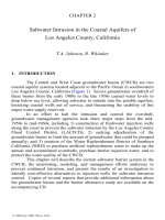
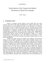
Figure 1: (a) Map of The Netherlands: position of the island of Texel and
ground surface of The Netherlands; (b) map of Texel: position of the four
polder areas and sand-dune area as well as phreatic water level in the top
aquifer at –0.75 m N.A.P. The polder area Eijerland was retrieved from the
tidal planes and created during the years 1835–1876. The two profiles refer
to Figures 8 and 9.
these water management problems and to gain a comprehensive, coherent
knowledge about the whole water system. In addition, technical measures
were suggested to control water management in the area. In this article, the
interest is only focused on a part of the study, viz. the density-driven
groundwater system under changing environmental conditions. The author of
this article constructed the density-driven groundwater system with the help
of Jeroen Tempelaars and Arco van Vugt.
First, the computer code, which is used to simulate variable density
flow in this groundwater system, is summarized. Second, the model of Texel

will be designed, based on subsoil parameters, model parameters, and
boundary conditions. The numerical results of the autonomous situation and
one scenario of sea level rise are discussed in the next section, and finally,
conclusions are drawn.
2. CHARACTERISTICS OF THE NUMERICAL MODEL
MOCDENS3D [Oude Essink, 1998] is used to simulate the transient
groundwater system as it occurs on the island of Texel. Originally, this code
was the three-dimensional computer code MOC3D [Konikow et al., 1996].
© 2004 by CRC Press LLC
Island of Texel, The Netherlands
79

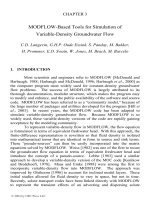
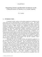
Figure 2: (a) A schematization of the hydrogeological situation at the island
of Texel, The Netherlands; (b) the simplified composition of the subsoil into
six main subsystems: one aquitard system and five aquifer systems (of which
the top three are intersected by aquitards).
2.1 Groundwater Flow Equation
The MODFLOW module solves the density-driven groundwater
flow equation [McDonald and Harbaugh, 1988; Harbaugh and McDonald,
1996]. It consists of the continuity equation combined with the equation of
motion. Under the given circumstances in the Dutch coastal aquifers, the
Oberbeck-Boussinesq approximation is valid as it is suggested that the
density variations (due to concentration changes) remain small to moderate
in comparison with the reference density
ρ
throughout the considered
hydrogeologic system:
yf
x
z

s
q
q
q
SW
xyz t
φ
∂
∂
∂
∂
++= +
∂∂∂ ∂

(1)
;
x
p
q
x
x
∂
∂
−=
µ
κ

;
y
p

q
y
y
∂
∂
−=
µ
κ

z
z
p
qg
z
κ
ρ
µ
∂

=− +

∂

(2)

where =
zyx
qqq ,, Darcian specific discharges in the principal directions
[
1

LT
−
]; S
s
= specific storage of the porous material [
1
L
−
]; W = source
function, which describes the mass flux of the fluid into (negative sign) or
© 2004 by CRC Press LLC
Coastal Aquifer Management
80
out of (positive sign) the system [
1
T
−
]; , ,
xyz
κ
κκ
=
principal intrinsic
permeabilities [
2
L ]; µ = dynamic viscosity of water [
11
M
LT
−

−
]; p = pressure
[
12
M
LT
−−
]; and g = gravitational acceleration [
2−
L
T
]. A so-called
freshwater head
f
φ
[L] is introduced to take into account differences in
density in the calculation of the head:
z
p
f
f
+=
g
ρ
φ
(3)
where
f
ρ

= the reference density [
3
M
L
−
], usually the density of fresh
groundwater at reference chloride concentration
0
C , and z is the elevation
head [
L].
Rewriting the Darcian specific discharge in terms of freshwater head
gives:
;
x
g
q
ffx
x
∂
∂
−=
φ
µ
ρ
κ

;
y
g

q
ffy
y
∂
∂
−=
φ
µ
ρ
κ









−
+
∂
∂
−=
f
fffz
z
z
g
q

ρ
ρρφ
µ
ρκ
(4)
In many cases small viscosity differences can be neglected if density
differences are considered in normal hydrogeologic systems [Verruijt, 1980;
Bear and Verruijt, 1987].
i
fi
k
g
=
µ
ρ
κ
(5)
;
f
xx
qk
x
φ
∂
=−
∂

;
f
yy

qk
y
φ
∂
=−
∂

f
f
zz
qk
z
φ
ρρ
ρ




∂
−
=− +
∂
(6)
The basic water balance used in MODFLOW is given below [McDonald and
Harbaugh, 1988]:
f
QS V
is
t

φ
∆
=
∆
∑
∆
(7)
where
Q
i

= total flow rate into the element (
31
LT
−
) and
∆
V = volume of the
element (
3
L ). The MODFLOW basic equation for density dependent
groundwater flow becomes as follows [Oude Essink, 1998, 2001]:
© 2004 by CRC Press LLC
Island of Texel, The Netherlands
81
1,,1 1 1,, 1 ,1,
,, ,, , ,
22 2
11 1
,, ,, , ,

22 2
11 1 ,,,,
,, ,, , ,
22 2
1,,1 1 1,,
,, ,,
22
(
)
tt tt tt
ijk i jk ij k
ijk i jk ij k
ijk i jk ij k
tt
ijk ijk
ijk i jk ij k
tt t
ijk i jk
ijk i jk
CV CC CR
CV CC CR
CV CC CR HCOF
CV CC
φφφ
φ
φφ
+∆ +∆ +∆
−− −
−− −
−− −

+∆
++ +
+∆ +
++
++
++
−++
++ +−
++
1,1, ,,
,,
2
ttt
ij k ijk
ij k
CR RHS
φ
∆+∆
+
+
+=

,, ,,
1
ijk ijk
HCOF P SC t
=
−∆
,, ,, ,, ,,
11,,1,,

,, ,,
22
1 1 ,, ,, 1
,, ,,
22
1
()2
()2
t
ijk ijk ijk ijk
ijk ijk
ijk ijk
ijk ijk
ijk ijk
RHS Q SC t
CV d d
CV d d
φ
−
−−
+
++
=− − ∆
−Ψ +
+Ψ +

,, ,,
1
ijk ijk
SC SS V=∆ (8)

,, 1 ,,
,, 1/2
,, ,, 1
,, 1/2
()2
()2
ijk ijk f
ijk
f
ijk ijk f
ijk
f
ρ
ρρ
ρ
ρ
ρρ
ρ
−
−
+
+

+−
Ψ=




+−

Ψ=



(9)
where
,, ,, ,,
,,
ijk ijk ijk
CV CC CR
=
the so-called MODFLOW hydraulic
conductance between elements in respectively vertical, column, and row
directions (
21
LT
−
) [McDonald and Harbaugh, 1988];
,, ,,
,
ijk ijk
PQ= factors
that account for the combined flow of all external sources and stresses into
an element (
21
LT
−
);
,,ijk
SS

=
specific storage of an element (
1
L
−
);
,,ijk
d =
thickness of the model layer k (L), and
,,ijk
Ψ
= buoyancy terms
(dimensionless). The two buoyancy terms
,,ijk
Ψ
are subtracted from the so-
called right head side term
,,ijk
R
HS to take into account variable density. See
Oude Essink [1998, 2001] for a detailed description of the adaptation of
MODFLOW to density differences.
2.2 The Advection-Dispersion Equation
The MOC module uses the method of characteristics to solve the
advection-dispersion equation, which simulates the solute transport
[Konikow and Bredehoeft, 1978; Konikow et al., 1996]. Advective transport
© 2004 by CRC Press LLC
Coastal Aquifer Management
82
of solutes is modeled by means of the method of particle tracking and

dispersive transport by means of the finite difference method:
()
()
'CCW
CC
R
DCV RC
dij i d
tx x x n
iji e
λ

−
∂∂ ∂ ∂

=−+−

∂∂ ∂ ∂



(10)
The used reference solute is chloride that is expected to be conservative.
MOCDENS3D takes into account hydrodynamic dispersion.
2.3 The Equation of State
A linear equation of state couples groundwater flow and solute
transport:
,, f C 0
[1 ( )]
ijk

CC
ρβ
ρ
=+ −
(11)
where
,,ijk
ρ
is the density of groundwater (
3
M
L
−
), C is the chloride
concentration (
3
M
L
−
), and
C
β
is the volumetric concentration expansion
gradient (
13
M
L
−
). During the numerical simulation, changes in solutes,
transported by advection, dispersion, and molecular diffusion, affect the

density and thus the groundwater flow. The groundwater flow equation is
recalculated regularly to account for changes in density.
2.4 Examples of Three-Dimensional Studies with MOCDENS3D
The computer code MOCDENS3D has recently also been used for
three other three-dimensional regional groundwater systems in The
Netherlands: (a) the northern part of the province of North-Holland: 65.0 km
by 51.25 km by 290 m with ~40,000 active elements [Oude Essink, 2001];
(b) the Wieringermeerpolder at the province of North-Holland: 23.2 km by
27.2 km by 385 m with ~312,000 active elements [Oude Essink, 2003; Water
board Uitwaterende Sluizen, 2001]; and (c) the water board of Rijnland in
the province of South-Holland: 52.25 km by 60.25 km by 190 m with
1,209,000 active elements [Oude Essink and Schaars, 2003; Water Board of
Rijnland, 2003].
3. MODEL DESIGN
3.1 Geometry, Model Grid, and Temporal Discretization
The following parameters are applied for the numerical
computations. The groundwater system consists of a three-dimensional grid
of 20.0 km by 29.0 km by 302 m depth. Each element is 250 m by 250 m
long. In vertical direction the thickness of the elements varies from 1.5 m at
© 2004 by CRC Press LLC
Island of Texel, The Netherlands
83
the top layer to 20 m over the deepest 10 layers (Figure 2b). The grid
contains 213,440 elements: n
x
= 80, n
y
= 116, n
z
= 23, where n

i
denotes the
number of elements in the i direction. Due to the rugged coastline of the
system and the irregular shape of the impervious hydrogeologic base, only
58.8% of the elements (125,554 out of 213,440) are considered as active
elements. Each active element contains eight particles to solve the advection
term of the solute transport equation. As such, some one million particles are
used initially. The flow timestep ∆t to recalculate the groundwater flow
equation equals 1 year. The convergence criterion for the groundwater flow
equation (freshwater head) is equal to 10
-5
m. The total simulation time is
500 years.
3.2 Subsoil Parameters
The groundwater system consists of permeable aquifers, intersected
by loamy aquitards and aquitards of clayey and peat composite (Figure 2b).
The system can be divided into six main subsystems. The top subsystem
(from 0 m to –22 m N.A.P.) and the second subsystem (from –22 m to –62 m
N.A.P.) have hydraulic conductivities k
x
of approximately 5 m/d and 30 m/d,
respectively. The third subsystem is an aquitard of 10 m thickness and has
hydraulic conductivities k
x
that varies from 0.01 to 1 m/d. The fourth
subsystem (from –72 m to –102 m N.A.P.) and fifth subsystem (from –102 m
to –202 m N.A.P.) have hydraulic conductivities k
x
of some 30 m/d and only
2 m/d, respectively. The lowest subsystem, number six, has a hydraulic

conductivity k
x
of approximately 10 m/d to 30 m/d. Note that the first,
second, and fourth subsystems are intersected by aquitards.
The following subsoil parameters are assumed: the anisotropy ratio
k
z
/k
x
equals 0.4 for all layers. The effective porosity n
e
is 0.35. The
longitudinal dispersivity
α
L
is set equal to 2 m, while the ratio of transversal
to longitudinal dispersivity is 0.1. For a conservative solute as chloride, the
molecular diffusion for porous media is taken equal to 10
-9
m
2
/s. Note that no
numerical “Peclet” problems occurred during the simulations [Oude Essink
and Boekelman, 1996]. On the applied time scale, the specific storativity S
s

(
1
L
−

) can be set to zero.
The bottom of the system as well as the vertical seaside borders is
considered to be no-flux boundaries. At the top of the system, the mean sea
level is –0.10 m N.A.P. and is constant in time in case of no sea level rise.
3



3
Note that in reality, the mean sea level in the eastern direction toward the Waddenzee is
probably somewhat higher over a few hundreds of meters. The reason is that at low tide, the
piezometric head in the phreatic aquifer of this tidal foreland outside the dike cannot follow
the relatively rapid tidal surface water fluctuations (Lebbe, pers. comm., 2000). It will be
retarded, which results in a higher low tide level of the sea, and thus in a higher mean sea
level.
© 2004 by CRC Press LLC
Coastal Aquifer Management
84
A number of low-lying areas are present in the system with a total area of
approximately 124 km
2
. The phreatic water level in the polder areas differs
significantly, varying from –2.05 m to +4.75 m N.A.P. at the hill De Hooge
Berg (Figure 1b), and is kept constant in time. Small fluctuations in the
phreatic water level are neglected. The constant natural groundwater
recharge equals 1 mm/d in the sand-dune area.
The volumetric concentration expansion gradient
C
β
is 1.34 ä 10

-6
l/mg Cl
-
. Saline groundwater in the lower layers does not exceed 18,000 mg
Cl
-
/l, as seawater that intruded the groundwater system has been mixed with
water from the river Rhine. The corresponding density of that saline
groundwater equals 1024.1 kg/m
3
.
3.3 Determination of the Initial Density Distribution
By 1990 AD, the hydrogeologic system contains saline, brackish as
well as fresh groundwater. On the average, the salinity increases with depth,
whereas freshwater lenses exist at the sand-dune areas at the western side of
the island, up to some –50 m N.A.P. A freshwater lens of some 50 m
thickness has evolved at the sandy hill De Hooge Berg.
Head as well as density differences affect groundwater flow in this
system. Density-driven groundwater flow simulated with a numerical model
is very sensitive to the accuracy of the initial density distribution. As such,
the initial chloride concentration, which is linearly related to the initial
density by Eq. (10), must be accurately inserted in each active element.
In this particular situation,
4
the present density distribution cannot be
deduced by simply simulating the saline groundwater system for many
hundreds of years with all actual load and concentration boundary
conditions, and waiting until the composition of solutes ceases to change.
The reason is that the present distribution of fresh, brackish, and saline
groundwater is still not in equilibrium. Several processes initiated in the past

can still be sensed and make the situation dynamic. For instance, during the
past centuries, the position of the island of Texel itself was not fixed
[Province of North-Holland, 2000]. It has slowly been moved, mainly from
the west to the east [Oost, 1995]. As a consequence, freshwater lenses in the
sand-dune areas could not follow the moving upper boundary conditions of
natural groundwater recharge. Moreover, other human activities such as
polders were created, some even from the 17
th
century on. Groundwater
extractions confirm the dynamic character of the island.
Therefore, from a practical point of view and based on the fact that
the system is still dynamic, chloride (and thus density) measurements at the


4
As a matter of fact, the same circumstances are present in most other coastal areas in The
Netherlands.
© 2004 by CRC Press LLC
Island of Texel, The Netherlands
85


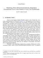
Figure 3: Calibration of the freshwater head: computed versus “measured”
freshwater heads.
year 1990 AD are chosen as the initial situation. Though this initial chloride
distribution in this Texel case is based on about 100 measurements of
chloride, errors can easily occur, mainly because of a lack of enough data.
Artificial inversions of fresh and saline groundwater can easily occur in the
numerical model, though they do not exist in reality. As a remedy, 10 years
are simulated under reference conditions (e.g., constant head at polders and

the sea), viz. from 1990 to 2000 AD. These years are necessary to smooth
out unwanted, unrealistic density dependent groundwater flow, which was
caused by the numerical discretization of the initial density distribution.
4. DISCUSSION
4.1 Calibration of the Model
Calibration of the numerical model was focused on the freshwater
heads in the hydrogeologic system, as well as on seepage and salt load values
that were measured at five pumping stations in the surface water system
[Province of North-Holland, 2000]. Freshwater head calibration was
executed by comparing 111 measured and simulated (freshwater) heads,

© 2004 by CRC Press LLC
Coastal Aquifer Management
86

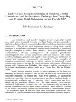
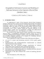
Figure 4: Chloride concentration in the top layer at
-0.75 m N.A.P. for the
years 2000 and 2200 AD. No sea level rise is simulated.
which were corrected for density differences. Figure 3 shows the head
calibration. The module PEST of PMWIN (version 5.0) was used to
minimize the difference between measured and simulated (freshwater) heads.
A sensitivity analysis has been executed on the following, in this system,
most important subsoil parameters: drainage resistance; streambed resistance
of the main water channels; vertical resistance of the Holocene aquitard in
the polder area; horizontal hydraulic conductivity of the phreatic aquifer in
the sand-dune area; and the vertical hydraulic conductivities of the aquitards
in aquifer systems two and three (see Figure 2b).
For all observation wells, the mean error was +0.07 m, the mean
absolute error 0.24 m, and the root mean square error 0.36 m. Systematic
errors were not assumed. Seasonal variations in natural recharge obstruct

easy calibration of the density dependent groundwater flow model with
seepage and salt load values.
Overall, more accurate model parameters, e.g., the increase of the
initial number of particles per element, a smaller timestep to recalculate the
velocity field, and a smaller convergence criterion for the groundwater flow
equation, did not significantly improve the numerical simulation of the
salinization process in the hydrogeologic system.
© 2004 by CRC Press LLC
Island of Texel, The Netherlands
87

Figure 5: Seepage through the top layer at
-0.75 m N.A.P. for the years 2000
and 2200 AD. Sea level rise is 0.75 meter per century.
4.2 Autonomous Saltwater Intrusion during the Period 2000–2200 AD
In the year 2000 AD, the chloride concentration is already high in
the four polder areas (Figure 4). At the hill De Hooge Berg, fresh
groundwater occurs up to some
-45 m M.S.L. Freshwater from the sand-
dunes flows toward the sea as well as toward the low-lying polder areas. In
these low-lying areas, seepage is quite high (up to some 2.1 mm/day at the
western side of the Prins Hendrik polder, see Figure 5a). In addition, the salt
load is high too, with values up to some 95,000 kg/ha/year in the same polder
area (Figure 6a).
The future autonomous salinization of the groundwater system of the
island of Texel is visualized in Figure 4. It shows the change in chloride
concentration in the top layer in the years 2000 AD and 2200 AD. The level
of sea is kept constant during these 200 years. The salinity in the top layer
increases, especially in the areas close to the coastline. The polders, which
were created at least 125 years ago, cause the salinity increase. The time lag

© 2004 by CRC Press LLC
Coastal Aquifer Management
88

Figure 6: Salt load (in kg/ha/year) in the top layer at
-0.75 m N.A.P. for the
years 2000 and 2200 AD. Sea level rise is 0.75 meter per century.
of the salinization process is considerable, at least many tens of years. The
animation of the concentration evolution is provided on the accompanying
CD.
4.3 Effect of Sea Level Rise on Saltwater Intrusion during the Next
500 Years
According to the Intergovernmental Panel of Climate Change
(IPCC) Second Assessment Report [Warrick et al., 1996], a sea level rise of
0.49 m is to be expected for the year 2100, with an uncertainty range from
0.20 to 0.86 m. This rate is 2 to 5 times the rate experienced over the last
century. One scenario of relative sea level variation is considered for the next
500 years: a relative sea level rise of 0.75 m per century. This figure includes
land subsidence caused by groundwater recovery, the compaction and
shrinkage of clay, and especially the oxidation of peat.

© 2004 by CRC Press LLC
Island of Texel, The Netherlands
89

Figure 7: Chloride concentration in the top layer at
-0.75 m N.A.P. for the
years 2200 and 2500 AD. Sea level rise is 0.75 m per century.
Figure 7 shows the change in chloride concentration in the top layer

at
-0.75 m N.A.P. for the sea level rise scenario at two moments in time: 200
years (2200 AD) and 500 years (2500 AD) after 2000 AD. During the next
centuries, the salinity in the groundwater system will increase very seriously
when the sea level rises by 0.75 m/c.
The same process can obviously be detected in a cross-section; see
Figure 8 (west-east direction) and Figure 9 (north-south direction). The exact
positions of the profiles in these figures are given in Figure 1b. The effect of
a sea level rise relative to no sea level rise on the chloride concentration in
the top layer can be deduced by comparing Figures 4b and 7a: the salinity
increases more rapidly in the low-lying polder areas. The freshwater lenses at
the sand-dune area as well as at the hill De Hooge Berg remain, though these
lenses become less deep.
Seepage in the polders (Figure 5) as well as the salt load (Figure 6) at
-0.75 m N.A.P. increase as a function of time. Two processes cause the
increase of salt load: the increase of seepage as well as the increase in
salinity of the top hydrogeologic system. The polder areas attract seawater,
with a high content of chloride, as the phreatic water level in these areas is
low relative to the level of the sea.
© 2004 by CRC Press LLC
Coastal Aquifer Management
90

Figure 8: Chloride concentration in a cross-section in western-eastern
direction (row 76) for the years 2000, 2200, and 2500 AD, over the hill De
Hooge Berg. Only the top system up to
-102 m N.A.P. is shown. The
relative sea level rise is 0.75 m per century. The arrows correspond with the
displacement of groundwater during a time step of 20 years.
In Figure 10, the seepage in the four different polder areas is given

as a function of time. As can be seen, seepage quantities increase, which will
probably have its effect on the capacity of the pumping stations in the polder
areas. Their capacity should be increased because, e.g., in 200 years, the
seepage quantity is about doubled in all four areas.
The salt load as a function of time demonstrates that the effect of sea
level rise is substantial in all four low-lying polder areas of the island of
Texel (Figure 11). The increase in salt load will be enormous due to the sea
level rise of 0.75 m per century. This will definitely affect environmental
aspects. A doubling of the salt load is probably already reached within (only)
one century in the polder areas Eijerland and Dijksmanhuizen.


© 2004 by CRC Press LLC
Island of Texel, The Netherlands
91

Figure 9: Chloride concentration in a cross-section in northern-southern
direction (column 45) for the years 2000, 2200, and 2500 AD. Only the top
system up to
-102 m N.A.P. is shown. The relative sea level rise is 0.75 m
per century. The arrows correspond with the displacement of groundwater
during a time step of 20 years.
5. CONCLUSIONS
The “Great Geohydrological Research Texel” was initiated to
investigate the effect of environmental and anthropogenic stresses on the
groundwater system at the island of Texel. Differences in present water level
between the sea and low-lying polders of the island of Texel suggest a large
inflow of seawater toward the land. A numerical model was constructed to
quantify this phenomenon and to assess the effect of future physical stresses
such as sea level rise and land subsidence on the groundwater system. The

computer code MOCDENS3D was used to simulate density dependent
groundwater flow at the island of Texel in three dimensions with a surface of
130 km
2
by 300 m thickness. The reliability of the numerical model highly
depends on the quality of especially the initial density distribution.
Numerical computations show that saltwater intrusion is severe because the

© 2004 by CRC Press LLC
Coastal Aquifer Management
92

Figure 10: Seepage (in m3/day) through the top layer at
-0.75 m N.A.P. of
the four polder areas as a function of 500 years.

Figure 11: Salt load (in ton Cl
-
/year) through the top layer at -0.75 m N.A.P.
of the four polder areas as a function of 500 years.


© 2004 by CRC Press LLC
Island of Texel, The Netherlands
93
polder areas with low phreatic water levels are situated very close to the sea.
When the sea level rises relatively 0.75 m per century, the increase in salinity
is enormous. A doubling of the present seepage quantities can be established
within two centuries in all four polder areas. Moreover, the salt load will
probably be doubled in two polder areas within only one century. This will

definitely affect environmental, as well socio-economic aspects of the island
of Texel.
Acknowledgments
The author wishes to thank Jeroen Tempelaars and Arco van Vugt of
the consulting engineering company Witteveen & Bos, The Netherlands, for
the preparation of the input files (especially subsoil parameters) for the
numerical model, as well as executing the sensitivity analysis of subsoil
parameters.
REFERENCES
Bear, J. and Verruijt, A., Modeling Groundwater Flow and Pollution, D.
Reidel Publishing Company, Dordrecht, The Netherlands, 414 p.,
1987.
Harbaugh, A.W. and McDonald, M.G., User's documentation for the
U.S.G.S. modular finite-difference ground-water flow model,
U.S.G.S. Open-File Report 96-485, 56 p., 1996.
Water board Uitwaterende Sluizen, “Geohydrological Research
Wieringerrandmeer”, by the consulting engineering company
Grontmij Noord-Holland, on behalf of the Water board Uitwaterende
Sluizen by order of the steering committee “Water Bindt”, 48 p.,
2001.
Konikow, L.F. and Bredehoeft, J.D., Computer model of two-dimensional
solute transport and dispersion in ground water; U.S.G.S. Tech. of
Water-Resources Investigations, Book 7, Chapter C2, 90 p., 1978.
Konikow, L.F., Goode, D.J., and Hornberger, G.Z., A three-dimensional
method-of-characteristics solute-transport model (MOC3D);
U.S.G.S. Water-Resources Investigations Report 96-4267, 87 p.,
1996.
McDonald, M.G. and Harbaugh, A.W., A modular three-dimensional finite-
difference ground-water flow model; U.S.G.S. Techniques of Water-
Resources Investigations, Book 6, Chapter A1, 586 p., 1988.

Oost, A.P., “Dynamics and sedimentary development of the Dutch Wadden
Sea with emphasis on the Frisian Inlet”, Ph.D. dissertation, Utrecht
University, 445 p., 1995.
© 2004 by CRC Press LLC
Coastal Aquifer Management
94
Oude Essink, G.H.P., “MOC3D adapted to simulate 3D density-dependent
groundwater flow,” In: Proc. MODFLOW'98 Conf., Golden, CO,
291–303, 1998.
Oude Essink, G.H.P., “Density dependent groundwater flow at the island of
Texel, The Netherlands” In: Proc. 16th Salt Water Intrusion
Meeting, Miedzyzdroje-Wolin Island, Poland, June 2000, 47–54,
2001.
Oude Essink, G.H.P., “Salt Water Intrusion in a Three-dimensional
Groundwater System in The Netherlands: a Numerical Study,”
Transport in Porous Media,
43 (1), 137–158, 2001.
Oude Essink, G.H.P., “Salinization of the Wieringermeerpolder, The
Netherlands” In: Proc. 17th Salt Water Intrusion Meeting, Delft, The
Netherlands, 399–411, 2003.
Oude Essink, G.H.P. and Schaars, F., “Impact of climate change on the
groundwater system of the water board of Rijnland, The
Netherlands” In: Proc. 17th Salt Water Intrusion Meeting, Delft, The
Netherlands, 379–392, 2003.
Oude Essink, G.H.P. and Boekelman, R.H., “Problems with large-scale
modeling of salt water intrusion in 3D,” In: Proc. 14th Salt Water
Intrusion Meeting, Malmö, Sweden, June 1996, 16–31, 1996.
Province of North-Holland, “Great Geohydrological Research Texel”, by the
consulting engineering company Witteveen & Bos, on behalf of the
Province of North-Holland, the Water board Hollands Kroon, the

city Texel and the Water board Uitwaterende Sluizen, 73 p., 2000.
Verruijt, A., “The rotation of a vertical interface in a porous medium,” Water
Resour. Res.,
16 (1), 239–240, 1980.
Warrick, R.A., Oerlemans, J., Woodworth, P., Meier, M.F., and Le Provost,
C., “Changes in sea level,” In: Climate Change 1995: The Science of
Climate, eds. J.T. Houghton, L.G. Meira Filho, and B.A. Callander,
Contribution of Working Group I to the Second Assessment Report
of the Intergovernmental Panel of Climate Change, 359–405,
Cambridge Univ. Press, Cambridge, 1996.
Water Board of Rijnland, “The salt of the earth”, by KIWA research and
consultancy, on behalf of the Water Board of Rijnland, 2003.
© 2004 by CRC Press LLC