COASTAL AQUIFER MANAGEMENT: monitoring, modeling, and case studies - Chapter 11 potx

CHAPTER 11
Pumping Optimization in Saltwater-Intruded Aquifers
A.H D. Cheng, M.K. Benhachmi, D. Halhal, D. Ouazar, A. Naji,
K. EL Harrouni
1. INTRODUCTION
Coastal aquifers serve as major sources for freshwater supply in
many countries around the world, especially in arid and semiarid zones.
Many coastal areas are heavily urbanized, a fact that makes the need for
freshwater even more acute [Bear and Cheng, 1999]. Inappropriate
management of coastal aquifers may lead to the intrusion of saltwater into
freshwater wells, destroying them as sources of freshwater supply. One of
the goals of coastal aquifer management is to maximize freshwater extraction
without causing the invasion of saltwater into the wells.
A number of management questions can be asked in such
considerations. For existing wells, how should the pumping rate be
apportioned and regulated so
as to achieve the maximum total extraction?
For new wells, where should they be located and how much can they pump?
How can recharge wells and canals be used to protect pumping wells, and
where should they be placed? If recycled water is used in the injection, how
can we maximize the recovery percentage? These and other questions may
be answered using the mathematical tool of optimization.
Efforts to improve the management of groundwater systems by
computer simulation and optimization techniques began in the early 1970s
[Young and Bredehoe, 1972; Aguado and Remson, 1974]. Since that time, a
large number of groundwater management models have been successfully
applied; see for example Gorelick [1983], Willis and Yeh [1987], and many
other papers published in the Journal of Water Resources Planning and
Management, ASCE, and the Water Resources Research. Applications of
these models to aquifer situations with the explicit threat of saltwater

intrusion in mind, however, are relatively few [Cumming, 1971; Cummings
and McFarland, 1974; Shamir et al., 1984; Willis and Finney, 1988; Finney
et al., 1992; Hallaji and Yazicigil, 1996; Emch and Yeh, 1998; Nishikawa,
© 2004 by CRC Press LLC
Coastal Aquifer Management
234
1998; Das and Datta, 1999a, 1999b; Cheng et al., 2000]. In terms of
management objectives, some of these studies have addressed relatively
complex settings such as mixed use of surface and subsurface water in terms
of quantity and quality, water conveyance, distribution network, construction
and utility costs, etc. However, saltwater intrusion into wells has been dealt
with in simpler and indirect approaches, for example, by constraining
drawdown or water quality at a number of control points, or by minimizing
the overall intruded saltwater volume in the entire aquifer. The explicit
modeling of saltwater encroachment into individual wells resulting in the
removal of invaded wells from service is found only in Cheng et al. [2000].
This chapter reviews some of the earlier considerations of pumping
optimization in saltwater-intruded aquifers under deterministic conditions,
and furthermore, introduces the uncertainty factor into the management
problem. The resultant methodology is applied to the case study of the City
of Miami Beach in the northeast Spain.
2. DETERMINISTIC SIMULATION MODEL
The first step of modeling is to have a physical/mathematical model.
Depending on the available data input from the field problem and the
desirable outcome of the simulation, models of different levels of
complexity, ranging from the sharp-interface model to the density-dependent
miscible transport model, can be used [Bear, 1999]. For the method of
solution, it can range from simple analytical solutions [Cheng and Ouazar,
1999] to the various finite-element- and finite-difference-based numerical
solutions [Sorek and Pinder, 1999]. In principle, any of the above models and

methods can be used; in reality, however, the selection of the model is
dependent on the tolerable computer CPU time, as both the optimization and
the stochastic modeling can be computational time consuming.
In our case, the Genetic Algorithm (GA) has been chosen as the
optimization tool. Due to the large number of individual simulations needed
in the GA, the simulation model needs to be highly efficient in order to stay
within a reasonable amount of computation time. For this reason, the sharp
interface analytical solution is chosen, which is briefly described in the
following.
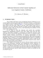
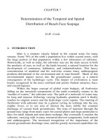
Figures 1(a) and (b) respectively give the definition sketch of a
confined and an unconfined aquifer. The aquifers are with homogeneous
hydraulic conductivity K and constant thickness B in the confined aquifer
case. Distinction has been made between two zones—a freshwater only zone
(zone 1), and a freshwater–saltwater coexisting zone (zone 2). Following the

© 2004 by CRC Press LLC
Pumping Optimization in Saltwater-Intruded Aquifers
235

Figure 1: Definition sketch of saltwater intrusion in (a) a confined aquifer,
and (b) an unconfined aquifer.
work of Strack [1976], the Dupuit-Forchheimer hydraulic assumption is used
to vertically integrate the flow equation, reducing the solution geometry from
three-dimensional to two-dimensional (horizontal x-y plane). Steady state is
assumed. The Ghyben-Herzberg assumption of stagnant saltwater is utilized
to find the saltwater–freshwater interface. With the above common
assumptions of groundwater flow, the governing equation for the system is
the Laplace equation:

2

0
φ
∇
= (1)
where
2
∇ is the Laplacian operator in two-spatial dimensions (x and y), and
the potential
φ
is defined differently in the two zones
© 2004 by CRC Press LLC
Coastal Aquifer Management
236
y
saltwater
invaded
zone
freshwater
zone
pumping well
inactive well
toe
(x y )
ii
,
Q
i
q
coastline
sea

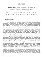
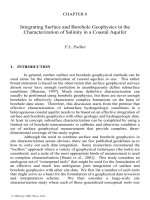
Figure 2: Pumping wells in a coastal aquifer.

2
2
1
[ ( 1) ] for zone 1
2( 1)
1
[(1) ]for zone 2
2( 1)
ff
f
Bh h s B sd
s
hsBsd
s
φ
φ
== +−−
−
=+−−
−
(2)
for confined aquifer; and

22
2
1

[ ] for zone 1
2
( ) for zone 2
2( 1)
f
f
hsd
s
hd
s
φ
φ
=−
=−
−
(3)
for unconfined aquifer. We also define

s
s
f
ρ
ρ
=
(4)
as the saltwater and freshwater density ratio, and other definitions are found
in Figure 1.
In our problem, we consider a semi-infinite coastal plain bounded by
a straight coastline aligned with the y-axis (Figure 2). Multiple pumping
x

x
w
Qq
toe
coastline
wellx
xw
Qq
toe
coastline
well
x
x
w
Qq
toe
coastline
wellx
xw
Qq
toe
coastline
wellx
xw
Qq
toe
coastline
wellx
xw
Qq

toe
coastline
wellx
xw
Qq
toe
coastline
wellx
xw
Qq
toe
coastline
well
© 2004 by CRC Press LLC
Pumping Optimization in Saltwater-Intruded Aquifers
237
wells are located in the aquifer with coordinates (, )
ii
x
y and discharge
i
Q .
There is a uniform freshwater outflow rate
q. The aquifer can be confined or
unconfined. Solution of the potential
φ
for this problem can be found by the
method of images and has been given by Strack [1976] (see also Cheng and
Ouazar, 1999):

22
22
1
()( )
ln
4
()( )
n
iii
i
ii
Qxxyy
q
x
KK
xx yy
φ
π
=


−+−
=+


++−


∑
(5)

With the above solution, the toe location of saltwater wedge
toe
x
is found
where the potential takes the value
toe
φ
,

22
22
1
()()
ln
4
()()
toe
n
toe toe
iii
toe
i
ii
Qxxyy
q
x
KK
xx yy
φ
π

=


−+−
=+


++−


∑
(6)
where

2
1
for confined aquifer
2
toe
s
B
φ
−
=

2
(1)
for unconfined aquifer
2
toe

ss
d
φ
−
= (7)
Since
toe
φ
is some known number evaluated from Eq. (7), Eq. (6) can be
solved for
toe
x
for each given y value using a root finding technique.
3. OPTIMIZATION UNDER DETERMINISTIC CONDITIONS
The management objective of the coastal pumping operation is to
maximize the economic benefit from the pumped water less the utility cost
for lifting the water. For simplicity, we assume that the value of water and
the utility cost are both linear functions of discharge
i
Q . The objective is to
maximize the benefit function Z with respect to the design variables
i
Q
[Haimes, 1977]:

()
i
Q
1
max Z

n
ip Pi i
i
QB C L h
=


=−−


∑
(8)
In the above
p
B
is the economic benefit per unit discharge,
p
C is the cost
per unit discharge per unit lift height,
i
L is the ground elevation at well i,
and
i
h is the water level in well i. It should be remarked that although a
relative simple model is used for the right-hand side of Eq. (8), it can be
© 2004 by CRC Press LLC
Coastal Aquifer Management
238
generalized to a realistic microeconomic model involving supply and
demand without complicating the solution process.

The pumping operation is subject to some constraints. First, the
discharge of each well must stay within the certain limits set by the operation
conditions such as the minimum feasible pumping rate, maximum capacity
of the pump, restriction on well drawdown, etc. This can be written as

min max
or 0; for 1, ,
iii i
QQQ Q i n≤≤ = =… (9)
We note that the second condition in the above allows the well to be shut
down. Second, it is required that saltwater wedge does not invade the
pumping wells
at ; for all active wells
toe
ii i
xx yy<= (10)
where
toe
i
x
stands for the toe location in front of well i.
Since genetic algorithm can only work with unconstrained problems,
it is necessary to convert the constrained problem described by Eqs. (8)-(9)
to an unconstrained one. This is accomplished by the adding penalty to the
objective function for any violation that takes place:

()
2
1
max Z 1

i
toe
n
i
ip Pi i ii
Q
i
i
x
QB C L h rN
x
=


=−−−−



∑
(11)
where
i
r are penalty factors, which are empirically selected, and 1
i
N = for
toe
ii
x
x≥ and 0
i

N = for
toe
ii
x
x
<
. We notice that the constraint Eq. (9) is not
included in Eq. (11) because it is automatically satisfied by setting the
population space in genetic algorithm.
4. GENETIC ALGORITHM
Conventional optimization techniques, such as the linear and
nonlinear programming, and gradient-based search techniques are not
suitable for finding global optimum in space that is discontinuous and
contains a large number of local optima, which are the prevalent conditions
for the optimization problem defined above. To overcome these difficulties,
a genetic algorithm (GA) has been introduced and successfully applied
[Cheng et al., 2000]. GA is a probabilistic search based optimization
technique that imitates the biological process of evolution [Holland, 1975].
Its application to groundwater problems started in the mid-1990s [McKinney
and Lin, 1994; Ritzel et al., 1994; Rogers and Fowla, 1994; Cienlawski et
al., 1995], and since that time it has found many applications. (See Ouazar
and Cheng [1999] for a review.)
© 2004 by CRC Press LLC
Pumping Optimization in Saltwater-Intruded Aquifers
239
A brief illustration of the GA solution procedure applied to the
current problem is given below. Given the solution space of
i
Q defined by
Eq. (9), we discretize it in order to reduce the number of trial solutions from

infinite to a finite set. As an example, if each discharge is constrained
between 100 500
i
Q≤≤ m³/day, and the desirable accuracy of the solution is
5 m³/day (which is a rather crude resolution), then for each
i
Q there exist 82
possible discrete values (including the zero pumping rate). If there are 10
wells in the field, then the total number of possible combinations of pumping
rate is
10 19
82 1.4 10=× . One of the combinations is the optimal pumping
solution we look for. This search space is so huge that if we spend 1 sec of
CPU time to conduct a single simulation to check its benefit, it will take
11
410× years to complete the work. The search space of a typical field
problem in fact is greater than the above. Hence we must follow some
intelligent rules in the search; this is where the GA comes in.
GA seeks to represent the search space by binary strings. In the
above example, it is sufficient to represent all possible combinations of
pumping rate by a 64-bit binary string (
64 19
21.810=× ). To seed an initial
population, a random number generator is used to flip the bits between 0 and
1 to create individuals in the form of 01101…10111 (64 digits long), each
one corresponding to a distinct set of pumping rates. Typically a relatively
small number of individuals, say 10 to 20, are created to fill a generation.
Individuals are then tested for their fitness to survive by running the
deterministic simulation as described above. The fitness is determined by the
objective function given as the right-hand side of Eq. (11).

Once the fitness is determined for each individual in the generation,
certain evolutional-based probabilistic rules are applied to breed better
offspring. For example, in a simple genetic algorithm (SGA), three rules,
selection, crossover, and mutation, are used [Michalewicz, 1992]. First, the
selection process decides whether an individual will survive by “throwing a
dice” using a probability proportional to the individual’s fitness value.
Second, the GA disturbs the resulting population by performing crossover
with a probability of
c
p
. In this operation, each binary string (individual) is
considered as a chromosome. Segments of chromosome between individuals
can be exchanged according to the predetermined probability. Third, to
create diversity of the solution, GA further perturbs the population by
performing mutation with a probability of
m
p
. In this operation, each bit of
the chromosome is subjected to a small probability of mutation by allowing
it to be flipped from 1 to 0 or the other way around. After these steps, a new
generation is formed and the evolution continues. The process is terminated

© 2004 by CRC Press LLC
Coastal Aquifer Management
240
1
2
3
4
5

6
7
89
10
11
12
13
14
15
0
1000
2000
3000
4000
-3000
-2500
-2000
-1500
-1000
-500
0
500
1000
1500
2000
2500
y (m)
Coastline
x (m)
pumping well

toe
Inactive well

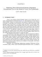
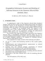
Figure 3: Pumping wells in a coast and saltwater intrusion front.
by a number of criteria, such as no improvement observed in an number of
generations, or reaching a pre-determined maximum number of generation.
The reader can consult the above-cited references for more detail.
5. EXAMPLE OF DETERMINISTIC OPTIMIZATION
This test case was examined in Cheng et al. [2000]. Assume an
unconfined aquifer with K = 40 m/day, q = 40 m²/day, d = 15 m,
s
ρ
= 1.025
g/cm³, and
f
ρ
= 1 g/cm³. Figure 3 gives an aerial view of the coast and the
locations of 15 pumping wells. The well coordinates are shown in columns
(2) and (3) of Table 1. Each well is bounded by a maximum and a minimum
well discharge, as indicated in columns (4) and (5). In this optimization
problem, only the benefit from the pumped volume is considered, and the
utility cost is neglected. The objective function (11) is modified to

2
1
max Z 1
i
toe
n
i

iii
Q
i
i
x
QrN
x
=

=− −


∑
(12)
© 2004 by CRC Press LLC
Pumping Optimization in Saltwater-Intruded Aquifers
241
(1) (2) (3) (4) (5) (6) (7)
Well
i
x

i
y
max
i
Q
min
i
Q

i
Q
toe
i
x

Id (m) (m) (m
3
/day) (m
3
/day) (m
3
/day) (m)
1 1000 2500 600 150 201 836
2 1700 1100 1300 150 351 1117
3 1500 850 1100 150 0 1257
4 1200 400 800 150 0 1372
5 1700 200 1300 150 150 1514
6 1800 -300 1400 150 0 1344
7 3500 -500 1500 150 1497 1323
8 1600 -800 1200 150 0 1311
9 1600 -1200 1200 150 0 1315
10 1500 -1600 1100 150 0 1332
11 2000 -2000 1500 150 155 1319
12 1000 -2200 600 150 0 1287
13 1600 -2500 1200 150 0 1241
14 3600 -2800 1500 150 1387 1251
15 1400 -3000 1000 150 150 1213
Total 3891
Table 1: Optimal pumping well solution.

The GA described earlier is used for optimization. In the first attempt, the
optimization was conducted by assuming all 15 wells are in operation. The
search space for each well is defined between
min
i
Q and
max
i
Q with increment
size of roughly 1 m³/day and also the zero discharge. If a well is invaded, a
penalty is imposed with an empirical penalty factor
i
r to discourage such
events. If the well is shut down, 0Q
=
, the program detects it and no penalty
is applied for invasion. This allows the inactive wells to be intruded in order
to increase pumping.
After three runs of GA with different seeding of initial population,
the best solution gives the total discharge of 3,610 m³/day. The optimal
solution shows that eight wells are in operation and seven are shut down. The
fact that so many wells are shut down is not surprising, as an estimate based
on a simple analytical solution [Cheng et al., 2000] shows that the well field
is too crowded and some wells can be taken out of action.
The program was run on a Pentium 450MHz microcomputer. It was
terminated when the maximum number of generations was reached, for about
6 hours of CPU time. Since an near optimal solution may not have been
reached, a second search is conducted using a refined strategy. In the second
search, only cases with any combinations of seven, eight, and nine wells in
© 2004 by CRC Press LLC

Coastal Aquifer Management
242
operation are admitted into the search space. Wells not selected do not exist
and can be invaded. This strategy much reduces the size of the search space
and better solution is obtained. The best solution is a seven-well case as
shown in column (6) of Table 1. The toe location in front of the wells is
shown in column (7). The total pumping rate is 3,891 m³/day. The saltwater
intrusion front is graphically demonstrated in Figure 3, with the well
locations marked. We notice that two of the inactive wells, 4 and 12, are
intruded by saltwater.
6. STOCHASTIC SIMULATION MODEL
The solution presented above assumes deterministic conditions, i.e.,
all aquifer data are known with certainty. This is not true in reality as
hydrogeological surveys are expensive and time consuming to conduct;
hence hydrogeological data are rare. The optimization model needs to take
this reality into consideration.
The first step of conducting a stochastic optimization is to have a
stochastic simulation model. This can be accomplished by applying the
second order uncertainty analysis of Cheng and Ouazar [1995] to the
deterministic model given as Eq. (6). Based on the approximation of Taylor
series, the statistical moments of toe location can be related to the moments
of uncertain parameters as [Naji et al., 1998]

()
22
22
22
1
,
2

toe toe
toe toe
qK
xx
xxqK
qK
σ
σ


∂∂
=+ +


∂∂


(13)

22
222
toe toe
x
qK
xx
qK
σ
σσ
 
∂∂

=+
 
∂∂
 
(14)
where
toe
x
, q , and K are respectively the mean toe location, the mean
freshwater outflow rate, and the mean hydraulic conductivity;
2
x
σ
,
2
q
σ
, and
2
K
σ
are respectively the variance of toe location, freshwater outflow rate, and
hydraulic conductivity; and
(
)
,
toe
x
qK is the toe location evaluated using the
mean parameter values. In the above, we have neglected the covariance

qK
σ

by assuming that it is small. The above equations state that in order to obtain
the mean toe location and its standard deviation, we first need to calculate
the toe location using the mean parameter values, i.e.,
(
)
,
toe
x
qK . This is
obtained from the deterministic solution by solving Eq. (6) using the given
q and K values. Next, we need to find the partial derivatives of toe location
© 2004 by CRC Press LLC
Pumping Optimization in Saltwater-Intruded Aquifers
243
with respect to q and K. This is found by perturbing the q and K values by
small amounts in Eq. (6). In other words, Eq. (6) is solved for the toe
location using values of
qq
±
∆ and KK
±
∆ and the difference in
toe
x
is
found. Utilizing finite difference approximation, the partial derivative
/

toe
x
q∂∂,
22
/
toe
x
q∂∂, etc., can be approximated. Given the variances of
aquifer data,
2
q
σ
and
2
K
σ
, we can then assemble the mean toe location and its
standard deviation from Eqs. (13) and (14). More detail of the above
procedure can be found in Cheng and Ouazar [1995], and Naji et al. [1998,
1999].
7. CHANCE CONSTRAINED OPTIMIZATION
The optimization problem described in Sections 2 through 5 is based
on deterministic conditions. In the event of input data uncertainty, a
stochastic optimization is necessary. The chance-constrained programming
[Charnes and Cooper, 1959; 1963] is used for this purpose. This optimization
model allows us to use stochastic parameters as input data and produces an
output prediction based on desirable reliability level.
Charnes and Cooper [1959, 1963] studied chance constrained
programming by transforming a stochastic optimization problem into a
deterministic equivalent. The chance-constrained programming can

incorporate reliability measures imposed on the decision variables. This
methodology has been applied to solve a number of groundwater
management problems. Tung [1986] developed a chance-constrained model
that takes into account the random nature of transmissivity and storage
coefficient. Wagner and Gorelick [1987] presented a modified form of the
chance constrained programming to determine a pumping strategy for
controlling groundwater quality. Hantush and Marino [1989] presented a
chance-constrained model for stream-aquifer interaction. Morgan et al.
[1993] developed a mixed-integer chance-constrained programming and
demonstrated its applicability to groundwater remediation problems. Chance-
constrained groundwater management models have also been applied to
design groundwater hydraulics [Tiedman and Gorelick, 1993] and quality
management strategies [Gailey and Gorelick, 1993]. Chan [1994] developed
a partial infeasibility method for aquifer management. Datta and Dhiman
[1996] utilized a chance-constrained model for designing a groundwater
quality monitoring network. Wagner [1999] employed the chance-
constrained model for identifying the least cost pumping strategy for
remediating groundwater contamination. Sawyer and Lin [1998] considered
the combination of uncertainty in the cost coefficients and constraints of the
groundwater management model.
© 2004 by CRC Press LLC
Coastal Aquifer Management
244
For the present problem we assume that the freshwater outflow rate q
and the hydraulic conductivity K are random variables, causing the toe
location in front of each well
toe
i
x
to be uncertain. The constraint given by

Eq. (10) needs to be modified to a probabilistic one:

(
)
Prob ; for all active wells
toe
ii
xxR<≥ (15)
where R is the desirable reliability level of prediction set by the water
manager. The chance constraint converts the above probabilistic constraint
into a deterministic one:

1
( ) ; for all active wells
toe
i
toe
ii
x
xFR x
σ
−
+< (16)
where
toe
i
x
is the expectation and
toe
i

x
σ
is the standard deviation of the toe
location
toe
i
x
, and
1
()
F
R
−
is the value of the standard normal cumulative
probability distribution corresponding to the reliability level R. The chance-
constrained optimization problem is then defined by the objective function
Eq. (8), which is subject to the constraints Eqs. (9) and (16).
In order to apply GA for the solution of the optimization problem,
we need to convert the constrained problem to an unconstrained one. Similar
to the deterministic problem, this is accomplished by imposing penalty for
the violation of the chance constraint Eq. (16):

()
2
1
1
()
max Z 1
toe
i

i
toe
n
i
x
ip Pi i ii
Q
i
i
xFR
QB C L h rN
x
σ
−
=

+


=−−− −



∑
(17)
which can be compared to its deterministic counterpart Eq. (11). The GA
methodology as described in Section 4 is then applied for its solution.
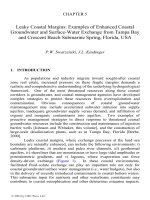
8. CASE STUDY—MIAMI BEACH, SPAIN
The above-proposed optimization model has been tested and applied
to a few hypothetical as well as real cases [Benhachmi et al., 2003a, b]. Here,

we report the case study of the city of Miami Beach in northeast Spain.
A large fraction of the total population of Spain (about 80% of its 6
million inhabitants) lives along the Catalonia coast [Bayó et al., 1992]. This
concentration of population creates large freshwater demands for domestic
consumption, in addition to the agricultural, industrial, and tourism needs.
Aquifers along the coast have been subjected to intensive exploitation;

© 2004 by CRC Press LLC
Pumping Optimization in Saltwater-Intruded Aquifers
245

Figure 4: Location of Miami Beach, Spain.
consequently, excessive salinity in well water is a common occurrence [Bayó
et al., 1992; Himmi, 2000]. In many situations, there is a poor understanding
of aquifer response, detailed studies are lacking, and the monitoring of
seawater intrusion is insufficient. In spite of the strict regulations introduced
in the Water Act of Spain, control of abstractions is scarce. In the coastal
area of Tarragona, north to Ebre, saltwater intrusion is caused by the
concentrated abstraction near the coast, which has contaminated many wells
and forced the freshwater importation of up to 4 m³/s from the Ebre river by
means of an 80 km canal and pipeline.
The current situation is in part a result of inadequate water resources
planning and management. The unfortunate consequence of management
failure is that there generally exists distrust in the public in the feasibility of
using coastal groundwater resources to meet water demands, and solutions
that need large amounts of investment are rejected. However, it is believed
that with adequate management and enforcement, some of the current
problems can be alleviated.
In the present work, we shall apply the previously described
stochastic optimization approach to the management of the Miami

© 2004 by CRC Press LLC
Coastal Aquifer Management
246

Figure 5: City of Miami Beach, Spain, and pumping well locations.
unconfined aquifer located near Tarragona, Spain (Figure 4). For many
years, the aquifer has been one of the most important water-supply sources
for the city of Miami Beach for domestic purposes. The study area is located
southwest of the city of Tarragona and encompasses about 17 km². Lithology
of Miami aquifer consists of unconsolidated sediments of Quaternary

© 2004 by CRC Press LLC
Pumping Optimization in Saltwater-Intruded Aquifers
247
(1)
No.
(2)
Well Id
(3)
x
w

(m)
(4)
y
w

(m)
(5)

Q
max
(m
3
/day)
(6)
Q
min
(m
3
/day)

(7)
L
i

(m)

1 Bonmont P4 3877 4362 1200 120 80
2 Bonmont P2 3826 3748 1200 120 113
3 Bonmont P5 3655 3390 1200 120 111
4 Urb. Casalot P4 3625 2648 1200 120 89
5 Bonmont P3 3507 3686 1200 120 81
6 Bonmont P1 3469 3900 1200 120 78
7 Bonmont P6 3285 4148 1200 120 66
8 S. Exterior 3161 4715 1200 120 67
9 Urb. Casalot P3 3133 2593 1200 120 85
10 Tapies 3 2808 961 1200 120 91
11 Urb. Casalot P2 2744 2705 1200 120 70
12 Tapies 2 2647 759 1200 120 89

13 Iglesias 2047 2496 1200 120 65
14 Zefil 1 1322 2922 1200 120 25
15 Ayu. De Miami 1246 2541 1200 120 30
16 Zefil 2 1077 2769 1200 120 22
17 Guardia Civil 906 2761 1200 120 19
18 Urb. Las Mimosas 873 4202 1200 120 20
19 La Florida 704 763 1200 120 34
20 Pozo de Sra. Mercedes 431 677 1200 120 20
21 C. Terme 358 672 1200 120 15
22 C. Miramar 304 4564 1200 120 12
23 Pino Alto 3 244 399 1200 120 13
24 Urb. Euromar 206 315 1200 120 14
25 Rio Llastres 179 101 1200 120 12
Table 2: Pumping well locations and discharge limits for the Miami Beach
aquifer.
age, corresponding to coastal piedmonts and alluvial fans, and is generally
unconfined and single-layered. The sediment consists of clay and gravel, and
overlies a blue clay of Pliocene age, which constitutes the effective lower
hydrologic boundary.
The unconfined aquifer of Miami Beach is examined. Its hydraulic
parameters are estimated to be: mean hydraulic conductivity
K = 14 m/day,
mean freshwater outflow rate
q = 1.2 m³/day/m, average aquifer thickness d

© 2004 by CRC Press LLC
Coastal Aquifer Management
248
0 1000 2000 3000 4000
0

1000
2000
3000
4000
5000
1
2
3
4
5
6
7
8
9
10
11
12
13
14
15
1617
18
19
20
21
22
23
24
25

Figure 6: Saltwater intrusion for the case 5%
q
c
=
, 25%
K
c
=
and R = 90%.
(Solid circle: active well; open circle: inactive well.)
= 30 m, and densities of freshwater and saltwater are 1.0
f
ρ
=
g/cm³ and
1.025
s
ρ
= g/cm³. To calculate the benefit as defined in Eq. (17), we use
0.01€ per m³ for the uniform benefit rate for water produced, and 0.0002 €
per m³ of water per m pumping lift for the utility cost. Taking into
consideration that the information about freshwater outflow rate and
hydraulic conductivity is uncertain, we further estimate that the coefficients
of variation for these quantities are
5%
qq
cq
σ
=
= and 25%

KK
cK
σ
==.
In the chance-constrained model, the final result is dependent on the required


© 2004 by CRC Press LLC
Pumping Optimization in Saltwater-Intruded Aquifers
249
Well Discharge (m
3
/day)
Well
Case 1
C
K
=25%
C
q
=5%
R=90%
Case 2
C
K
=25%
C
q
=5%
R=95%

Case 3
C
K
=25%
C
q
=5%
R=99%
Case 4
C
K
=1%
C
q
=5%
R=95%

Case 5
C
K
=50%
C
q
=5%
R=95%

1 724 539 962 0 474
2 0 0 0 231 0
3 0 219 0 0 0
4 0 0 396 584 338

5 0 0 0 323 988
6 700 755 209 580 408
7 1189 978 929 1011 350
8 797 932 685 771 809
9 0 751 0 628 0
10 386 191 310 0 291
11 661 0 296 899 230
12 651 142 307 127 277
13 913 539 506 408 549
14 265 214 257 268 214
15 0 184 0 281 205
16 238 229 263 210 177
17 0 285 283 220 0
18 179 139 283 255 141
19 215 287 291 145 171
20 0 0 0 0 0
21 0 0 0 0 0
22 0 0 0 0 0
23 0 0 0 0 0
24 0 0 0 0 0
25 0 0 0 0 0
Total 6918 6384 5977 6941 5622
Table 3: Optimal pumping pattern for various input data uncertainty and
output prediction reliability levels.
reliability—the higher the reliability required, the lower the extraction rate.
Here we choose R = 90%. These complete the data input requirements for the
stochastic optimization problem.
Figure 5 gives an aerial view of the coast and the locations of 25
pumping wells in the aquifer. The well coordinates are shown in columns 3

© 2004 by CRC Press LLC
Coastal Aquifer Management
250
200 225 250 275 300 325 350
x HmL
0
1000
2000
3000
4000
5000
y HmL

Figure 7: Saltwater intrusion front (exaggerated scale in x-direction). (Thick
solid line: case 1, R = 90%; thin solid line: case 2, R = 95%; dash line: case
3, R = 99%.)
and 4 in Table 2, which are ranked by their distance to the coast. For each
well, a lower bound pumping rate
min
i
Q and an upper bound
max
i
Q are given,
as shown in columns 5 and 6. Column 7 shows the ground elevation of the
well.
The GA is utilized for the search of a near optimal solution. The
following parameters are used in the GA simulation: population size = 20,
maximum number of generations = 200. Different values of crossover and
mutation probabilities are used during the testing phase. For results presented

here, 0.7
c
p = and 0.1
m
p = are used.
Since the search space is large, some manual intervention is used to
assist in the optimization. First, by visual inspection, it is clear that the six
wells numbered 20 to 25 (Figure 6) are too close to the coast. These wells are
manually shut down, meaning that they are not in the search space and
saltwater is readily allowed to invade. This action will permit the inland

© 2004 by CRC Press LLC
Pumping Optimization in Saltwater-Intruded Aquifers
251
200 250 300 350 400 450
0
1000
2000
3000
4000
5000

Figure 8: Saltwater intrusion front (exaggerated scale in x-direction). (Thick
solid line: case 4, 1%
K
c = ; thin solid line: case 2, 25%
K
c
=
; dash line: case

5, 50%
K
c = .)
wells to pump more. The next decision comes to the well group 14 to 17 (see
Figure 6), whether they can be shut down as well. These are an important
municipal group supplying for domestic consumption; hence heavy penalty
is imposed for their invasion.
The resultant pumping pattern for the current case of 5%
q
c = ,
25%
K
c = and R = 90% is shown in Table 3 as case 1. We observe that in
addition to wells 20 to 25, which are manually shut down, some other wells
are shut down as well as the result of GA simulation. The total pumping rate
is 6,918 m
3
/day. The resultant mean saltwater intrusion front is shown in
Figure 6. Figure 6 also marks the well locations and numbers, with open
circles indicating wells that are shut down, and solid circles for wells in
operation.
In the next simulation, case 2, we fix the input data uncertainty, but
change the required output reliability to a higher number R = 95%. The
© 2004 by CRC Press LLC
Coastal Aquifer Management
252
resultant pumping pattern is shown as case 2 in Table 3. We observe that the
total pumping rate is decreased to 6,384 m
3
/day. If we further increase the

reliability to R = 99%, the optimal pumping rate is further reduced to 5,977
m
3
/day, as shown in case 3 of Table 3. To show the difference in the mean
saltwater intrusion front, the three cases are plotted in Figure 7. We observe
that the mean saltwater intrusion front is more receded toward the coast to
allow for high reliability of prediction.
Next, we examine the effect of data uncertainty. In cases 4 and 5, we
fix the reliability level to R = 95%, same as case 2. For case 4, we use the
same coefficient of variation for freshwater outflow rate, 5%
q
c = , but
assume that the hydraulic conductivity is known with high precision,
1%
K
c = . The simulated result is shown in Table 3, which gives the total
well discharge as 6,941 m
3
/day, larger than the value of 6,384 m
3
/day for
case 2. Hence reducing the data uncertainty of the input data can increase the
allowable pumping rate. In the next case, we keep all data the same except
that c
K
is changed to 50%. The resultant pumping rate is shown as case 5 in
Table 3, with the total pumping rate 5,622 m
3
/day. So the increased data
uncertainty has caused a reduction in allowable pumping. The mean

saltwater intrusion front of the three cases, 2, 4, and 5 are shown in Figure 8
for comparison.
9. CONCLUSION
In this chapter we presented an optimization model for maximizing
the benefit of pumping freshwater from a group of coastal wells under the
threat of saltwater invasion. In view of the real-world situation, the aquifer
properties are assumed to be uncertain, and are given in terms of mean
values and standard deviations. The predicted maximum pumping rate is
dependent on the desirable reliability that can be specified by the manager.
The tools used in the optimization problem include analytical solution of
sharp interface model, the stochastic solution based on perturbation, the
chance-constrained programming, and the genetic algorithm.
The simulations based on the data of Miami Beach, Spain, show that
the reduced aquifer data uncertainty can increase the economic benefit by
pumping more water. To reduce input data uncertainty, however,
hydrogeological studies need to be conducted, which involve certain costs.
The trade-offs between increased benefit from pumping and the cost of data
gathering can also be modeled into the objective function. This is however
not attempted in this chapter.
The results show that the desirable reliability of prediction can also
affect the allowable pumping rate. The higher the reliability, the lower the
amount of water that can be pumped. The choice of reliability is dependent
© 2004 by CRC Press LLC
Pumping Optimization in Saltwater-Intruded Aquifers
253
on the costs of the failure of the system—what will be the cost of loss of
water, the cost of restoration, and any environmental consequences? These
factors can also be programmed into the objected function if these costs can
be estimated.
In conclusion, we shall emphasize that a strict deterministic

prediction is non-conservative and is prone to failure. To guard against
failure, a safety factor, which is typically arbitrary, can be imposed. A too
conservative safety factor causes waste, and a non-conservative one may not
be safe. The stochastic optimization procedure presented in this chapter
offers a rational and optimal way to approach the uncertainty problem. The
coastal water managers can weigh factors such as investing money to gather
aquifer data to raise confidence level, pumping more and risking failure if an
alternative source of water is available, the long-term and short-term
economical projections, the environmental consequences, etc., to make the
best decision based on the information available.
REFERENCES
Aguado, E. and Remson, I., “Ground-water hydraulics in aquifer
management,” J. Hyd. Div., ASCE,
100, 103–118, 1974.
Bayó, A, Loaso, C., Aragones, J.M. and Custodio, E., “Marine intrusion and
brackish water in coastal aquifers of southern Catalonia and Castello
(Spain): A brief survey of actual problems and circumstances,” Proc.
12
th
Saltwater Intrusion Meeting, Barcelona, 741–766, 1992.
Bear, J., “Conceptual and mathematical modeling,” Chap. 5, In: Seawater
Intrusion in Coastal Aquifers—Concepts, Methods, and Practices,
eds. J. Bear, A.H D. Cheng, S. Sorek, D. Ouazar and I. Herrera,
Kluwer, 127–161, 1999.
Bear, J. and Cheng, A.H D., “An overview,” Chap. 1, In: Seawater Intrusion
in Coastal Aquifer—Concepts, Methods, and Practices, eds. J. Bear,
A.H D. Cheng, S. Sorek, D. Ouazar and I. Herrera, Kluwer, 1–8,
1999.
Benhachmi, M.K., Ouazar, D., Naji, A., Cheng, A.H D. and EL Harrouni,
K., “Pumping optimization in saltwater intruded aquifers by simple

genetic algorithm—Deterministic model,” Proc. 2
nd
Int. Conf.
Saltwater Intrusion and Coastal Aquifers—Monitoring, Modeling,
and Management, Merida, Mexico, March 30–April 2, 2003a.
Benhachmi, M.K., Ouazar, D., Naji, A., Cheng, A.H D. and EL Harrouni,
K., “Pumping optimization in saltwater intruded aquifers by simple
genetic algorithm—Stochastic model,” Proc. 2
nd
Int. Conf. Saltwater
Intrusion and Coastal Aquifers—Monitoring, Modeling, and
Management, Merida, Mexico, March 30–April 2, 2003b.
© 2004 by CRC Press LLC
Coastal Aquifer Management
254
Chan, N., “Partial infeasibility method for chance-constrained aquifer
management,” J. Water Resour. Planning Management, ASCE,
120,
70–89, 1994.
Charnes, A. and Cooper, W.W., “Chance-constrained programming,” Mgmt.
Sci.,
6, 73–79, 1959.
Charnes, A. and Cooper, W.W., “Deterministic equivalents for optimizing
and satisfying under chance constraints,” Oper. Res.,
11, 18–39,
1963.
Cheng, A.H D., Halhal, D., Naji, A. and Ouazar, D., “Pumping optimization
in saltwater-intruded coastal aquifers,” Water Resour. Res.,
36,
2155–2166, 2000.

Cheng, A.H D. and Ouazar, D., “Theis solution under aquifer parameter
uncertainty,” Ground Water,
33, 11–15, 1995.
Cheng, A.H D. and Ouazar, D., “Analytical solutions,” Chap. 6, In:
Seawater Intrusion in Coastal Aquifers—Concepts, Methods, and
Practices, eds. J. Bear, A.H D. Cheng, S. Sorek, D. Ouazar and I.
Herrera, Kluwer, 163–191, 1999.
Cienlawski, S.E., Eheart, J.W. and Ranjithan, S., “Using genetic algorithms
to solve a multiobjective groundwater monitoring problem,” Water
Resour. Res.,
31, 399–409, 1995.
Cummings, R.G., “Optimum exploitation of groundwater reserves with
saltwater intrusion”, Water Resour. Res.,
7, 1415–1424, 1971.
Cummings, R.G. and McFarland, J.W., “Groundwater management and
salinity control,” Water Resour. Res.,
10, 909–915, 1974.
Das, A. and Datta, B., “Development of multiobjective management models
for coastal aquifers,” J. Water Resour. Planning Management,
ASCE,
125, 76–87, 1999a.
Das, A. and Datta, B., “Development of management models for sustainable
use of coastal aquifers,” J. Irrigation Drainage Eng., ASCE,
125,
112–121, 1999b.
Datta, B.D. and Dhiman, S.D., “Chance-constrained optimal monitoring
network design for pollutants in ground water,” J. Water Resour.
Planning Management, ASCE,
122, 180–188, 1996.
Emch, P.G. and Yeh, W.W.G., “Management model for conjunctive use of

coastal surface water and groundwater,” J. Water Resour. Planning
Management, ASCE,
124, 129–139, 1998.
Finney, B.A., Samsuhadi and Willis, R., “Quasi-3-dimensional optimization
model of Jakarta Basin,” J. Water Resour. Planning Management,
ASCE,
118, 18–31, 1992.
Gailey, R.M. and Gorelick, S.M., “Design of optimal, reliable plume capture
schemes: Application to the Gloucester landfill groundwater
contamination problem,” Ground Water,
31, 107–114, 1993.
© 2004 by CRC Press LLC
Pumping Optimization in Saltwater-Intruded Aquifers
255
Gorelick, S.M., “A review of distributed parameter groundwater
management modeling methods,” Water Resour. Res.,
19, 305–319,
1983.
Haimes, Y.Y., Hierarchical Analyses of Water Resources Systems, McGraw-
Hill, 1977.
Hallaji, K. and Yazicigil, H., “Optimal management of coastal aquifer in
Southern Turkey,” J. Water Resour. Planning Management, ASCE,
122, 233–244, 1996.
Himmi, M., “Délimitacion de la intrusion marina en los acuiferos costeros
por metodos geofisicos,” doctoral dissertation, Universidad de
Barcelona, Facultad de Géologia, 2000.
Holland, J., Adaptation in Natural and Artificial Systems, Univ. Michigan
Press, Ann Arbor, 1975.
Hantush, M.M.S. and Marino, M.A., “Chance-constrained model for
management of stream-aquifer system,” J. Water Resour. Planning

Management, ASCE,
115, 259–277, 1989
McKinney, D.C. and Lin, M.D., “Genetic algorithm solution of groundwater-
management models,” Water Resour. Res.,
30, 1897–1906, 1994.
Michalewicz, Z., Genetic Algorithms + Data Structures = Evolution
Programs, Springer-Verlag, 1992.
Morgan, D.R., Eheart, J.W. and Valocchi, A.J., “Aquifer remediation design
under uncertainty using a new chance constrained programming
technique,” Water Resour. Res.,
29, 551–561, 1993.
Naji, A., Cheng, A.H D. and Ouazar, D., “Analytical stochastic solutions of
saltwater/freshwater interface in coastal aquifers,” Stochastic
Hydrology & Hydraulics,
12, 413–430, 1998.
Naji, A., Cheng, A.H D. and Ouazar, D., “BEM solution of stochastic
seawater intrusion,” Eng. Analy. Boundary Elements,
23, 529–537,
1999.
Nishikawa, T., “Water-resources optimization model for Santa Barbara,
California,” J. Water Resour. Planning Management, ASCE,
124,
252–263, 1998.
Ouazar, D. and Cheng, A.H D., “Application of genetic algorithms in water
resources,” Chap. 7, In: Groundwater Pollution Control, ed. K.L.
Katsifarakis, 293–316, WIT Press, 1999.
Ritzel, B.J., Eherat, J.W. and Ranjithan, S., “Using genetic algorithms to
solve a multiple-objective groundwater pollution containment-
problem,” Water Resour. Res.,
30, 1589–1603, 1994.

Rogers, L.L. and Fowla, F.U., “Optimization of groundwater remediation
using artificial neural networks with parallel solute transport
modeling,” Water Resour. Res.,
30, 457–481, 1994.
© 2004 by CRC Press LLC
Coastal Aquifer Management
256
Sawyer, C.S. and Lin Y., “Mixed-integer chance-constrained models for
groundwater remediation,” J. Water Resour. Planning Management,
ASCE,
124, 285–294, 1998.
Shamir, U., Bear, J. and Gamliel, A., “Optimal annual operation of a coastal
aquifer,” Water Resour. Res.,
20, 435–444, 1984.
Sorek, S. and Pinder, G.F., “Survey of computer codes and case histories,”
Chap. 12, In: Seawater Intrusion in Coastal Aquifers—Concepts,
Methods, and Practices, eds. J. Bear, A.H D. Cheng, S. Sorek, D.
Ouazar and I. Herrera, Kluwer, 403–465, 1999.

Strack, O.D.L., “A single-potential solution for regional interface problems
in coastal aquifers”, Water Resour. Res.,
12, 1165–1174, 1976.
Tiedeman, C. and Gorelick, S.M., “Analysis of uncertainty in optimal
groundwater contaminant capture design,” Water Resour. Res.,
29,
2139–2153, 1993.
Tung, Y., “Groundwater management by chance-constrained model,” J.
Water Resour. Planning Management, ASCE,
112, 1–19, 1986.
Wagner, B.J., “Evaluating data worth for groundwater management under

uncertainty,” J. Water Resour. Planning Management, ASCE,
125,
281–288, 1999.
Wagner, B.J. and Gorelick, S.M., “Optimal groundwater quality management
under parameter uncertainty,” Water Resour. Res.,
23, 1162–1174,
1987.
Willis, R. and Finney, B.A., “Planning model for optimal control of saltwater
intrusion,” J. Water Resour. Planning Management, ASCE,
114,
333–347, 1988.
Willis, R. and Yeh, W.W G., Groundwater Systems Planning and
Management, Prentice-Hall, 1987.
Young, R.A. and Bredehoe, J.D., “Digital-computer simulation for solving
management problems of conjunctive groundwater and surface water
systems,” Water Resour. Res.,
8, 533–556, 1972.
© 2004 by CRC Press LLC