Handbook Of Pollution Control And Waste Minimization - Chapter 9 docx

9
Macroscopic Balance Equations
Paul K. Andersen and Sarah W. Harcum
New Mexico State University, Las Cruces, New Mexico
The prevention of waste and pollution requires an understanding of numerous
technical disciplines, including thermodynamics, heat and mass transfer, fluid
mechanics, and chemical kinetics. This chapter summarizes the basic equations
and concepts underlying these seemingly disparate fields.
1 MACROSCOPIC BALANCE EQUATIONS
A balance equation accounts for changes in an extensive quantity (such as mass
or energy) that occur in a well-defined region of space, called the control volume
(CV). The control volume is set off from its surroundings by boundaries, called
control surfaces (CS). These surfaces may coincide with real surfaces, or they
may be mathematical abstractions, chosen for convenience of analysis. If matter
can cross the control surfaces, the system is said to be open; if not, it is said to
be closed.
1.1 The General Macroscopic Balance
Balance equations have the following general form:
Copyright 2002 by Marcel Dekker, Inc. All Rights Reserved.
dX
dt
=
∑
(X
CS,i
⋅
)
i
+(X
⋅
)

gen
(1)
where X is some extensive quantity. A dot placed over a variable denotes a rate;
for example, (X
⋅
)
i
is the flow rate of X across control surface i. The terms of Eq. (1)
can be interpreted as follows:
dX
dt
= rate of change of X inside the control volume
∑
(X
CS,i
⋅
)
i
= sum of flow rates of X across the control surfaces
(X
⋅
)
gen
= rate of generation of X inside the control volume
Flows into the control volume are considered positive, while flows out of the
control volume are negative. Likewise, a positive generation rate indicates that X
is being a created within the control volume; a negative generation rate indicates
that X is being consumed in the control volume.
The variable X in Eq. (1) represents any extensive property, such as those
listed in Table 1. Extensive properties are additive: if the control volume is

TABLE 1 Extensive Quantities
Quantity Flow rate (CS i) Generation rate
Total mass, mm
⋅
i
m
⋅
gen
= 0 (conservation of
mass)
Total moles , NN
⋅
i
N
⋅
gen
Species mass, m
A
(m
⋅
A
)
i
(m
⋅
A
)
gen
Species moles, N
A

(N
⋅
A
)
i
(N
⋅
A
)
gen
Energy, EE
⋅
i
= Q
⋅
i
+ W
⋅
i
+ m
⋅
i
E
^
i
E
⋅
i
= Q
⋅

i
+ W
⋅
i
+ N
⋅
i
E
~
i
E
⋅
gen
= 0 (conservation of
energy)
Entropy, SS
⋅
i
= Q
⋅
i
/T
i
+ m
⋅
i
S
^
i
S

⋅
i
= Q
⋅
i
/T
i
+ N
⋅
i
S
~
i
S
⋅
gen
≥ 0 (second law of
thermodynamics)
Momentum, p = mvp
⋅
i
= m
⋅
i
v
i
p
⋅
gen
= F (Newton’s second

law of motion)
Notes:
Q
⋅
i
≡ heat transfer rate through CS i
W
⋅
i
≡ work rate (power) at CS i
E
^
i
≡ energy per unit mass of stream i; E
~
i
≡ energy per unit mole of stream i
S
^
i
≡ entropy per unit mass of stream i; S
~
i
≡ entropy per unit mole of stream i
T
i
≡ absolute temperature of CS i
F ≡ net force acting on control volume
Copyright 2002 by Marcel Dekker, Inc. All Rights Reserved.
subdivided into smaller volumes, the total quantity of X in the control volume

is just the sum of the quantities in each of the smaller volumes. Balance equations
are not appropriate for intensive properties such as temperature and pressure,
which may be specified from point to point in the control volume but are not
additive.
It is important to note that Eq. (1) accounts for overall or gross changes in
the quantity of X that is contained in a system; it gives no information about the
distribution of X within the control volume. A differential balance equation may
be used to describe the distribution of X (see Section 2.2).
Equation (1) may be integrated from time t
1
to time t
2
to show the change
in X during that time period:
∆X =
∑
(X)
i
CS,i
+(X)
gen
(2)
1.2 Total Mass Balance
Material is conveniently measured in terms of the mass m. According to Einstein’s
special theory of relativity, mass varies with the energy of the system:
m
⋅
gen
=
1

c
2
dE
dt
(special relativity) (3)
where c = 3.0 × 10
8
m/s is the speed of light in a vacuum. In most problems of
practical interest, the variation of mass with changes in energy is not detectable,
and mass is assumed to be conserved—that is, the mass-generation rate is taken
to be zero:
m
⋅
gen
= 0 (conservation of mass) (4)
Hence, the mass balance becomes
dm
dt
=
∑
(
CS,i
m
⋅
)
i
(5)
1.3 Total Material Balance
The quantity of material in the CV can be measured in moles N, a mole being
6.02 × 10

23
elementary particles (atoms or molecules). The rate of change of
moles in the control volume is given by
dN
dt
=
∑
(N
CS,i
⋅
)
i
+(N
⋅
)
gen
(6)
where (N
⋅
)
i
is the molar flow rate through control surface i and (N
⋅
)
gen
is the molar
Copyright 2002 by Marcel Dekker, Inc. All Rights Reserved.
generation rate. In general, the molar generation rate is not zero; the determina-
tion of its value is the object of the science of chemical kinetics (Section 4.2).
1.4 Macroscopic Species Mass Balance

A solution is a homogenous mixture of two or more chemical species. Solutions
usually cannot be separated into their components by mechanical means. Con-
sider a solution consisting of chemical species A, B, . . . . For each of the
components of the solution, a mass balance may be written:
dm
A
dt
=
∑
(
CS,i
m
⋅
A
)
i
+(m
⋅
A
)
gen
dm
B
dt
=
∑
(
CS,i
m
⋅

B
)
i
+(m
⋅
B
)
gen
(7)
.
.
.
Conservation of mass requires that the sum of the constituent mass generation
rates be zero:
(m
⋅
A
)
gen
+(m
⋅
B
)
gen
+ . . . = 0 (conservation of mass) (8)
1.5 Macroscopic Species Mole Balance
The macroscopic species mole balances for a solution are
dN
A
dt

=
∑
(N
CS,i
⋅
A
)
i
+(N
⋅
A
)
gen
dN
B
dt
=
∑
(N
CS,i
⋅
B
)
i
+(N
⋅
B
)
gen
(9)

.
.
.
In general, moles are not conserved in chemical or nuclear reactions. Hence,
(N
⋅
A
)
gen
+(N
⋅
B
)
gen
+ . . . = N
⋅
gen
(10)
1.6 Macroscopic Energy Balance
Energy may be defined as the capacity of a system to do work or exchange heat
with its surroundings. In general, the total energy E can expressed as the sum of
three contributions:
Copyright 2002 by Marcel Dekker, Inc. All Rights Reserved.
E = K +Φ+U (11)
where K is the kinetic energy, Φ is the potential energy, and U is the internal energy.
Energy can be transported across the control surfaces by heat, by work, and
by the flow of material. Thus, the rate of energy transport across control surface
i is the sum of three terms:
E
⋅

i
= Q
⋅
i
+ W
⋅
i
+ m
⋅
i
E
^
i
(12)
where Q
⋅
i
is the heat transfer rate, W
⋅
i
is the working rate (or power), m
⋅
i
is the
mass flow rate, and E
^
i
is the specific energy (energy per unit mass).
Energy is conserved, meaning that the energy generation rate is zero:
E

⋅
gen
= 0 (conservation of energy) (13)
Therefore, the energy of the control volume varies according to
dE
dt
=
∑
(
CS,i
Q
⋅
+ W
⋅
+ m
⋅
E
^
)
i
(14)
The energy flow rate can also be written in terms of the molar flow rate
N
⋅
i
and the molar energy E
~
i
. Hence, the energy balance can be written in the
equivalent form

dE
dt
=
∑
(Q
CS,i
⋅
+ W
⋅
+ N
⋅
E
~
)
i
(15)
1.7 Entropy Balance
Entropy is a measure of the unavailability of energy for performing useful work.
Entropy may be transported across the system boundaries by heat and by the flow of
material. Thus, the rate of entropy transport across control surface i is given by
S
⋅
i
=
Q
⋅
i
T
i
+ m

⋅
i
S
^
i
(16)
where Q
⋅
i
is the heat transfer rate through control surface i, T
i
is the absolute
temperature of the control surface, m
⋅
i
is the mass flow rate through the control
surface, and S
^
i
is the specific entropy or entropy per unit mass. In terms of the
molar flow rate and the molar entropy S
~
i
, the entropy transport rate is
S
⋅
i
=
Q
⋅

i
T
i
+ N
⋅
i
S
~
i
(17)
Copyright 2002 by Marcel Dekker, Inc. All Rights Reserved.
According to the second law of thermodynamics, entropy may be created—
but not destroyed—in the control volume. The entropy generation rate therefore
must be non-negative:
S
⋅
gen
≥ 0 (second law of thermodynamics) (18)
Processes for which the entropy generation rate vanishes are said to be reversible.
Most real processes are more or less irreversible.
In terms of mass flow rates, the entropy balance is
dS
dt
=
∑
CS,i



Q

⋅
T
+ m
⋅
S
^



i
+ S
⋅
gen
(19)
If molar flow rates are used instead, the entropy balance is
dS
dt
=
∑
CS,i



Q
⋅
T
+ N
⋅
S
~




i
+ S
⋅
gen
(20)
1.8 Macroscopic Momentum Balance
The momentum p is defined as the product of mass and velocity. Because velocity
is a vector—a quantity having both magnitude and direction—momentum is also
a vector. Momentum can be transported across the system boundaries by the flow
of mass into or out of the control volume:
p
⋅
i
=(m
⋅
v )
i
(21)
According to Newton’s second law of motion, momentum is generated by the net
force F that acts on the control volume:
p
⋅
gen
= F (Newton’s second law) (22)
Hence, the momentum balance takes the form
dmv
dt

=
∑
CS,i



m
⋅
v



i
+ F (23)
Because this is a vector equation, it can be written as three component equations.
In Cartesian coordinates, the momentum balance becomes
x momentum:
dmv
x
dt
=
∑
CS,i



m
⋅
v
x




i
+ F
x
Copyright 2002 by Marcel Dekker, Inc. All Rights Reserved.
y momentum:
dmv
y
dt
=
∑
CS,i



m
⋅
v
y



i
+ F
y
(24)
z momentum:
dmv

z
dt
=
∑
CS,i



m
⋅
v
z



i
+ F
z
2 DIFFERENTIAL BALANCE EQUATIONS
As noted previously, macroscopic balance equations account only for overall or
gross changes that occur within a control volume. To obtain more detailed
information, a macroscopic control volume can be subdivided into smaller control
volumes. In the limit, this process of subdivision creates infinitesimal control
volumes described by differential balance equations.
2.1 General Differential Balance Equation
The general macroscopic balance for the extensive property X is Eq. (1):
dX
dt
=
∑

CS,i
(X
⋅
)
i
+(X
⋅
)
gen
(1)
Division by the system’s volume V yields
d
dt



X
V



=
∑
CS,i
X
⋅
i
V
+
X

⋅
gen
V
The differential or microscopic balance equation results from taking the limit as
V → 0:
∂[X]
∂
=−∇⋅(X)+ [X
⋅
]
gen
(25)
where [X] is read as “the concentration of X” and X is “the flux of X.” The terms
of this equation can be interpreted as follows:
∂
∂t
[X] = rate of change of the concentration of X
−∇ ⋅ (X) = net influx of X
[X]
gen
= generation rate of X per unit volume
The flux X is the rate of transport per unit area, where the area is oriented
perpendicular to the direction of transport. In Cartesian (x, y, z) coordinates, X
may be defined as
Copyright 2002 by Marcel Dekker, Inc. All Rights Reserved.
X =
X
⋅
x
A

x
i +
X
⋅
y
A
y
j +
X
⋅
z
A
z
k
Here, A
x
, A
y
, and A
z
are the areas perpendicular to the x, y, and z directions,
respectively; (i, j, k) are the (x, y, z) unit vectors. In Cartesian coordinates, the
del operator ∇ takes the form
∇=
∂
∂x
i +
∂
∂y
j +

∂
∂z
k
The form of the del operator in other coordinate systems may be found in texts
on fluid mechanics and transport phenomena (1–4).
Table 2 shows the concentrations, fluxes, and volumetric generation terms
for the extensive quantities considered in this chapter.
2.2 Differential Total Mass Balance
Assuming conservation of mass (ρ
gen
= 0), the differential mass balance can be
written as
TABLE 2 Concentrations, Fluxes, and Volumetric Generation
Quantity Flux
Volumetric
generation rate
Total mass, [m] =ρ m =ρv ρ
⋅
gen
= 0 (conservation of
mass)
Total moles , [N] = c N = cv c
⋅
gen
Species mass, [m
A
] =ρ
A
m
A

=ρ
A
v + j
A
(ρ
⋅
A
)
gen
Species moles, [N
A
] = c
A
N
A
= c
A
v + J
A
(c
⋅
A
)
gen
Energy, [E] = e E = q +σ⋅v + mE
^
E = q +σ⋅v + NE
~
e
⋅

gen
= 0 (conservation
of energy)
Entropy, [S] = s S = q/T + mS
^
S = q/T + NS
~
s
⋅
gen
≥ 0 (second law of
thermodynamics)
Momentum, [p] =ρvP= mv =ρvv f =−∇⋅σ+b (second law
of motion)
Notes:
b ≡ body force per unit volume
j
A
≡ diffusive mass flux of species A
J
A
≡ diffusive molar flux of species A
f ≡ total force per unit volume
q ≡ heat flux
σ≡ material stress
v ≡ fluid velocity
Copyright 2002 by Marcel Dekker, Inc. All Rights Reserved.
∂ρ
∂t
=−∇⋅(m) (26)

where m is the mass flux. It is more common to write the mass flux in terms of
the density and velocity, m = ρv. Hence,
∂ρ
∂t
=−∇⋅(ρv) (27)
Equation (27) is called the continuity equation; it is one of the basic equations of
fluid mechanics.
2.3 Differential Total Material Balance
The differential material balance is
∂c
∂t
=−∇⋅(N)+c
⋅
gen
(28)
where N is the molar flux. In the absence of chemical or nuclear reactions,
c
⋅
gen
= 0.
2.4 Differential Species Balances
Consider a solution consisting of component species A, B, . . . . In general, a
chemical species in such a solution may be transported by convection and by
diffusion. Convection is transport by the bulk motion of the solution. The
convective flux of species A is the product of the mass concentration ρ
A
and the
solution velocity v:
ρ
A

v = convective (mass) flux of A
Diffusion is the transport of a species resulting from gradients of concentration,
electrical potential, temperature, pressure, and so on. The diffusive flux of species
A is denoted by j
A
:
j
A
= diffusive (mass) flux of A
The overall material flux is the sum of the convective and diffusive fluxes:
m
A
=ρ
A
v + j
A
(29)
A differential mass balance may be written for each of the components of the
solution:
∂ρ
A
∂t
=−∇⋅(ρ
A
v + j
A
)+(ρ
⋅
A
)

gen
Copyright 2002 by Marcel Dekker, Inc. All Rights Reserved.
∂ρ
B
∂t
=−∇⋅(ρ
B
v + j
B
)+(ρ
⋅
B
)
gen
(30)
.
.
.
Conservation of mass requires that the constituent mass generation rates sum
to zero:
(ρ
⋅
A
)
gen
+(ρ
⋅
B
)
gen

+ . . . = 0 (conservation of mass ) (31)
2.5 Differential Species Material Balance
The total molar flux of species A is the sum of the convective and diffusive
molar fluxes:
N
A
= c
A
v + J
A
(32)
where c
A
v is the convective molar flux and J
A
is the diffusive molar flux:
c
A
v = convective (molar) flux of A
J
A
= diffusive (molar) flux of A
The differential material balances for a solution consisting of species A, B, . . . are
∂c
A
∂t
=−∇⋅(c
A
v + J
A

)+(c
⋅
A
)
gen
∂c
B
∂t
=−∇⋅(c
B
v + J
B
)+(c
⋅
B
)
gen
(33)
.
.
.
The sum of the constituent molar generation terms is the total molar volumetric
generation rate:
(c
⋅
A
)
gen
+(c
⋅

B
)
gen
+ . . . = c
⋅
gen
(34)
2.6 Differential Energy Balance
Energy may be transported by heat, by work, and by convection. Thus, the energy
flux can be written as the sum of three terms:
(35)
where q is the heat flux, is the stress tensor (defined as the force per unit area),
and mE
^
is the convective energy flux.
E = q + ␴ ⋅ v + m
E
^
␴
Copyright 2002 by Marcel Dekker, Inc. All Rights Reserved.
As used in Eq. (35), the stress tensor σ accounts for the forces exerted on
the surface of the differential control volume by the surrounding material.
Multiplying the stress by the material velocity v gives the rate of work done
(per unit area) on the surface of the control volume:
Rate of work by material stresses (per unit area) =σ⋅v
Conservation of energy requires that the energy generation rate be zero:
e
⋅
gen
= 0 (conservation of energy) (36)

The differential energy balance may be written as
∂e
∂t
=−∇⋅(q +σ⋅v + mE
^
) (37)
It is common practice to express the energy concentration as the product of
the mass density and the specific energy: e =ρE
^
. Hence, the energy balance
becomes
∂ρE
^
∂t
=−∇⋅(q +σ⋅v + mE
^
) (38)
If the material flux is measured in moles, the energy balance may be written
in the equivalent form
∂ρE
^
∂t
=−∇⋅(q +σ⋅v + NE
^
) (39)
2.7 Differential Entropy Balance
Entropy may be transported by heat transfer and by convection. Thus, the entropy
flux can be written as the sum of two terms:
S =
q

T
+ mS
^
(40)
According to the second law of thermodynamics, the entropy generation
rate must be non-negative:
s
⋅
gen
≥ 0 (second law of thermodynamics) (41)
The differential entropy balance is
∂s
∂t
=−∇⋅



q
T
+ mS
^



+ s
⋅
gen
(42)
␴
Copyright 2002 by Marcel Dekker, Inc. All Rights Reserved.

If the molar flux is used instead of the mass flux, the entropy balance
becomes
∂s
∂t
=−∇⋅



q
T
+ NS
~



+ s
⋅
gen
(43)
2.8 Differential Momentum Balance
The momentum concentration is the product of density and velocity: [p] = ρv.
The momentum flux is the product of the momentum concentration and the
velocity: P = ρvv. The differential momentum balance is
∂ρv
∂t
=−∇⋅(ρvv)+f (44)
where f is the net force (per unit volume) acting on the control volume. In most
fluid systems, f is the sum of a stress term and a body-force term:
f =−∇⋅σ+b (45)
The most important body force is gravity, for which b = ρg.

The momentum balance becomes
∂ρv
∂t
=−∇⋅(ρvv)−∇⋅σ+b (46)
3 FLUX AND TRANSPORT EQUATIONS
In most cases, balance equations are not sufficient by themselves; additional
equations are needed to compute the fluxes and transport rates.
3.1 Diffusive Material Fluxes
As shown before, the overall material flux is the sum of the convective and
diffusive fluxes:
m
A
=ρ
A
v + j
A
(47)
N
A
= c
A
v + J
A
(48)
The diffusive flux (j
A
or J
A
) is driven by gradients of concentration, electrical
potential, temperature, pressure, and so on. In the simplest situations, the rate of

diffusion can be described by some variation of Fick’s law:
j
A
=ρD
A
∇ω
A
(49)
J
A
=−cD
A
∇χ
A
(50)
where ω
A
is the mass fraction of A, χ
A
is the mole fraction of A, and D
A
is the
Copyright 2002 by Marcel Dekker, Inc. All Rights Reserved.
diffusion coefficient or diffusivity of A. In some cases, other models may be
required for describing diffusion (see Refs. 4 and 5).
3.2 Heat Conduction
Heat conduction (also called heat diffusion) is the transport of thermal energy by
random molecular motion. Conduction is driven by a temperature gradient. In
most cases, the heat flux can be described by Fourier’s law:
q =−k∇T (51)

where k is the conductivity of the material. Conductivity values may be found in
many standard handbooks and heat transfer textbooks (9,10).
3.3 Radiation Heat Transfer
Radiation is the transport of energy by electromagnetic waves. Radiative heat
transfer tends to be especially important at high temperatures, such as occur in
combustion. Consider an object having a surface temperature T
s
. The magnitude
of the radiation heat flux leaving the surface of the object is given by the
Stefan-Boltzmann law:
|q
rad
| =εσT
s
4
(52)
where σ is the Stefan-Boltzmann constant, a universal constant (σ= 5.67 × 10
−8
W/m
2
K
4
); and ε is the emissivity, a material property. Values of the emissivity
for many different materials are tabulated in standard handbooks (9,10).
3.4 Fluid Stress
The stress tensor appears in both the differential energy balance and the
differential momentum balance. In general, stress is defined as force per unit area.
The force and the area can be represented as vectors having magnitude and
direction:
F =(F

x
,F
y
,F
z
) and A =(A
x
, A
y
, A
z
) (53)
Stress is a tensor having a magnitude and two directions. For example, the yx
component of the stress tensor is*
σ
yx
=
F
x
A
y
(54)
The stress tensor is often represented as a 3 × 3 matrix having nine components:
␴
␴
*Some texts transpose the subscripts, so that σ
ij
= F
i
/A

j
.
Copyright 2002 by Marcel Dekker, Inc. All Rights Reserved.
=





σ
xx
σ
yx
σ
zx
σ
xy
σ
yy
σ
zy

σ
xz
σ
yz
σ
zz






=





F
x
/A
x
F
x
/A
y
F
x
/A
z

F
y
/A
x
F
y
/A
y

F
y
/A
z

F
z
/A
x
F
z
/A
y
F
z
/A
z





(55)
If the force is directed perpendicular to the area on which it acts, the result
is a normal stress. If the force acts tangentially to the area, the result is a shear
stress. Thus, the diagonal elements of the stress tensor are normal stresses, and
the off-diagonal elements are shear stresses:
Normal stresses: σ
xx
, σ

yy
, σ
zz
Shear stresses: σ
xy
, σ
xz
, σ
yx
, σ
yz
, σ
zx
, σ
zy
For a fluid, it is customary to resolve the stress tensor into two components:
(56)
where P is the fluid pressure, is the identity tensor, and is the viscous stress
tensor. In matrix notation,





σ
xx
σ
yx
σ
zx

σ
xy
σ
yy
σ
zy

σ
xz
σ
yz
σ
zz





=−P





1
0
0

0
1

0

0
0
1





+





τ
xx
τ
yx
τ
zx

τ
xy
τ
yy
τ
zy

τ
xz
τ
yz
τ
zz





(57)
The viscous stress tensor depends on the material. For an incompressible
Newtonian fluid such as water, the diagonal elements of the viscous tensor are
given by
τ
xx
= 2µ
∂ν
x
∂x
τ
yy
= 2µ
∂ν
y
∂y
τ
zz
= 2µ

∂ν
z
∂z
(58)
where µ is the viscosity. For the same fluid, the off-diagonal elements of τ are
given by
τ
xy
=τ
yx
=µ



∂ν
x
∂y
+
∂ν
y
∂x



τ
xz
=τ
zx
=µ




∂ν
x
∂z
+
∂ν
z
∂x



τ
yz
=τ
zy
=µ



∂ν
z
∂y
+
∂ν
y
∂z




(59)
In vector notation, these Eqs. (58) and (59) become
(60)
where the superscript t denotes a transpose. Other equations for the viscous stress
are given in textbooks on fluid mechanics and transport phenomena (1–4).
␴
␴ = P␦ + ␶
␦
␶
␶ =
µ[
∇v +
(
∇v
)
t
]
Copyright 2002 by Marcel Dekker, Inc. All Rights Reserved.
3.5 Interfacial Transfer Coefficients
Many situations of practical engineering importance involve the transport of
energy or material between two phases. It is common practice to compute the
interfacial heat transfer rate using a relation of the form
Q
⋅
=±hA ∆T (61)
where h is the heat transfer coefficient, A is the interfacial surface area over which
heat transfer occurs, and ∆T is the difference in temperature between the two
phases. The sign is chosen so that the heat flows from high temperature to low
temperature. Similarly, mass transfer between two phases can be described by a
relation of the form

N
⋅
A
=±k
A
A ∆c
A
(62)
where k
A
is the mass transfer coefficient for species A, A is the interfacial surface
area over which mass transfer occurs, and ∆c
A
is the difference in the concentra-
tion of species A between the two phases.
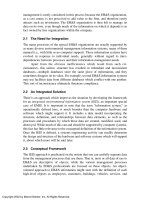
Heat and mass transfer coefficients are determined experimentally; the
results of such experiments are typically presented in terms of dimensionless
parameters. Table 3 lists a number of important dimensionless parameters. Thus,
heat transfer data are often presented in terms of the Nusselt number, Nu, a
dimensionless heat transfer coefficient. In many cases, the Nusselt number is
found to be a function of the Reynolds number Re and the Prandtl number Pr:
Nu = ƒ(Re,Pr) (63)
The equivalent relation for mass transfer is
Sh = ƒ(Re,Sc) (64)
where Sh is the Sherwood number and Sc is the Schmidt number (see Table 3).
Many standard handbooks and heat transfer textbooks list dimensionless transport
relationships for engineering systems (9,10).
4 STOICHIOMETRY AND CHEMICAL KINETICS
Stoichiometry is the study of the proportions in which elements combine to form
compounds. Chemical kinetics is the science dealing with the rates of chemical

reactions.
4.1 Stoichiometry
Consider a general chemical reaction in which reactants A, B, . . . react to form
products X, Z, . . . according to the equation
Copyright 2002 by Marcel Dekker, Inc. All Rights Reserved.
aA + bB + . . . = . . . + xX + zZ
This can be written in the equivalent form
0 =−aA − bB − . . . + xX + zZ
or, more compactly,
0 =
∑
k=1
n
ν
k
I
k
(65)
TABLE 3 Some Important Dimensionless Groups
Group Definition Significance
Nusselt number, Nu Nu≡
hL
k
Dimensionless heat
transfer coefficient
Péclet number, Pe
(thermal)
Pe ≡ Re ⋅ Pr Ratio of heat conduction
to convection
Péclet number, Pe

A
(chemical)
Pe
A
≡ Re ⋅ Sc
A
Ratio of species A diffu-
sion to convection
Prandtl number, Pr Pr ≡
µ/ρ
k/(ρC
^
p
)
=
µC
^
p
k
Ratio of momentum
transport to heat
conduction
Reynolds number, Re Re ≡
ρLν
µ
Ratio of inertial mo-
mentum transport to
viscous momentum
transport
Schmidt number, Sc

A
Sc
k
≡
µ/ρ
D
k
Ratio of viscous mo-
mentum transport to
species diffusion
Sherwood number, Sh
A
Sh
A
≡
k
A
L
D
A
Dimensionless mass
transfer coefficient for
species A
Notes:
C
^
p
≡ specific heat
D
i

≡ diffusivity of species i
h ≡ heat transfer coefficient
k
i
≡ mass transfer coefficient for species i
k ≡ thermal conductivity
L ≡ characteristic length
µ≡ viscosity
ρ≡ density
Copyright 2002 by Marcel Dekker, Inc. All Rights Reserved.
where ν
k
is the stoichiometric coefficient of species I
k
. Note that the stoichio-
metric coefficient is positive for a product and negative for a reactant.
4.2 Reaction Rate
The rate of a chemical reaction can be defined in terms of the stoichiometric
coefficient:
ξ
⋅
=
(N
⋅
A
)
gen
ν
A

=
(N
⋅
B
)
gen
ν
B

= . . . =
(N
⋅
k
)
gen
ν
k

= . . . =
(N
⋅
X
)
gen
ν
X

=
(N
⋅

Z
)
gen
ν
Z

(66)
Here, ξ is the extent of reaction variable or reaction coordinate. The volumetric
reaction rate r may be defined by:
r =
ξ
⋅
V
(67)
The volumetric reaction rate is usually a function of the temperature and
the concentrations of the various reactants and products:
r =±k(T)ƒ(c
A
,c
B
, . . . ,c
X
,c
Z
) (68)
where k(T) is the so-called rate constant (which is not really a constant, but rather
is a function of temperature).
In most cases, the rate constant is given by the Arrhenius equation:
k = k
0

exp



−E
a
RT



(69)
In this equation, k
0
is the preexponential factor and E
a
is the activation energy,
both of which must be determined experimentally.
The concentration-dependent part of the rate expression, ƒ(c
A
,c
B
, . . . , c
X
,
c
Z
, must also be determined experimentally. In many cases, the reaction rate is
found to depend on the concentrations of the reacting species as follows:
ƒ(c
A

,c
B
, . . .)=c
α
A
c
β
B
. . . (70)
A reaction that obeys this equation is said to be of “α order” in species A, of “β
order” in species B, and so on. The overall order of the reaction n is the sum of
the individual reaction orders:
n =α+β+ . . . (71)
More information on the determination of rate constants and their applica-
tions can be found in standard texts on kinetics and reactor design (6–8).
Copyright 2002 by Marcel Dekker, Inc. All Rights Reserved.
5 EQUILIBRIUM THERMODYNAMICS
Thermodynamics is the study of the relationship between heat, work, and various
forms of energy. Of particular interest to thermodynamics are the conditions for
equilibrium.
5.1 Auxiliary Thermodynamic Functions
In addition to the energy and entropy, it is common in thermodynamics to define
certain auxiliary functions. One of these is the enthalpy or heat function H:
H = U + PV (72)
Two common free-energy functions are defined. The Helmholtz free-energy
function A is defined by
A = U − TS (73)
The Gibbs free-energy function G is defined by
G = H − TS (74)
The Gibbs free-energy function is of special interest because it provides a

convenient criterion of spontaneity and equilibrium.
5.2 Spontaneity and Equilibrium
A spontaneous process is one that occurs in a closed system without the assistance
of some external agency. The Gibbs free energy decreases in a spontaneous
process:
∆G ≤ 0 (spontaneous process) (75)
At equilibrium, the system does not change with time. The Gibbs free energy
reaches a minimum at equilibrium:
dG
dt
= 0 (equilibrium) (76)
5.3 Fugacity
The change in Gibbs free energy for an ideal gas undergoing an isothermal
compression or expansion from pressure P
1
to pressure P
2
is given by
∆G = RT ln
P
2
P
1
(ideal gas) (77)
Although Eq. (77) does not apply for a real gas, it is common practice to retain
the same functional form for real gases:
Copyright 2002 by Marcel Dekker, Inc. All Rights Reserved.
∆G = RT ln
ƒ
2

ƒ
1
(real gas) (78)
Here, ƒ
1
is the fugacity at pressure P
1
. The fugacity may be considered as an
adjusted pressure. It is defined so as to coincide with the pressure at low densities:
lim
P→0
ƒ
P
= 1 (79)
The ratio of fugacity to pressure is called the fugacity coefficient, φ. Thus, the
previous equation may be written
ϕ≡
ƒ
P
⇒
lim
P→0
ϕ= 1 (80)
5.4 Chemical Potential
Consider a solution consisting of n species A, B, . . . . The Gibbs free energy of
the solution is given by
G =
∑
k=1
n

N
k
µ
k
(81)
where µ
k
is the chemical potential of species k, defined by
µ
k
=



∂G
∂N
k



T,P,N
j≠k
(82)
5.5 Fugacity and Activity
The chemical potential is generally a function of temperature, pressure, and
composition. It is common practice to write
µ
A
=µ˚
A

(T)+RT ln a
A
(83)
where µ˚
A
(T) is the standard chemical potential and a
A
is the activity of species
A. The activity is defined as the ratio of the fugacity ƒ
A
to a standard-state
fugacity ƒ˚
A
:
a
A
=
ƒ
A
ƒ˚
A
(84)
Activities and standard states are discussed in greater detail in many texts on
chemical thermodynamics (11,12).
Copyright 2002 by Marcel Dekker, Inc. All Rights Reserved.
5.6 Phase Equilibrium
Consider a multicomponent system that separates into two or more phases
(denoted I, II, . . .). The criteria for phase equilibrium are
T
I

= T
II
= . . . (thermal equilibrium) (85)
P
I
= P
II
= . . . (mechanical equilibrium) (86)
(µ
A
)
I
=(µ
A
)
II
= . . . (equilibrium for species A) (87)
(µ
B
)
I
=(µ
B
)
II
= . . . (equilibrium for species B) (88)
.
.
.
5.7 Reaction Equilibrium

Consider a reaction
aA + bB + . . . = . . . + xX + zZ
which, as before, can be expressed in the shorthand notation
0 =
∑
k=1
n
ν
k
I
k
The criterion for chemical reaction equilibrium is
∆G =
∑
k=1
n
ν
k
µ
k
= 0 (89)
Reaction equilibrium may also be expressed in terms of the standard Gibbs
free-energy change:
∆G
0
= RT ln K
a
(90)
Here, K
a

is the equilibrium constant, defined by
K
a
=
∏
k=1
n
a
k
ν
k
(91)
6 ENGINEERING FLUID MECHANICS
Fluid mechanics deals with the flow of liquids and gases. For most engineering
applications, a macroscopic approach is usually taken.
Copyright 2002 by Marcel Dekker, Inc. All Rights Reserved.
6.1 Engineering Bernoulli Equation
Most engineering problems in fluid mechanics can be solved using the engineer-
ing Bernoulli equation, also called the mechanical energy balance. It can be
derived from the macroscopic energy balance (see Ref. 13), subject to the
following restrictions: (a) the system is at steady state; (b) the system has a single
fluid intake and a single outlet; (c) gravity is the sole body force, with constant
|g|; (d) the flow is incompressible; (e) the system may include one or more pumps
or turbines. Under these conditions, the macroscopic energy balance becomes
∆



P
ρ

+ |g|z +
α
2
〈ν〉
2



=
W
⋅
s
m
⋅
−
F
⋅
m
⋅
(92)
where
P = the fluid pressure
〈ν〉 = the velocity averaged over the cross section of the pipe or conduit
α= average velocity correction factor (2.0 for laminar flow and 1.07 for
turbulent flow)
W
⋅
2
= rate of work done by pumps or turbines (positive for pumps,
negative for turbines)

F
⋅
= frictional loss rate
Dividing by the acceleration of gravity |g| yields the so-called head form of the
Bernoulli equation:
∆



P
ρ|g|
+ z +
α
2|g|
〈ν〉
2



=
W
⋅
s
m
⋅
|g|
−
F
⋅

m
⋅
|g|
(93)
Each of the terms in this equation has the dimensions of length.
6.2 Fluid Friction in Pipes and Conduits
The frictional loss rate F
⋅
equals the rate at which useful mechanical energy is
converted to thermal energy by friction. It is usually computed from an equation
of the form
F
⋅
m
⋅
= 4ƒ



L
D



〈ν〉
2
2
(94)
where ƒ is the Fanning friction factor.* In general, the friction factor is a function
*This is not the only friction factor in widespread use. Some authors prefer the Darcy-Wiessbach

friction factor, ƒ
DW
= 4ƒ.
Copyright 2002 by Marcel Dekker, Inc. All Rights Reserved.
of the pipe diameter D, the surface roughness ε, and the Reynolds number Re,
the latter being defined as
Re =
ρD|ν|
µ
(95)
where µ is the fluid viscosity.
In the laminar-flow regime, ƒ = 16/Re. For turbulent flows, a number of
charts, graphs, and equations are available to compute the friction factor. The
Colebrook equation has traditionally been used, although it requires a trial-and-
error solution to find ƒ:
1
√ƒ
=−4 log



ε/D
3.7
+
1.255
Re√ƒ



(96)

Wood’s approximation (Ref. 13) gives ƒ directly, without a trial-and-error
procedure:
ƒ = a + b Re
−c
(97)
where
a = 0.0235



ε
D



0.225
+ 0.1325



ε
D



(98)
b = 22




ε
D



0.44
(99)
c = 1.62



ε
D



0.134
(100)
The relations presented in this section were developed for cylindrical pipes or
tubes; however, the same equations may be used for noncylindrical ducts if the
pipe diameter D is replaced in Eqs. (94–100) by the hydraulic diameter D
H
:
D
H
= 4
volume of fluid
area wetted by fluid
(101)
6.3 Minor Losses

The relations developed in the previous section apply only to straight pipes or
conduits. Most pipelines, however, include bends, valves, and other fittings which
create additional frictional losses. These additional losses are often called “minor
losses,” although they may actually exceed the friction caused by the pipe itself.
There are two common ways to account for minor losses. One is to define
an equivalent length L
eq
which equals the length of straight pipe that would give
the same frictional loss as the valve or fitting in question. The total equivalent
Copyright 2002 by Marcel Dekker, Inc. All Rights Reserved.
length L
total
is the sum of the true length of the pipe and the individual equivalent
lengths of the valves and fitting:
L
total
= L
pipe
+
∑
fitting i
(L
eq
)
i
(102)
The total equivalent length L
total
is used in Eq. (94) in place of L to compute the
total frictional losses.

The second common approach to computing minor losses relies on the
concept of a loss coefficient K
L
, defined for each type of valve or fitting according
to the equation
F
⋅
m
⋅
= K
L
〈ν〉
2
2
(103)
A comprehensive listing of typical equivalent lengths and loss coefficients is
published by the Crane Company (14).
6.4 Fluid Friction in Porous Media
A porous medium is a solid material containing voids through which fluids may
flow. The most important single parameter used to described porous media is the
porosity or void fraction ε:
ε=
void volume
bulk volume
=
V
voids
V
voids
+ V

solid
(104)
Fluid friction in a porous medium of thickness L is usually described by Darcy’s law:
F
⋅
m
⋅
=
µ
ρ
L
k
〈ν〉 (105)
where k is a material property called the permeability.
REFERENCES
1. R. B. Bird, W. E. Stewart, and E. N. Lightfoot, Transport Phenomena. New York:
Wiley, 1960.
2. M. M. Denn, Process Fluid Mechanics. Englewood Cliffs, NJ: Prentice-Hall, 1980.
3. R. W. Fahien, Fundamentals of Transport Phenomena. New York: McGraw-Hill,
1983.
4. W. M. Deen, Analysis of Transport Phenomena. New York: Oxford University Press,
1998.
5. E. L. Cussler, Diffusion Mass Transfer in Fluid Systems, 2nd ed. Cambridge, U.K.:
Cambridge University Press, 1997.
Copyright 2002 by Marcel Dekker, Inc. All Rights Reserved.
6. O. Levenspiel, Chemical Reaction Engineering, 2nd ed. New York: Wiley, 1972.
7. H. S. Fogler, Elements of Chemical Reaction Engineering. Englewood Cliffs, NJ:
PTR Prentice-Hall, 1992.
8. L. D. Schmidt, The Engineering of Chemical Reactions. New York: Oxford Univer-
sity Press, 1998.

9. F. P. Incropera and D. P. DeWitt, Fundamentals of Heat and Mass Transfer, 3rd ed.
New York: Wiley, 1990.
10. D. R. Lide (ed.), CRC Handbook of Chemistry and Physics, 80th ed. Cleveland, OH:
CRC Press, 1999.
11. I. M. Klotz and R. M. Rosenberg. Chemical Thermodynamics: Basic Theory and
Methods, 3rd ed. Menlo Park, CA: W. A. Benjamin, 1972.
12. K. Denbigh, The Principles of Chemical Equilibrium, 3rd ed. Cambridge, U.K.:
Cambridge University Press, 1971.
13. N. De Nevers, Fluid Mechanics for Chemical Engineers, 2nd ed. New York:
McGraw-Hill, 1991.
14. Flow of Fluids Through Valves, Fittings, and Pipe, Crane Technical Paper 410.
Chicago: The Crane Company, 1988.
Copyright 2002 by Marcel Dekker, Inc. All Rights Reserved.