Mechanical Engineering Systems 2008 Part 7 pptx
Bạn đang xem bản rút gọn của tài liệu. Xem và tải ngay bản đầy đủ của tài liệu tại đây (442.05 KB, 25 trang )
Q
pP=
L
p=0
r R
142 Fluid mechanics
this effect is caused by the gravitational attraction between the two
planets but initially Newton thought that it was due to viscous drag in
the celestial fluid or ether that was held to fill the universe. When Venus
passed the earth it would shear this fluid in the relatively small gap
between the two planets and there would be a resistance or drag force
which would act to slow Venus down while speeding up the earth.
Newton pursued this theory to the point of tabletop experiments with
liquids and plates and produced an equation which basically describes
and defines viscosity, before discarding the idea in favour of gravity.
The equation that Newton developed to define the viscosity of a fluid
is:
Viscous shear stress = viscosity × velocity gradient
In its simplest form this can be applied to two flat plates, one moving
and one stationary, in the following equation:
F
A
=
u
h
(3.2.4)
Here the force F applied to one of the plates, each of area A and
separated by a gap of width h filled with fluid of viscosity , produces
a difference in velocity of u. The viscosity is correctly known as the
dynamic viscosity and has the units of Pascal seconds (Pa s). These are
identical to N s/m
2
and kg/m/s.
For the case where these two plates are adjacent lamina or layers:
F = A × velocity gradient
We have replaced the term u/h with something called the velocity
gradient which will allow us later to apply Newton’s equation to
situations where the velocity does not change evenly across a gap.
We can apply this to pipe flow if we now wrap the lamina into
cylinders.
Laminar flow in pipes (Figure 3.2.10)
We said earlier that most fluid flow applications of interest to mechanical
engineers involve turbulent flow, but there are some increasingly
important examples of laminar flow where the pipe diameter is small and
the liquid is very viscous. The field of medical engineering has many such
examples, such as the flow of viscous blood along the small diameter
tubes of a kidney dialysis machine. It is therefore necessary for us to study
this kind of pipe flow so that we may be able to calculate the pumping
pressure required to operate this type of device.
Consider flow at a volume flow rate Q m
3
/s along a pipe of radius R and
length L. The liquid viscosity is and a pressure drop of P is required
across the ends of the pipe to produce the flow. Let us look at the forces on
the cylindrical core of the liquid in the pipe, up to a radius of r.
If we take the outlet pressure as 0 and the inlet pressure as P then the
force pushing the core to the right, the pressure force, is given by
F
p
= P × A
= r
2
P
Figure 3.2.10 Laminar flow
along a pipe
Fluid mechanics 143
The force resisting this movement is the viscous drag around the
cylindrical surface of the core. Using Newton’s defining equation for
viscosity, Equation (3.2.4),
F
drag
= A
core surface
× velocity gradient
= 2 rL
dv
dr
For steady flow these forces must be equal and opposite,
F
p
= –F
drag
r
2
P = –2r L
dv
dr
rP = –2L
dv
dr
So the velocity gradient is
dv
dr
= –
rP
2L
This is negative because v is a maximum at the centre and decreases
with radius.
We need to relate the pressure to the flow rate Q and the first step is
to find the velocity v at any radius r by integration.
v =
͵
–
rP
2L
dr
= –
r
2
P
4L
+ C
To evaluate the constant C we note that the liquid is at rest (v = 0) at the
pipe wall (r = R). Even for liquids which are not sticky or highly
viscous, all the experimental evidence points to the fact that the last
layer of molecules close to the walls fastens on so tightly that it does not
slip (Figure 3.2.11).
Therefore
0=–
R
2
P
4L
+ C, so C =
R
2
P
4L
Therefore
v =
P
4L
(R
2
– r
2
)
Figure 3.2.11 Velocity
distribution inside the pipe
144 Fluid mechanics
This is the equation of a parabola so the average or mean velocity
equals half the maximum velocity, which is on the central axis.
v
mean
=
1
2
V
axis
Now volume flow rate is Q = V
mean
× area.
This is the continuity equation and up to now we have only applied
it to turbulent flow where all the liquid flows at the same velocity and
we do not have to think of a mean. So
Q =
V
axis
2
R
2
Finally
Q =
PR
4
8L
(3.2.5)
This is called Poiseuille’s law after the French scientist and engineer who
first described it and this type of flow is known as Poiseuille flow.
Note that this is analogous to Ohm’s law with flow rate Q equivalent
to current I, pressure drop P equivalent to voltage E and the term
8L
R
4
representing fluid resistance ⍀, equivalent to resistance R.
Hence Ohm’s law E = IR becomes P = Q⍀ when applied to viscous
flow along pipes. This can be very useful when analysing laminar flow
through networks of pipes. For example, the combined fluid resistance
of two different diameter pipes in parallel and both fed with the same
liquid at the same pressure can be found just like finding the resistance
of two electrical resistors in parallel.
Example 3.2.3
A pipe of length 10 m and diameter 5 mm is connected in
series to a pipe of length 8 m and diameter 3 mm. A pressure
drop of 120 kPa is recorded across the pipe combination
when an oil of viscosity 0.15 Pa s flows through it. Calculate
the flow rate.
First we must calculate the two fluid resistances, one for
each section of the pipe.
⍀
1
=8 × 10 × 0.15/(0.0025
4
) = 9.778 × 10
10
Pa s/m
3
⍀
1
=8 × 8 × 0.15/(0.0015
4
) = 60.361 × 10
10
Pa s/m
3
Total resistance = 70.139 × 10
10
Pa s/m
3
The flow rate is then given by:
Q = P/⍀ = 120 000/70.139 × 10
10
Pa s/m
3
= 1.71 × 10
–7
m
3
/s
Z
1
A
1
V
1
1
2
Z
2
A
2
P
2
V
2
P
1
Datum level
Fluid mechanics 145
Examples of laminar flow in engineering
We have already touched on one example of laminar flow in pipes
which is highly relevant to engineering but it is worthwhile looking at
some others just to emphasize that, although turbulent flow is the more
important, there are many instances where knowledge of laminar flow is
necessary.
One example from mainstream mechanical engineering is the
dashpot. This is a device which is used to damp out any mechanical
vibration or to cushion an impact. A piston is pushed into a close-fitting
cylinder containing oil, causing the oil to flow back along the gap
between the piston and the cylinder wall. As the gap is small and the oil
has a high viscosity, the flow is laminar and the pressure drop can be
predicted using an adaptation of Poiseuille’s law.
A second example which is more forward looking is from the field of
micro-fluidics. Silicon chip technology has advanced to the point where
scientists can build a small patch which could be stuck on a diabetic’s
arm to provide just the right amount of insulin throughout the day. It
works by drawing a tiny amount of blood from the arm with a miniature
pump, analysing it to determine what dose of insulin is required and
then pumping the dosed blood back into the arm. The size of the flow
channels is so small, a few tens of microns across, that the flow is very
laminar and therefore so smooth that engineers have had to go to great
lengths to ensure effective mixing of the insulin with the blood.
Conservation of energy
Probably the most important aspect of engineering is the energy
associated with any application. We are all painfully aware of the cost
of energy, in environmental terms as well as in simple economic terms.
We therefore now need to consider how to keep account of the energy
associated with a flowing liquid. The principle that applies here is the
law of conservation of energy which states that energy can neither be
created nor destroyed, only transferred from one form to another. You
have probably met this before, and so we have a fairly straightforward
task in applying it to the flow of liquids along pipes. If we can calculate
the energy of a flowing liquid at the start of a pipe system, then we know
that the same total of energy must apply at the end of the system even
though the values for each form of energy may have altered. The only
problem is that we do not know at the moment how to calculate the
energy associated with a flowing liquid or even how many types of
energy we need to consider. We must begin this calculation therefore by
examining the different forms of energy that a flowing liquid can have
(Figure 3.2.12).
Figure 3.2.12 Energy of a
flowing liquid
146 Fluid mechanics
If we ignore chemical energy and thermal energy for the purposes of
flow calculations, then we are left with potential energy due to height,
potential energy due to pressure and kinetic energy due to the motion.
In Figure 3.2.12 adding up all three forms of energy at point 1 for a
small volume of liquid of mass m:
Potential energy due to height is calculated with reference to some
datum level, such as the ground, in the same way as for a solid.
PE
height
= mgz
1
Potential energy due to pressure is a calculation of the fact that the
mass m could rise even higher if the pipe were to spring a leak at point
1. It would rise by a height of h
1
equal to the height of the liquid in a
manometer tube placed at point 1, where h
1
is given by h
1
= p
1
/g.
Therefore the energy due to the pressure is again calculated like the
height energy of a solid.
PE
pressure
= mgh
1
Note that the height h
1
is best referred to as a pressure head in order to
distinguish it from the physical height z
1
of the pipe at this point.
Kinetic energy is calculated in the same way as for a solid.
KE =
1
2
mv
1
2
Therefore the total energy of the mass m at point 1 is given by
E
1
= mgz
1
+ mgh
1
+
1
2
mv
1
2
Similarly the energy of the same mass at point 2 is given by
E
2
= mgz
2
+ mgh
2
+
1
2
mv
2
2
From the principle of conservation of energy we know that these two
values of the total energy must be the same, provided that we can ignore
any losses due to friction against the pipe wall or within the liquid.
Therefore if we cancel the m and divide through by g, we produce the
following equation:
z
1
+ h
1
+ v
1
2
/2g = z
2
+ h
2
+ v
2
2
/2g (3.2.6)
This is known as Bernoulli’s equation after the French scientist who
developed it and is the fundamental equation of hydrodynamics. The
dimensions of each of the three terms are length and therefore they all
have units of metres. For this reason the third term, representing kinetic
energy, is often referred to as the velocity head, in order to use the
familiar concept of head which already appears as the second term on
both sides of the equation. The three terms on each side of the equation,
added together, are sometimes known as the total head. A second
advantage to dividing by the mass m and eliminating it from the
equation is that we no longer have to face the problem that it would be
very difficult to keep track of that fixed mass of liquid as it flowed along
the pipe. Turbulent flow and laminar flow would both make the mass
spread out very rapidly after the starting point.
Paint
Paint/ai
r
spray
Air
Air
Fuel/air mixture
Fuel
Fluid mechanics 147
Bernoulli’s equation describes the fact that the total energy in an ideal
flowing liquid stays constant between two points. It is very much a
practical engineering equation and for this reason it is commonly
reduced to the form given here where all the terms are measured in
metres. A pipeline designer, for example, could use it to keep track of
how the pressure head would change along a pipe system as it followed
the local terrain over hill and valley, without any need to ever work in
joules, the true units of energy.
When carrying out calculations on Bernoulli’s equation it is
sometimes useful to use the substitution h = p/g to change from head
to pressure, and it is often useful to use the substitution v = Q/A because
the volume flow rate is the most common way of describing the liquid’s
speed.
An example of the use of Bernoulli’s equation is given later in
Example 3.2.5.
Venturi principle
Bernoulli’s equation can seem very daunting at first sight, but it is
worthwhile remembering that it is simply the familiar conservation of
energy principle. Therefore it is not always necessary to put numbers
into the equation in order to predict what will happen in a given flow
situation. One of the most useful applications in this respect is the
behaviour of the fluid pressure when the fluid, either liquid or gas, is
made to go through a constriction.
Consider what happens in Figures 3.2.13 and 3.2.14
In both cases the fluid, air, is pushed through a narrower diameter
pipe by the high pressure in the large inlet pipe. The velocity in the
narrow pipe is increased according to the relationship v = Q/A since the
volume flow rate Q must stay constant. Hence the kinetic energy term
v
2
/2g in Bernoulli’s equation is greatly increased, and so the pressure
head term h or p/g must be much reduced if we can ignore the change
in physical height over such a small device. The result is that a very low
pressure is observed at the narrow pipe, which can be used to suck paint
in through a side pipe in the case of the spray gun in Figure 3.2.13, or
petrol in the case of the carburettor in Figure 3.2.14. This effect is
known as the Venturi principle after the Italian scientist and engineer
who discovered it.
Measurement of fluid flow
Fluid mechanics for the mechanical engineer is largely concerned
with transporting liquid from one place to another and therefore it is
important that we have an understanding of some of the ways of
measuring flow. There are many flow measurement methods, some of
which can be used for measuring volume flow rates, others which
can be used for measuring flow velocity, and yet others which can be
used to measure both. We shall limit ourselves to analysis of one
example of a simple flow rate device and one example of a velocity
device.
Figure 3.2.13 Paint sprayer
Figure 3.2.14 Carburettor
Inlet Inlet cone
Throat Diffuser
hh
12
–
148 Fluid mechanics
Measurement of volume flow rate – the Venturi
meter
In the treatment of Bernoulli’s equation we found that changing the
velocity of a fluid through a change of cross-section leads to a change
in the pressure as the total head remains constant. In the Venturi effect
the large increase in velocity through a constriction causes a marked
reduction in pressure, with the size of this reduction depending on the
size of the velocity increase and therefore on the degree of constriction.
In other words, if we made a device which forced liquid through a
constriction and we measured the pressure head reduction at the
constriction, then we could use this measurement to calculate the
velocity or the flow rate from Bernoulli’s equation.
Such a device is called a Venturi meter since it relies on the Venturi
effect. In principle the constriction could be an abrupt change of
cross-section, but it is better to use a more gradual constriction and an
even more gradual return to the full flow area following the
constriction. This leads to the formation of fewer eddies and smaller
areas of recirculating flow. As we shall see later, this leads to less loss
of energy in the form of frictional heat and so the device creates less
of a load to the pump producing the flow. A typical Venturi meter is
shown in Figure 3.2.15.
The inlet cone has a half angle of about 45° to produce a flow pattern
which is almost free of recirculation. Making the cone shallower would
produce little extra benefit while making the device unnecessarily
long.
The diffuser has a half angle of about 8° since any larger angle leads
to separation of the flow pattern from the walls, resulting in the
formation of a jet of liquid along the centreline, surrounded by
recirculation zones.
The throat is a carefully machined cylindrical section with a smaller
diameter giving an area reduction of about 60%.
Measurement of the drop in pressure at the throat can be made using
any type of pressure sensing device but, for simplicity, we shall consider
the manometer tubes shown. The holes for the manometer tubes – the
pressure taps – must be drilled into the meter carefully so that they are
accurately perpendicular to the flow and free of any burrs.
Figure 3.2.15 A typical Venturi
meter
Fluid mechanics 149
Analysis of the Venturi meter
The starting point for the analysis is Bernoulli’s equation:
z
1
+ h
1
+ v
1
2
/2g = z
2
+ h
2
+ v
2
2
/2g
Since the meter is being used in a horizontal position, which is the usual
case, the two values of height z are identical and we can cancel them
from the equation.
h
1
+ v
1
2
/2g = h
2
+ v
2
2
/2g
The constriction will cause some non-uniformity in the velocity of the
liquid even though we have gone to the trouble of making the change in
cross-section gradual. Therefore we cannot really hope to calculate the
velocity accurately. Nevertheless we can think in terms of an average or
mean velocity defined by the familiar expression:
v = Q/a
Therefore, remembering that the volume flow rate Q does not alter
along the pipe:
h
1
+ Q
2
/2a
1
2
g = h
2
+ Q
2
/2a
2
2
g
We are trying to get an expression for the flow rate Q since that is what
the instrument is used to measure, so we need to gather all the terms
with it onto the left-hand side:
(Q
2
/2g) × (1/a
1
2
– 1/a
2
2
)=h
2
– h
1
Q
2
=2g(h
2
– h
1
)/(1/a
1
2
– 1/a
2
2
)
Since h
1
> h
2
it makes sense to reverse the order in the first set of
brackets, compensating by reversing the order in the second set as
well:
Q
2
=2g(h
1
– h
2
)/(1/a
2
2
– 1/a
1
2
)
Finally we have:
Q =
ͱ{2g(h
1
– h
2
)/(1/a
2
2
– 1/a
1
2
)} (3.2.7)
This expression tells us the volume flow rate if we can assume that
Bernoulli’s equation can be applied without any consideration of head
loss, or energy loss, in the device. In practice there will always be losses
of energy, and head, no matter how well we have guided the flow
through the constriction. We could experimentally measure a head loss
and use this in a modified form of Bernoulli’s equation, but it is
customary to stick with the analysis carried out above and make a final
correction at the end.
Any loss of head will lead to the drop in heights of manometer levels
across the meter being bigger than it should be ideally. Therefore the
calculated flow rate will be too large and so it must be corrected by
Orifice
150 Fluid mechanics
applying some factor which makes it smaller. This factor is known as
the discharge coefficient C
D
and is defined by:
Q
real
= C
D
× Q
ideal
In a well-manufactured Venturi meter the energy losses are very small
and so C
D
is very close to 1 (usually about 0.97).
In some situations it would not matter if the energy losses caused by
the flow measuring device were considerably higher. For example, if
you wanted to measure the flow rate of water entering a factory then
even a considerable energy loss caused by the measurement would only
result in the pumps at the local water pumping station having to work a
little harder; there would be no disadvantage as far as the factory was
concerned. In these circumstances it is not necessary to go to the trouble
of having a carefully machined, highly polished Venturi meter,
particularly since they are complicated to install. Instead it is sufficient
just to insert an orifice plate at any convenient joint in the pipe,
producing a device known as an Orifice meter (Figure 3.2.16). The
orifice plate is rather like a large washer with the central hole, or orifice,
having the same sort of area as the throat in the Venturi meter.
The liquid flow takes up a very similar pattern to that in the Venturi
meter, but with the addition of large areas of recirculation. In particular
the flow emerging from the orifice continues to occupy a small cross-
section for quite some distance downstream, leading to a kind of throat.
The analysis is therefore identical to that for the Venturi meter, but the
value of the discharge coefficient C
D
is much smaller (typically about
0.6). Since there is not really a throat, it is difficult to specify exactly
where the downstream pressure tapping should be located to get the
most reliable reading, but guidelines for this are given in a British
Standard.
Measurement of velocity – the Pitot-static tube
Generally it is the volume flow rate which is the most important
quantity to be measured and from this it is possible to calculate a mean
flow velocity across the full flow area, but in some cases it is also
important to know the velocity at a point. A good example of this is in
a river where it is essential for the captain of a boat to know what
Figure 3.2.16 An orifice meter
V
90° bend
Glass tube
h
h
Bucket
Pitot tube
Static tube
Inlet
f
or Pitot
tube
Inlets for static tube
Inner
Pitot tube
Outer
static tube
Fluid mechanics 151
strength of current to expect at any given distance from the bank;
calculating a mean velocity from the volume flow rate would not be
much help even if it were possible to measure the exact flow area over
an uneven river bed.
It was exactly this problem which led to one of the most common
velocity measurement devices. A French engineer called Pitot was given
the task of measuring the flow of the River Seine around Paris and
found that a quick and reliable method could be developed from some
of the principles we have already met in the treatment of Bernoulli’s
equation. Figure 3.2.17 shows the early form of Pitot’s device.
The horizontal part of the glass tube is pointed upstream to face the
oncoming liquid. The liquid is therefore forced into the tube by the
current so that the level rises above the river level (if the glass tube was
simply a straight, vertical tube then the water would enter and rise until
it reached the same level as the surrounding river). Once the water has
reached this higher level it comes to rest.
What is happening here is that the velocity head (kinetic energy) of
the flowing water is being converted to height (potential energy) inside
the tube as the water comes to rest. The excess height of the column of
water above the river level is therefore equal to the velocity head of the
flowing water:
h = v
2
/2 g
Therefore the velocity measured by a Pitot tube is given by:
v =
ͱ(2gh) (3.2.7)
In practice Pitot found it difficult to note the level of the water in the
glass tube compared to the level of the surrounding water because of the
disturbances on the surface of the river. He quickly came up with the
practical improvement of using a straight second tube (known as a static
tube) to measure the river level because the capillary action in the
narrow tube damped down the fluctuations (Figure 3.2.18).
The Pitot-static tube is still widely used today, most notably as the
speed measurement device on aircraft (Figure 3.2.19).
The two tubes are now combined to make them co-axial for the
purposes of ‘streamlining’, and the pressure difference would be
Figure 3.2.17 The Pitot tube
Figure 3.2.18 An early Pitot-
static tube
Figure 3.2.19 A modern Pitot-
static tube
152 Fluid mechanics
measured by an electronic transducer, but essentially the device is the
same as Pitot’s original invention. Because the Pitot tube and the static
tube are united, the device is called a Pitot-static tube.
Example 3.2.4
A Pitot-static tube is being used to measure the flow velocity
of liquid along a pipe. Calculate this velocity when the heights
of the liquid in the Pitot tube and the static tube are 450 mm
and 321 mm respectively.
The first thing to do is calculate the manometric head
difference, i.e. the difference in reading between the two
tubes.
Head difference = 450 mm – 321 mm = 129 mm
= 0.129 m
Then use Equation (3.2.7),
Velocity =
ͱ(2 × 9.81 × 0.129) = 1.59 m/s
Losses of energy in real fluids
So far we have looked at the application of the familiar ‘conservation of
energy’ principle to liquids flowing along pipes and developed
Bernoulli’s equation for an ideal liquid flowing along an ideal pipe.
Since energy can neither be created nor destroyed, it follows that the
three forms of energy associated with flowing liquids – height energy,
pressure energy and kinetic energy – must add up to a constant amount
even though individually they may vary. We have used this concept to
understand the working of a Venturi meter and recognized that a
practical device must somehow take into account the loss of energy
from the fluid in the form of heat due to friction. This was quite simple
for the Venturi meter as the loss of energy is small but we must now
consider how we can take into account any losses in energy, in the form
of heat, caused by friction in a more general way. These losses can arise
in many ways but they are all caused by friction within the liquid or
friction between the liquid and the components of the piping system.
The big problem is how to include what is essentially a thermal effect
into a picture of liquid energy which deliberately sets out to exclude any
mention of thermal energy.
Modified Bernoulli’s equation
Bernoulli’s equation, as developed previously, may be stated in the
following form:
z
1
+ h
1
+ v
1
2
/2 g = z
2
+ h
2
+ v
2
2
/2 g
All the three terms on each side of Bernoulli’s equation have dimensions
of length and are therefore expressed in metres. For this reason the total
value of the three terms on the left-hand side of the equation is known
Fluid mechanics 153
as the initial total head in just the same way as we used the word head
to describe the height h associated with any pressure p through the
expression
p = gh
Similarly the right-hand side of the equation is known as the final total
head. Bernoulli’s equation for an ideal situation may also be expressed
in words as:
Initial total head = final total head
What happens when there is a loss of energy due to friction with a real
fluid flowing along a real pipe is that the final total head is smaller than
the initial total head. The loss of energy, as heat generated by the friction
and dissipated through the liquid and the pipe wall to the surroundings,
can therefore be expressed as a loss of head. Note that we are not
destroying this energy, it is just being transformed into thermal energy
that cannot be recovered into a useful form again. As far as the engineer
in charge of the installation is concerned this represents a definite loss
which needs to be calculated even if it cannot be reduced any further.
What happens in practice is that manufacturers of pipe system
components, such as valves or couplings, will measure this loss of head
for all their products over a wide range of sizes and flow rates. They will
then publish this data and make it available to the major users of the
components. Provided that the sum of the head losses of all the
components in a proposed pipe system remains small compared to the
total initial head (say about 10%) then it can be incorporated into a
modified Bernoulli’s equation as follows:
Initial total head – head losses = final total head
With this equation it is now possible to calculate the outlet velocity or
pressure in a pipe, based on the entry conditions and knowledge of the
energy losses expressed as a head loss in metres. Once again we see the
usefulness of working in metres since engineers can quickly develop a
feel for what head loss might be expected for any type of fitting and how
it could be compensated. This would be extremely difficult to do if
working in conventional energy units.
Example 3.2.5
Water is flowing downwards along a pipe at a rate of 0.8 m
3
/s
from point A, where the pipe has a diameter of 1.2 m, to point
B, where the diameter is 0.6 m. Point B is lower than point A
by 3.3 m. The pipe and fittings give rise to a head loss of
0.8 m. Calculate the pressure at point B if the pressure at
point A is 75 kPa (Figure 3.2.20).
Since the information in the question gives the flow rate Q
rather than the velocities, we shall use the substitution
Q = a
1
v
1
= a
2
v
2
A
B
Q
3.3 m
Q = 0.8m /s
3
Q
E
nergy
l
oss reg
i
ons
154 Fluid mechanics
Therefore the modified Bernoulli’s equation becomes:
z
1
+ p
1
/g + Q
2
/2a
1
2
g – losses = z
2
+ p
2
/g + Q
2
/2a
2
2
g
The absolute heights of point A and point B do not matter, it
is only the relative difference in heights which is important.
Therefore we can put z
1
= 3.3 m and z
2
= 0
3.3 + 75 000/(1000 × 9.81) + 0.8
2
/(2 × ( × 0.6
2
)
2
× 9.81) – 0.8
=0 + p
2
/(1000 × 9.81) + 0.8
2
/(2 × ( × 0.3
2
)
2
× 9.81)
3.3 + 7.645 + 0.0255 – 0.8 = 0 + p
2
/9810 + 0.4080
10.71 = p
2
/9810 + 0.4080
Therefore:
p
2
= 9810 × (10.71 – 0.4080)
= 101.1 kPa
The cause of energy losses
Earlier we looked at the way that liquids flow along pipes and we
showed that almost all practical cases involved turbulent flow where the
liquid molecules continually collide with each other and with the walls.
It is the collisions with the walls which transfer energy from the liquid
to the surroundings; the molecules hit a roughness point on the wall and
lose some of their kinetic energy as a tiny amount of localized heating
of the material in the pipe wall.
The molecules therefore bounce off the walls with slightly lower
velocity, but this is rapidly restored to its original value in collisions
with other molecules. If this velocity remained lower following a
collision then the liquid would not flow along the pipe at the proper rate.
This cannot happen since it would violate the continuity law, which
states that the flow rate must remain constant. In fact the energy to keep
the molecules moving at their original speed following a collision with
the wall comes from the pressure energy, which is why the effect of
friction appears as a loss of head.
Losses in pipe fittings
Let us look at a typical pipe fitting to see where the energy loss arises
(see Figure 3.2.21).
Figure 3.2.20 A pipe system with energy losses
Figure 3.2.21 Flow patterns
through a typical pipe fitting
Q
Fluid mechanics 155
The sudden contraction of the flow caused by joining two pipes of
different diameters gives rise to regions of recirculating flow or eddies.
The liquid which enters these regions is trapped and becomes separated
from the rest of the flow. It goes round and round, repeatedly hitting the
pipe walls and losing kinetic energy, only to be restored to its original
speed by robbing the bulk flow of some of its pressure energy. The
energy is dissipated as heat through the pipe walls. If the overall
pressure drop was critical and the head loss needed to be kept to a
minimum, then a purpose-built pipe fitting could be designed to connect
the two pipes with much less recirculation. Essentially this would round
off the sharp corners (Figure 3.2.22).
Since it is kinetic energy which is lost in the collisions which are a
feature of recirculating eddies, it follows that faster liquids will lose
more energy than slower liquids in the same situation. In extensive
experiments it has been found that the energy loss in fact depends on the
overall kinetic energy of the liquid as it meets the obstruction. The
proportion of the kinetic energy that is lost is approximately a constant
for any given shape of obstruction, such as a valve or a pipe fitting,
irrespective of the size.
For the purposes of calculations involving Bernoulli’s equation it is
convenient to work in terms of the velocity head (i.e. the third term
v
2
/2 g in Bernoulli’s equation) when considering kinetic energy.
Therefore a head loss for a particular type of pipe fitting is usually
expressed as:
Head loss = loss coefficient × velocity head
h
loss
= k × (v
2
/2 g) (3.2.8)
Some typical values of k are shown below, but it must be remembered
that they are only approximate.
Approximate loss coefficient k for some typical
pipe fittings
90° threaded elbow 0.9
90° mitred elbow 1.1
45° threaded elbow 0.4
Globe valve, fully open 10
Gate valve,
fully open 0.2
3/4 open 1.15
1/2 open 5.6
1/4 open 24
Turbulent flow in pipes – frictional losses
One of the basic things that engineers need to know when designing and
building anything involving flow of fluids along pipes is the amount of
energy lost due to friction for a given pipe system at a given flow rate.
Figure 3.2.22 Flow patterns
through a streamlined pipe
fitting
156 Fluid mechanics
We have just looked at the losses in individual fittings as these are of most
importance in a short pipe system, such as would be found in the fuel or
hydraulic system in a car. Increasingly, however, mechanical engineers
are becoming involved in the design of much larger pipe systems such as
would be found in a chemical plant or an oil pipeline. For these pipe
lengths the head loss due to friction becomes appreciable for the pipes
themselves, even though modern pipes are seemingly very smooth.
The energy loss due to friction appears as a loss of pressure
(remember pressure and kinetic energy are the two important forms of
energy for flow along a horizontal pipe – loss of kinetic energy becomes
transformed into a loss of pressure). Therefore if we use simple
manometers to record the pressure head along a pipeline then we
observe a gradual loss of head. The slope of the manometer levels is
known as the hydraulic gradient (Figure 3.2.23).
The head reading on the manometers can be held constant if the pipe
itself goes downhill with a slope equal to the hydraulic gradient. Of
course we do not really need to install manometer tubes every few
metres; we can simply calculate the total head at any point and keep
track of its gradual reduction mathematically.
There is no way of predicting the loss of head completely analytically
and so we rely on an empirical law based on the results of a large
number of experiments carried out by a French engineer Henri Darcy
(or d’Arcy) in the nineteenth century. His results for turbulent flow were
summed up as follows:
h
f
=
4fL
d
v
2
2 g
(3.2.9)
where:
h
f
= head loss due to friction (m)
v = flow velocity (m/s)
L = pipe length (m)
d = pipe diameter (m)
f = friction factor (no units).
Intuitively we can see where each of these terms comes from in the
overall equation, as follows:
᭹ The frictional head loss clearly depends on the length of the pipe, L,
as we would expect a pipe that is twice as long to have a head loss
that is also twice as great.
Figure 3.2.23 Hydraulic
gradient
0.025
0.020
0.015
0.010
0.009
0.008
0.007
0.006
0.005
0.004
0.003
0.002
Friction factor
Re
y
nolds number
Turbulent flow
Turbulent flow
Smooth pipes
Smooth pipes
10
3
234568
10
4
10
5
10
6
10
7
222333444555666888
10
8
10
8
2
2
3
3
4
4
5
5
6
6
8
8
– 0.00001
0.00005
Laminar flow
Laminar flow
Relative roughness
0.0001
0.0002
0.0004
0.0006
0.0008
0.001
0.002
0.004
0.006
0.008
0.01
0.015
0.02
0.03
0.04
0.05
0.000 00
5
0.000 001
Fluid mechanics 157
᭹ Head loss decreases with increasing pipe diameter because a smaller
proportion of the liquid comes into contact with the pipe wall.
᭹ Friction arises from loss of kinetic energy and so the expression
must have velocity head (V
2
/2 g) in it (which is why we do not
cancel the 2 and the 4).
᭹ Head loss also depends on the resistance offered by the roughness
of the pipe wall, as represented by the friction factor f.
The friction factor is generally quoted by a pipe manufacturer. It
depends on the material and the type of production process (both of
which affect the roughness), on the diameter and the flow velocity, and
on the amount of turbulence (Reynolds number).
D’Arcy’s equation was used successfully for almost 100 years,
relying on values of the friction coefficient f that were found
experimentally for the very few types of pipes that were available and
mostly for gravity feed systems. Once pumping stations and standard-
ized pipes came into common use, however, a more accurate estimate of
head loss at the much higher flow rates was required. It became apparent
that the friction coefficient f varied quite considerably with type of pipe,
diameter, flow rate, type of liquid, etc. The problem was solved by an
American engineer called Moody who carried out a vast number of
experiments on as many combinations of pipes and liquids as he could
find. He assembled all the experimental data into a special chart, now
called a Moody chart, as shown in Figure 3.2.24.
This has a series of lines on a double logarithmic scale. Each line
corresponds to a pipe of a given ‘relative roughness’ and is drawn on
axes which represent friction factor and Reynolds number. To
Figure 3.2.24 Moody chart
158 Fluid mechanics
understand the chart we must first look at the pipe roughness as this is
the parameter which gives rise to most of the friction.
The roughness on the inside of the pipe is firstly expressed as an
‘equivalent height’ of roughness. This is an averaging process which
imagines the actual randomly scattered roughness points being replaced
by a series of identical rough points, all of one height, which produce
the same effect. The pipe manufacturers will produce this information
using a surface measurement probe linked to a computer. This
equivalent roughness height K is then divided by the pipe diameter d to
give the relative roughness, K/d, plotted down the right-hand edge of the
chart. Note that the relative roughness has no units, it is simply a ratio.
Therefore the whole chart is dimensionless since the axes themselves
are friction factor and Reynolds number, neither of which has units.
To use the chart, calculate the relative roughness if it is not given, and
then locate the nearest line (or lines) at the right-hand edge. Be prepared
to estimate values between the curves. Then move to the left along the
curve until the specified value of Reynolds number Re is reached along
the bottom edge. If the flow is turbulent (Re > 2–4000) then it is
possible to read off the value of friction factor f corresponding to where
the experimental line cuts the Re line. This value is then used in
d’Arcy’s equation. For example,
For relative roughness = 0.003 and Re = 1.3 × 10
5
, f = 0.0068
Notes on the Moody chart
(1) The shaded region is for transitional flows, neither fully turbulent
nor fully laminar, so generally the worst case is assumed, i.e. the
highest value of friction factor is taken.
(2) For laminar flow:
h
f
=
4fL
d
V
2
2 g
so the pressure drop is given by
P = g ·
4fL
d
·
V
2
2 g
Using Q = VA = Vd
2
/4,
P =
8fLv
d
3
Q =
8fL·Re
d
4
Q
Comparing this with Poiseuille’s law,
P =
8 L
R
4
Q
and noting that
d
4
= 16R
4
Then
f =
16
Re
This is the straight line on the left of the chart.
High
velocity
water jet
Low velocity
water input
Hose
Nozzle
Fluid mechanics 159
This is an artificial use of friction factor because the pressure drop in
laminar flow is really directly proportional to V, whereas in turbulent
flow it is proportional to V
2
(i.e. kinetic energy).
Nevertheless, the laminar flow line is included on the Moody chart so
that the design engineer can quickly move from the common turbulent
situations to the less frequent applications where the flow rate is small
and the product in the pipeline is very viscous. If the pressure drop along
a pipe containing laminar flow is required then normally Poiseuille’s
equation would be used.
The momentum principle
This section deals with the forces associated with jets of fluid and
therefore has applications to jet engines, turbines and compressors. It is
an application of Newton’s second law which is concerned with
acceleration. Since acceleration covers changes of direction as well as
changes of speed, the forces on pipe bends due to the fluid turning
corners is also covered. As usual we shall concentrate on liquids for the
sake of simplicity.
When a jet of liquid is produced, for example from a fire hose as
shown in Figure 3.2.25, it is given a large velocity by the action of the
nozzle; the continuity law means that the liquid has to go faster to pass
through the small cross-section at the same flow rate. The idea behind
giving it this large velocity in this case is to allow the jet of water to
reach up into tall buildings.
In the short time it takes to flow along the nozzle the liquid therefore
receives a great deal of momentum. According to Newton’s second law
of motion, the rate of change of this momentum is equal to the force
which must be acting on the liquid to make it accelerate. Similarly from
Newton’s third law there will be a reaction force on the hose itself. That
is why it usually takes two burly fire fighters to hold a hose and point
it accurately when it is operating at full blast.
At the other end of the jet there is a similar change of momentum as
the jet is slowed down when it hits a solid object. Again this can be a
considerable force; in some countries the riot police are equipped with
water cannon which project a high velocity water jet to knock people off
their feet!
Calculation of momentum forces
To calculate the forces associated with jets we must go back to
Newton’s original definition of forces in order to see how liquids differ
from solids.
What Newton stated was that the force on an accelerating body was
equal to the rate of change of the body’s momentum.
Force = rate of change of momentum
F = d/dt (mv)
For a solid this differentiation is straightforward because the mass m is
usually constant. Therefore we get:
F = m dv/dt
Figure 3.2.25 Fire hoses use
the momentum principle
Low
velocity
V
i
High
velocity
V
f
Control
volume
a
Nozzle
V
Jet
y
x
Plate
160 Fluid mechanics
Since dv/dt is the definition of acceleration, this becomes:
F = ma Newton’s second law for a solid.
For a liquid, things are very different because we have the problem that
we have met before – it is impossible to keep track of a fixed mass of
liquid in any process which involves flow, especially where the flow is
turbulent, as in this case. We need some method of working with the
mass flow rate rather than the mass itself, and this is provided by the
control volume method.
We can think of the liquid entering a control volume with a constant
uniform velocity and leaving with a different constant velocity but at the
same volume flow rate. What happens inside the control volume to alter
the liquid’s momentum is of no concern, it is only the effect that matters.
In the case of the fire hose considered above, the control volume would
be the nozzle; water enters at a constant low velocity from the large
diameter hose and leaves at a much higher velocity through the narrow
outlet, with the overall volume flow rate remaining unaltered, according
to the continuity law. This can be represented as in Figure 3.2.26.
The rate of change of momentum for the control volume is the force
on the control volume and is given by:
F
control volume
= (rate of supply of momentum)
– (rate of removal of momentum)
= (mass flow rate × initial velocity)
– (mass flow rate × final velocity)
=
˙
mv
i
–
˙
mv
f
=
˙
m(v
i
– v
f
)
For the fire hose this would be the force on the nozzle, but normally we
calculate in terms of the force on the liquid. This is equal in size but
opposite in direction, so finally:
F
liquid
=
˙
m(v
f
– v
i
) (3.2.10)
We shall now go on to consider three applications of liquid jets, but it
is important to note that this equation is the only one to remember.
Normal impact on a flat plate
A jet of liquid is directed to hit a flat polished plate with a normal
impact, i.e. perpendicular to the plate in all directions so that the picture
is symmetrical, as shown in Figure 3.2.27.
Figure 3.2.26 Control volume
for the nozzle
Figure 3.2.27 Normal impact
of a liquid jet on a flat plate
Fluid mechanics 161
If this is carried out with the nozzle and the plate fixed firmly, then
the water runs exceptionally smoothly along the plate without any
rebound. Therefore in the x-direction the final velocity of the jet is zero
since the water ends up travelling radially along the plate. Due to the
symmetry, the forces along the plate must cancel out and leave only the
force in the x-direction.
F
liquid
x
=
˙
m(v
f
– v
i
)
= Q(0 – v)
= av(–v)
= – av
2
The negative sign indicates that the force on the liquid is from right to
left, so the force on the plate is from left to right:
F
plate
= av
2
In this case the direction is obvious but in later examples it will be less
clear so it is best to learn the sign convention now.
Example 3.2.6
A jet of water emerges from a 20 mm diameter nozzle at a
flow rate of 0.04 m
3
/s and impinges normally onto a flat plate.
Calculate the force experienced by the plate.
The equation to use here is Equation (3.2.10), but first we
need to calculate the mass flow rate and the initial velocity.
Mass flow rate = Q = 0.04 × 1000 = 40 kg/s
Flow velocity = Q/A = 0.04/0.010
2
= 127.3 m/s
This is the initial velocity and the final velocity is zero in the
direction of the jet. Hence:
Force on the liquid = 40 × (0 – 127.3) = – 5.09kN
The force on the plate is +5.09 kN, in the direction of the
jet.
Impact on an inclined flat plate (Figure 3.2.28)
In this case the symmetry is lost and it looks as though we will have to
resolve forces in the x- and y-directions. However, we can avoid this by
using some commonsense and a little knowledge of fluid mechanics. In
the y-direction there could only be a force on the plate if the liquid had
a very large viscosity to produce an appreciable drag force. Most of the
applications for this type of calculation are to do with water turbines
a
Nozzle
V
Jet
y
x
Plate
q
a
Nozzle
V
y
x
Plate
q
162 Fluid mechanics
and, as we have seen in earlier sections, water has a very low viscosity.
Therefore we can neglect any forces in the y-direction, leaving only the
x-direction.
F
liquid
x
=
˙
m(v
f
– v
i
)
The final velocity in the x-direction is zero, as in the previous example,
but the initial velocity is now v sin because of the inclination of the jet
to the x-axis. The velocity to be used in the part of the calculation which
relates to the mass flow rate is still the full velocity; however, since the
mass flow rate is the same whether the plate is there or not, let alone
whether it is inclined.
F
liquid
x
= av(0 – v sin )
= – av
2
sin
Therefore the force on the plate is
F
plate
= av
2
sin left to right
Stationary curved vane
This is a simplified introduction to the subject of turbines and involves
changes of momentum in the x- and y-directions. Since the viscosity is
low and the vanes are always highly polished, we can assume initially
that the liquid jet runs along the surface of the vane without being
slowed down by any frictional drag (Figure 3.2.29).
Figure 3.2.28 Impact of a
liquid jet on an inclined flat plate
Figure 3.2.29 Impact of a
liquid jet on a curved vane
Fluid mechanics 163
F
x
and F
y
are calculated separately from the formula F
L
=
˙
m(v
f
– v
i
)
F
L x
= av(v cos – v)
= – av
2
(1 – cos )
F
L y
= av(v sin – 0)
= av
2
sin
These two components can then be combined using a rectangle of forces
and Pythagoras’ theorem to give a single resultant force. The force on the
turbine blade is equal and opposite to this resultant force on the liquid.
In practice the liquid does not leave the vane at quite the same speed
as it entered because of friction. Even so the amount of slowing is still
quite small, and we can take it into account by simply multiplying the
final velocities by some correction factor. For example, if the liquid was
slowed by 20% then we would use a correction factor of 0.8 on the final
velocity.
Forces on pipe bends
Newton’s second law relates to the forces caused by changes in velocity.
Velocity is a vector quantity and so it has direction as well as magnitude.
This means that a force will be required to change the direction of a
flowing liquid, just as it is required to change the speed of the liquid.
Therefore if a liquid flows along a pipeline which has a bend in it then
a considerable force can be generated on the pipe by the liquid even
though the liquid may keep the same speed throughout. In practical
terms this is important because the supports for the pipe must be
designed to be strong enough to withstand this force.
The calculation for such a situation is similar to that for the curved
vane above except that pipe bends are usually right angles and so the
working is easier. The liquid is brought to rest in the original direction
and accelerated from rest up to full speed in the final direction. Hence
the two components of force are of the same size, as long as the pipe
diameter is constant round the bend, and the resultant force on the bend
will be outwards and at 45° to each of the two arms of the pipe.
Problems 3.2.1
(1) Look back in this textbook and find out the SI unit for
viscosity.
(2) Using the correct SI units to substitute into the expression
for Reynolds number, show that R
e
is dimensionless.
(3) What is the Reynolds number for flow of an oil of density
920 kg/m
3
and viscosity 0.045 Pa s along a tube of radius
20 mm with a velocity of 2.4 m/s?
(4) Liquid of density 850 kg/m
3
is flowing at a velocity of 3 m/s
along a tube of diameter 50 mm. What is the approximate
value of the liquid’s viscosity if it is known that the flow is in
the transition region?
(5) For the same conditions as in Problem 4, what would the
diameter need to be to produce a Reynolds number of
12 000?
Q
A
B
C
D
Q
8.4 mm dia. 2.8 mm dia.
Q
1
5m
164 Fluid mechanics
(6) Imagine filling a kettle from a domestic tap. By making
assumptions about diameter and flow rate, and looking up
values for density and viscosity, calculate whether the flow
is laminar or turbulent.
(7) The cross-sectional area of the nozzle on the end of a
hosepipe is 1000 mm
2
and a pump forces water through it
at a velocity of 25 m/s. Find (a) the volume flow rate, (b) the
mass flow rate.
(8) Oil of relative density 0.9 is flowing along a pipe of internal
diameter 40 cm at a mass flow rate of 45 tonne/hour. Find
the mean flow velocity.
(9) A pipe tapers from an external diameter of 82 mm to an
external diameter of 32 mm. The pipe wall is 2 mm thick and
the volume flow rate of liquid in the pipe is 45 litres/min.
Find the flow velocity at each end of the pipe.
(10) In the pipe system in Figure 3.2.30 Find v
A
, v
B
, v
C
.
Volume flow rate = 0.5 m
3
/s
diameter A = 1 m
diameter B = 0.3 m
diameter C = 0.1 m
diameter D = 0.2 m
v
C
=4v
D
(11) Calculate the pressure differential which must be applied to
a pipe of length 10.4 m and diameter 6.4 mm to make
a liquid of viscosity 0.12 Pa s flow through it at a rate of
16 litres/hour (1000 litres = 1 m
3
).
(12) Calculate the flow rate which will be produced when a
pressure differential of 6.8 MPa is applied across a 7.6 m
long pipe, of diameter 5 mm, containing liquid of viscosity
1.8 Pa s.
(13) Referring to Figure 3.2.31, calculate the distance of the join
in the pipes away from the right-hand end.
Q = 24 l/hr, = 0.09 Pa s, pressure drop = 156 kPa
(14) Referring to Figure 3.2.32, calculate the flow rate from the
outlet pipe.
(15) Water is flowing along a pipe of diameter 0.2 m at a rate of
0.226 m
3
/s. What is the velocity head of the water, and what
is the corresponding pressure?
(16) Water is flowing along a horizontal pipe of internal diameter
30 cm, at a rate of 60 m
3
/min. If the pressure in the pipe is
50 kN/m
2
and the pipe centre is 6 m above ground level,
find the total head of the water relative to the ground.
(17) Oil of relative density 0.9 flows along a horizontal pipe of
internal diameter 40 cm at a rate of 50 m
3
/min. If the
pressure in the pipe is 45 kPa and the centre of the pipe is
Figure 3.2.30 A pipe system
Figure 3.2.31 A pipe system with laminar flow
3m
12m
Liquid of density 2800 kg/m
viscosity 3.2 Pa s
3
4m
3mmØ
4mmØ
5mmØ
(
0.015 10 m /s
)
63
´
-
Fluid mechanics 165
5 m above ground level, find the total head of the oil relative
to the ground.
(18) The pipe in Problem 17 joins a smaller pipe of internal
diameter 35 cm which is at a height of 0.3 m above the
ground. What will be the pressure of the oil in this second
pipe?
(19) In a horizontal Venturi meter the pipe diameter is 450 mm,
the throat diameter is 150 mm, and the discharge coefficient
is 0.97. Determine the volume flow rate of water in the
meter if the difference in levels in a mercury differential
U-tube manometer connected between the inlet pipe and
the throat is 225 mm.
(20) A horizontal Venturi meter with a main diameter of 30 mm
and a throat diameter of 16 mm is sited on a new lunar field
station. It is being used to measure the flow rate of methyl-
ated spirits, of relative density 0.8. The difference in levels
between simple manometer tubes connected to the inlet and
the throat is 220 mm. Calculate the mass rate of flow.
(C
D
= 0.97, g
moon
=g
earth
/6)
(21) An orifice meter consists of a 100 mm diameter orifice in a
250 mm diameter pipe and has a discharge coefficient of
0.65. The pipe conveys oil of relative density 0.9 and the
pressure difference between the sides of the orifice plate is
measured by a mercury U-tube manometer which shows a
reading of 760 mm. Calculate the volume flow rate in the
pipeline.
(22) An orifice meter is installed in a vertical pipeline to measure
the upwards flow of a liquid polymer, of relative density 0.9.
The pipe diameter is 100 mm, the orifice diameter is 40 mm
and the discharge coefficient is 0.6. The pressure difference
across the orifice plate, measured from a point 100 mm
upstream to a point 50 mm downstream, is 8.82 kPa.
Starting with Bernoulli’s equation and remembering to
take into account the height difference between the pressure
tappings, find the volume rate of flow along the pipe.
(23) A Pitot tube is pointed directly upstream in a fast flowing
river, showing a reading of 0.459 m. Calculate the velocity
of the river.
Figure 3.2.32 A pipe system
with laminar flow
166 Fluid mechanics
(24) For a liquid flowing along a pipe at 10.8 m/s calculate the
height difference between levels in a Pitot-static tube.
(25) A powerboat is to be raced on the Dead Sea, where the
relative density of the salt water is 1.026. The speed will be
monitored by a Pitot-static tube mounted underneath and
connected to a pressure gauge. Calculate the pressure
differences corresponding to a speed of 70 km/hour.
(26) A prototype aeroplane is being tested and the only means
of establishing its speed is a simple Pitot-static tube with
both leads connected to a mercury U-tube manometer.
Calculate the speed if the manometer reading is 356 mm.
(
air
= 1.23 kg/m
3
)
(27) Water is flowing along a pipe at a rate of 24 m
3
/min from
point A, area 0.3 m
2
, to point B, area 0.03 m
2
, which is 15 m
lower. If the pressure at A is 180 kN/m
2
and the loss of total
head between A and B is 0.6 m, find the pressure at B.
(28) Water flows downwards through a pipe at a rate of
0.9 m
3
/min from point A, diameter 100 mm, to point B,
diameter 50 mm, which is 1.5 m lower. P
A
= 70 kPa,
P
B
= 50 kPa. Find the head loss between A and B.
(29) Water is flowing along a horizontal pipe of diameter 0.2 m,
at a rate of 0.226 m
3
/s. The pipe has a 90° threaded elbow,
a 90° mitred elbow and a fully open globe valve, all fitted
into a short section. Find:
(a) the velocity head;
(b) the loss of head caused by the fittings;
(c) the loss of pressure along the pipe section.
(30) A short piping system is as shown in Figure 3.2.33.
Calculate the loss of total head caused by the pipe fittings
and hence find the pressure at point B, using the table on
p. 155.
Figure 3.2.33 A pipe system
with pipe fittings