Mechanics of Materials 2010 Part 7 pdf

Draft
8.3 Boundary Value Problem Formulation 3
x
y
?
AB
C
D
E
σ
Note: Unknown tractions=Reactions
t
ny
u
u
Γ
x
u
CD
BC
AB ? 0 ?
DE
EA
t
s
Γ
t
0
?
σ
?

?
?
?
0
?
?
0
0
0
0
0
0
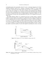
Figure 8.2: Boundary Conditions in Elasticity Problems
8.3 Boundary Value Problem Formulation
9 Hence, the boundary value formulation is suumarized by
∂T
ij
∂X
j
+ ρb
i
= ρ
∂
2
u
i
∂t
2
in Ω (8.4)
E

∗
=
1
2
(u∇
x
+ ∇
x
u) (8.5)
T = λI
E
+2µE in Ω (8.6)
u =
u in Γ
u
(8.7)
t =
t in Γ
t
(8.8)
and is illustrated by Fig. 8.3. This is now a well posed problem.
8.4 †Compact Forms
10 Solving a boundary value problem with 15 unknowns through 15 equations is a formidable task.
Hence, there are numerous methods to reformulate the problem in terms of fewer unknows.
8.4.1 Navier-Cauchy Equations
11 One such approach is to substitute the displacement-strain relation into Hooke’s law (resulting in
stresses in terms of the gradient of the displacement), and the resulting equation into the equation of
motion to obtain three second-order partial differential equations for the three displacement components
known as Navier’s Equation
(λ + µ)

∂
2
u
k
∂X
i
∂X
k
+ µ
∂
2
u
i
∂X
k
∂X
k
+ ρb
i
= ρ
∂
2
u
i
∂t
2
(8.9)
or
(λ + µ)∇(∇·u)+µ∇
2

u + ρb = ρ
∂
2
u
∂t
2
(8.10)
(8.11)
Victor Saouma Mechanics of Materials II
Draft
4 BOUNDARY VALUE PROBLEMS in ELASTICITY
Natural B.C.
t
i
:Γ
t
Stresses
T
ij
Equilibrium
∂T
ij
∂x
j
+ ρb
i
= ρ
dv
i
dt

Body Forces
b
i
Constitutive Rel.
T = λI
E
+2µE
Strain
E
ij
Kinematics
E
∗
=
1
2
(u∇
x
+ ∇
x
u)
Displacements
u
i
Essential B.C.
u
i
:Γ
u
✻

❄
❄
❄
❄
❄
✲ ✛
Figure 8.3: Fundamental Equations in Solid Mechanics
8.4.2 Beltrami-Mitchell Equations
12 Whereas Navier-Cauchy equation was expressed in terms of the gradient of the displacement, we can
follow a similar approach and write a single equation in term of the gradient of the tractions.
∇
2
T
ij
+
1
1+ν
T
pp,ij
= −
ν
1 − ν
δ
ij
∇·(ρb) − ρ(b
i,j
+ b
j,i
) (8.12)
or

T
ij,pp
+
1
1+ν
T
pp,ij
= −
ν
1 − ν
δ
ij
ρb
p,p
− ρ(b
i,j
+ b
j,i
) (8.13)
8.4.3 Airy Stress Function
Airy stress function, for plane strain problems will be separately covered in Sect. 9.2.
8.4.4 Ellipticity of Elasticity Problems
8.5 †Strain Energy and Extenal Work
13 For the isotropic Hooke’s law, we saw that there always exist a strain energy function W which is
positive-definite, homogeneous quadratic function of the strains such that, Eq. 18.29
T
ij
=
∂W
∂E

ij
(8.14)
hence it follows that
W =
1
2
T
ij
E
ij
(8.15)
Victor Saouma Mechanics of Materials II
Draft
8.6 †Uniqueness of the Elastostatic Stress and Strain Field 5
14 The external work done by a body in equilibrium under body forces b
i
and surface traction t
i
is
equal to

Ω
ρb
i
u
i
dΩ+

Γ
t

i
u
i
dΓ. Substituting t
i
= T
ij
n
j
and applying Gauss theorem, the second term
becomes

Γ
T
ij
n
j
u
i
dΓ=

Ω
(T
ij
u
i
)
,j
dΩ=


Ω
(T
ij,j
u
i
+ T
ij
u
i,j
)dΩ (8.16)
but T
ij
u
i,j
= T
ij
(E
ij
+Ω
ij
)=T
ij
E
ij
and from equilibrium T
ij,j
= −ρb
i
,thus


Ω
ρb
i
u
i
dΩ+

Γ
t
i
u
i
dΓ=

Ω
ρb
i
u
i
dΩ+

Ω
(T
ij
E
ij
− ρb
i
u
i

)dΩ (8.17)
or

Ω
ρb
i
u
i
dΩ+

Γ
t
i
u
i
dΓ

 
External Work
=2

Ω
T
ij
E
ij
2
dΩ

 

Internal Strain Energy
(8.18)
that is For an elastic system, the total strain energy is one half the work done by the external forces
acting through their displacements u
i
.
8.6 †Uniqueness of the Elastostatic Stress and Strain Field
15 Because the equations of linear elasticity are linear equations, the principles of superposition may be
used to obtain additional solutions from those established. Hence, given two sets of solution T
(1)
ij
, u
(1)
i
,
and T
(2)
ij
, u
(2)
i
, then T
ij
= T
(2)
ij
− T
(1)
ij
,andu

i
= u
(2)
i
− u
(1)
i
with b
i
= b
(2)
i
− b
(1)
i
= 0 must also be a
solution.
16 Hence for this “difference” solution, Eq. 8.18 would yield

Γ
t
i
u
i
dΓ=2

Ω
u
∗
dΩ but the left hand

side is zero because t
i
= t
(2)
i
− t
(1)
i
=0onΓ
u
,andu
i
= u
(2)
i
− u
(1)
i
=0onΓ
t
,thus

Ω
u
∗
dΩ=0.
17 But u
∗
is positive-definite and continuous, thus the integral can vanish if and only if u
∗

= 0 everywhere,
and this is only possible if E
ij
= 0 everywhere so that
E
(2)
ij
= E
(1)
ij
⇒ T
(2)
ij
= Tij
(1)
(8.19)
hence, there can not be two different stress and strain fields corresponding to the same externally imposed
body forces and boundary conditions
1
and satisfying the linearized elastostatic Eqs 8.1, 8.14 and 8.3.
8.7 Saint Venant’s Principle
18 This famous principle of Saint Venant was enunciated in 1855 and is of great importance in applied
elasticity where it is often invoked to justify certain “simplified” solutions to complex problem.
In elastostatics, if the boundary tractions on a part Γ
1
of the boundary Γ are replaced by a
statically equivalent traction distribution, the effects on the stress distribution in the body
are negligible at points whose distance from Γ
1
is large compared to the maximum distance

between points of Γ
1
.
19 For instance the analysis of the problem in Fig. 8.4 can be greatly simplified if the tractions on Γ
1
are replaced by a concentrated statically equivalent force.
1
This theorem is attributed to Kirchoff (1858).
Victor Saouma Mechanics of Materials II
Draft
6 BOUNDARY VALUE PROBLEMS in ELASTICITY
F=tdx
t
dx
Figure 8.4: St-Venant’s Principle
8.8 Cylindrical Coordinates
20 So far all equations have been written in either vector, indicial, or engineering notation. The last two
were so far restricted to an othonormal cartesian coordinate system.
21 We now rewrite some of the fundamental relations in cylindrical coordinate system, Fig. 8.5, as
this would enable us to analytically solve some simple problems of great practical usefulness (torsion,
pressurized cylinders, ). This is most often achieved by reducing the dimensionality of the problem
from3to2orevento1.
z
θ
r
Figure 8.5: Cylindrical Coordinates
8.8.1 Strains
22 With reference to Fig. 8.6, we consider the displacement of point P to P
∗
. the displacements can be

expressed in cartesian coordinates as u
x
,u
y
, or in polar coordinates as u
r
,u
θ
. Hence,
u
x
= u
r
cos θ −u
θ
sin θ (8.20-a)
u
y
= u
r
sin θ + u
θ
cos θ (8.20-b)
Victor Saouma Mechanics of Materials II
Draft
8.8 Cylindrical Coordinates 7
u
u
u
*

x
y
r
θ
u
θ
r
x
y
P
P
θ
θ
Figure 8.6: Polar Strains
substituting into the strain definition for ε
xx
(for small displacements) we obtain
ε
xx
=
∂u
x
∂x
=
∂u
x
∂θ
∂θ
∂x
+

∂u
x
∂r
∂r
∂x
(8.21-a)
∂u
x
∂θ
=
∂u
r
∂θ
cos θ −u
r
sin θ −
∂u
θ
∂θ
sin θ −u
θ
cos θ (8.21-b)
∂u
x
∂r
=
∂u
r
∂r
cos θ −

∂u
θ
∂r
sin θ (8.21-c)
∂θ
∂x
= −
sin θ
r
(8.21-d)
∂r
∂x
=cosθ (8.21-e)
ε
xx
=

−
∂u
r
∂θ
cos θ + u
r
sin θ +
∂u
θ
∂θ
sin θ + u
θ
cos θ


sin θ
r
+

∂u
r
∂r
cos θ −
∂u
θ
∂r
sin θ

cos θ (8.21-f)
Noting that as θ → 0, ε
xx
→ ε
rr
,sinθ → 0, and cos θ → 1, we obtain
ε
rr
= ε
xx
|
θ→0
=
∂u
r
∂r

(8.22)
23 Similarly, if θ → π/2, ε
xx
→ ε
θθ
,sinθ → 1, and cos θ → 0. Hence,
ε
θθ
= ε
xx
|
θ→π/2
=
1
r
∂u
θ
∂θ
+
u
r
r
(8.23)
finally, we may express ε
xy
as a function of u
r
,u
θ
and θ and noting that ε

xy
→ ε
rθ
as θ → 0, we obtain
ε
rθ
=
1
2

ε
xy
|
θ→0
=
∂u
θ
∂r
−
u
θ
r
+
1
r
∂u
r
∂θ

(8.24)

24 In summary, and with the addition of the z components (not explicitely derived), we obtain
Victor Saouma Mechanics of Materials II
Draft
8 BOUNDARY VALUE PROBLEMS in ELASTICITY
ε
rr
=
∂u
r
∂r
(8.25)
ε
θθ
=
1
r
∂u
θ
∂θ
+
u
r
r
(8.26)
ε
zz
=
∂u
z
∂z

(8.27)
ε
rθ
=
1
2

1
r
∂u
r
∂θ
+
∂u
θ
∂r
−
u
θ
r

(8.28)
ε
θz
=
1
2

∂u
θ

∂z
+
1
r
∂u
z
∂θ

(8.29)
ε
rz
=
1
2

∂u
z
∂r
+
∂u
r
∂z

(8.30)
8.8.2 Equilibrium
25 Whereas the equilibrium equation as given In Eq. 6.17 was obtained from the linear momentum
principle (without any reference to the notion of equilibrium of forces), its derivation (as mentioned)
could have been obtained by equilibrium of forces considerations. This is the approach which we will
follow for the polar coordinate system with respect to Fig. 8.7.
δ

θ
θ
d
θ
d
d
r
d
r
θθ
rr
δ
δ
θr
+
r
r+dr
θ
θd
r
f
f
r
θ
δ
δ
θ
θr
+
+

δ
δ
rr
r
θr
T
r
r
r θ
θr
T
T
T
T
T
T
T
T
+
δ
θθ
θθ
T
T
Figure 8.7: Stresses in Polar Coordinates
26 Summation of forces parallel to the radial direction through the center of the element with unit
thickness in the z direction yields:

T
rr

+
∂T
rr
∂r
dr

(r + dr)dθ −T
rr
(rdθ)
−

T
θθ
+
∂T
θθ
∂θ
+ T
θθ

dr sin
dθ
2
+

T
θr
+
∂T
θr

∂θ
dθ −T
θr

dr cos
dθ
2
+ f
r
rdrdθ =0
(8.31)
we approximate sin(dθ/2) by dθ/2 and cos(dθ/2) by unity, divide through by rdrdθ,
1
r
T
rr
+
∂T
rr
∂r

1+
dr
r

−
T
θθ
r
−

∂T
θθ
∂θ
dθ
dr
+
1
r
∂T
θr
∂θ
+ f
r
= 0 (8.32)
27 Similarly we can take the summation of forces in the θ direction. In both cases if we were to drop the
dr/r and dθ/r in the limit, we obtain
Victor Saouma Mechanics of Materials II
Draft
8.8 Cylindrical Coordinates 9
∂T
rr
∂r
+
1
r
∂T
θr
∂θ
+
1

r
(T
rr
− T
θθ
)+f
r
= 0 (8.33)
∂T
rθ
∂r
+
1
r
∂T
θθ
∂θ
+
1
r
(T
rθ
− T
θr
)+f
θ
= 0 (8.34)
28 It is often necessary to express cartesian stresses in terms of polar stresses and vice versa. This can
be done through the following relationships


T
xx
T
xy
T
xy
T
yy

=

cos θ −sin θ
sin θ cos θ

T
rr
T
rθ
T
rθ
T
θθ

cos θ −sin θ
sin θ cos θ

T
(8.35)
yielding
T

xx
= T
rr
cos
2
θ + T
θθ
sin
2
θ −T
rθ
sin 2θ (8.36-a)
T
yy
= T
rr
sin
2
θ + T
θθ
cos
2
θ + T
rθ
sin 2θ (8.36-b)
T
xy
=(T
rr
− T

θθ
)sinθ cos θ + T
rθ
(cos
2
θ −sin
2
θ) (8.36-c)
(recalling that sin
2
θ =1/2sin2θ, and cos
2
θ =1/2(1 + cos 2θ)).
8.8.3 Stress-Strain Relations
29 In orthogonal curvilinear coordinates, the physical components of a tensor at a point are merely the
Cartesian components in a local coordinate system at the point with its axes tangent to the coordinate
curves. Hence,
T
rr
= λe +2µε
rr
(8.37)
T
θθ
= λe +2µε
θθ
(8.38)
T
rθ
=2µε

rθ
(8.39)
T
zz
= ν(T
rr
+ T
θθ
) (8.40)
with e = ε
rr
+ ε
θθ
. alternatively,
E
rr
=
1
E

(1 − ν
2
)T
rr
− ν(1 + ν)T
θθ

(8.41)
E
θθ

=
1
E

(1 − ν
2
)T
θθ
− ν(1 + ν)T
rr

(8.42)
E
rθ
=
1+ν
E
T
rθ
(8.43)
E
rz
= E
θz
= E
zz
= 0 (8.44)
8.8.3.1 Plane Strain
30 For Plane strain problems, from Eq. 7.52:








σ
rr
σ
θθ
σ
zz
τ
rθ







=
E
(1 + ν)(1 − 2ν)




(1 − ν) ν 0
ν (1 − ν)0

νν0
00
1−2ν
2







ε
rr
ε
θθ
γ
rθ



(8.45)
and ε
zz
= γ
rz
= γ
θz
= τ
rz
= τ

θz
=0.
31 Inverting,



ε
rr
ε
θθ
γ
rθ



=
1
E




1 − ν
2
−ν(1 + ν)0
−ν(1 + ν)1− ν
2
0
νν0
0 0 2(1 + ν












σ
rr
σ
θθ
σ
zz
τ
rθ







(8.46)
Victor Saouma Mechanics of Materials II
Draft
10 BOUNDARY VALUE PROBLEMS in ELASTICITY

8.8.3.2 Plane Stress
32 For plane stress problems, from Eq. 7.55-a



σ
rr
σ
θθ
τ
rθ



=
E
1 − ν
2


1 ν 0
ν 10
00
1−ν
2






ε
rr
ε
θθ
γ
rθ



(8.47-a)
ε
zz
= −
1
1 − ν
ν(ε
rr
+ ε
θθ
) (8.47-b)
and τ
rz
= τ
θz
= σ
zz
= γ
rz
= γ
θz

=0
33 Inverting



ε
rr
ε
θθ
γ
rθ



=
1
E


1 −ν 0
−ν 10
0 0 2(1 + ν)





σ
rr
σ

θθ
τ
rθ



(8.48-a)
Victor Saouma Mechanics of Materials II
Draft
Chapter 9
SOME ELASTICITY PROBLEMS
1 Practical solutions of two-dimensional boundary-value problem in simply connected regions can be
accomplished by numerous techniques. Those include: a) Finite-difference approximation of the dif-
ferential equation, b) Complex function method of Muskhelisvili (most useful in problems with stress
concentration), c) Variational methods, d) Semi-inverse methods, and e) Airy stress functions.
2 Only the last two methods will be discussed in this chapter.
9.1 Semi-Inverse Method
3 Often a solution to an elasticity problem may be obtained without seeking simulateneous solutions to
the equations of motion, Hooke’s Law and boundary conditions. One may attempt to seek solutions
by making certain assumptions or guesses about the components of strain stress or displacement while
leaving enough freedom in these assumptions so that the equations of elasticity be satisfied.
4 If the assumptions allow us to satisfy the elasticity equations, then by the uniqueness theorem, we
have succeeded in obtaining the solution to the problem.
5 This method was employed by Saint-Venant in his treatment of the torsion problem, hence it is often
referred to as the Saint-Venant semi-inverse method.
9.1.1 Example: Torsion of a Circular Cylinder
6 Let us consider the elastic deformation of a cylindrical bar with circular cross section of radius a and
length L twisted by equal and opposite end moments M
1
, Fig. 9.1.

7 From symmetry, it is reasonable to assume that the motion of each cross-sectional plane is a rigid body
rotation about the x
1
axis. Hence, for a small rotation angle θ, the displacement field will be given by:
u =(θe
1
)×r =(θe
1
)×(x
1
e
1
+ x
2
e
2
+ x
3
e
3
)=θ(x
2
e
3
− x
3
e
2
) (9.1)
or

u
1
=0; u
2
= −θx
3
; u
3
= θx
2
(9.2)
where θ = θ(x
1
).
8 The corresponding strains are given by
E
11
= E
22
= E
33
= 0 (9.3-a)
E
12
= −
1
2
x
3
∂θ

∂x
1
(9.3-b)
Draft
2 SOME ELASTICITY PROBLEMS
X
X
XL
M
M
1
2
3
T
T
aθ
n
n
Figure 9.1: Torsion of a Circular Bar
E
13
=
1
2
x
2
∂θ
∂x
1
(9.3-c)

9 The non zero stress components are obtained from Hooke’s law
T
12
= −µx
3
∂θ
∂x
1
(9.4-a)
T
13
= µx
2
∂θ
∂x
1
(9.4-b)
10 We need to check that this state of stress satisfies equilibrium ∂T
ij
/∂x
j
= 0. The first one j =1is
identically satisfied, whereas the other two yield
−µx
3
d
2
θ
dx
2

1
= 0 (9.5-a)
µx
2
d
2
θ
dx
2
1
= 0 (9.5-b)
thus,
dθ
dx
1
≡ θ

= constant (9.6)
Physically, this means that equilibrium is only satisfied if the increment in angular rotation (twist per
unit length) is a constant.
11 We next determine the corresponding surface tractions. On the lateral surface we have a unit normal
vector n =
1
a
(x
2
e
2
+ x
3

e
3
), therefore the surface traction on the lateral surface is given by
{t} =[T]{n} =
1
a


0 T
12
T
13
T
21
00
T
31
00





0
x
2
x
3




=
1
a



x
2
T
12
0
0



(9.7)
12 Substituting,
t =
µ
a
(−x
2
x
3
θ

+ x
2
x

3
θ

)e
1
= 0 (9.8)
which is in agreement with the fact that the bar is twisted by end moments only, the lateral surface is
traction free.
Victor Saouma Mechanics of Materials II
Draft
9.2 Airy Stress Functions; Plane Strain 3
13 On the face x
1
= L, we have a unit normal n = e
1
and a surface traction
t = Te
1
= T
21
e
2
+ T
31
e
3
(9.9)
this distribution of surface traction on the end face gives rise to the following resultants
R
1

=

T
11
dA = 0 (9.10-a)
R
2
=

T
21
dA = µθ


x
3
dA = 0 (9.10-b)
R
3
=

T
31
dA = µθ


x
2
dA = 0 (9.10-c)
M

1
=

(x
2
T
31
− x
3
T
21
)dA = µθ


(x
2
2
+ x
2
3
)dA = µθ

J (9.10-d)
M
2
= M
3
= 0 (9.10-e)
We note that


(x
2
2
+ x
3
3
)
2
dA is the polar moment of inertia of the cross section and is equal to
J = πa
4
/2, and we also note that

x
2
dA =

x
3
dA = 0 because the area is symmetric with respect to
the axes.
14 From the last equation we note that
θ

=
M
µJ
(9.11)
which implies that the shear modulus µ can be determined froma simple torsion experiment.
15 Finally, in terms of the twisting couple M, the stress tensor becomes

[T]=


0 −
Mx
3
J
Mx
2
J
−
Mx
3
J
00
Mx
2
J
00


(9.12)
9.2 Airy Stress Functions; Plane Strain
16 If the deformation of a cylindrical body is such that there is no axial components of the displacement
and that the other components do not depend on the axial coordinate, then the body is said to be in a
state of plane strain. If e
3
is the direction corresponding to the cylindrical axis, then we have
u
1

= u
1
(x
1
,x
2
),u
2
= u
2
(x
1
,x
2
),u
3
= 0 (9.13)
and the strain components corresponding to those displacements are
E
11
=
∂u
1
∂x
1
(9.14-a)
E
22
=
∂u

2
∂x
2
(9.14-b)
E
12
=
1
2

∂u
1
∂x
2
+
∂u
2
∂x
1

(9.14-c)
E
13
= E
23
= E
33
= 0 (9.14-d)
and the non-zero stress components are T
11

,T
12
,T
22
,T
33
where
T
33
= ν(T
11
+ T
22
) (9.15)
Victor Saouma Mechanics of Materials II
Draft
4 SOME ELASTICITY PROBLEMS
17 Considering a static stress field with no body forces, the equilibrium equations reduce to:
∂T
11
∂x
1
+
∂T
12
∂x
2
= 0 (9.16-a)
∂T
12

∂x
1
+
∂T
22
∂x
2
= 0 (9.16-b)
∂T
33
∂x
1
= 0 (9.16-c)
we note that since T
33
= T
33
(x
1
,x
2
), the last equation is always satisfied.
18 Hence, it can be easily verified that for any arbitrary scalar variable Φ, if we compute the stress
components from
T
11
=
∂
2
Φ

∂x
2
2
(9.17)
T
22
=
∂
2
Φ
∂x
2
1
(9.18)
T
12
= −
∂
2
Φ
∂x
1
∂x
2
(9.19)
then the first two equations of equilibrium are automatically satisfied. This function Φ is called Airy
stress function.
19 However, if stress components determined this way are statically admissible (i.e. they satisfy
equilibrium), they are not necessarily kinematically admissible (i.e. satisfy compatibility equations).
20 To ensure compatibility of the strain components, we express the strains components in terms of Φ

from Hooke’s law, Eq. 7.36 and Eq. 9.15.
E
11
=
1
E

(1 − ν
2
)T
11
− ν(1 + ν)T
22

=
1
E

(1 − ν
2
)
∂
2
Φ
∂x
2
2
− ν(1 + ν)
∂
2

Φ
∂x
2
1

(9.20-a)
E
22
=
1
E

(1 − ν
2
)T
22
− ν(1 + ν)T
11

=
1
E

(1 − ν
2
)
∂
2
Φ
∂x

2
1
− ν(1 + ν)
∂
2
Φ
∂x
2
2

(9.20-b)
E
12
=
1
E
(1 + ν)T
12
= −
1
E
(1 + ν)
∂
2
Φ
∂x
1
∂x
2
(9.20-c)

For plane strain problems, the only compatibility equation, 4.140, that is not automatically satisfied is
∂
2
E
11
∂x
2
2
+
∂
2
E
22
∂x
2
1
=2
∂
2
E
12
∂x
1
∂x
2
(9.21)
substituting,
(1 − ν)

∂

4
Φ
∂x
4
1
+2
∂
4
Φ
∂x
2
1
∂x
2
2
+
∂
4
Φ
∂x
4
1

= 0 (9.22)
or
∂
4
Φ
∂x
4

1
+2
∂
4
Φ
∂x
2
1
∂x
2
2
+
∂
4
Φ
∂x
4
2
=0 or ∇
4
Φ=0
(9.23)
Hence, any function which satisfies the preceding equation will satisfy both equilibrium, kinematic,
stress-strain (albeit plane strain) and is thus an acceptable elasticity solution.
21 †We can also obtain from the Hooke’s law, the compatibility equation 9.21, and the equilibrium
equations the following

∂
2
∂x

2
1
+
∂
2
∂x
2
2

(T
11
+ T
22
)=0 or ∇
2
(T
11
+ T
22
)=0
(9.24)
Victor Saouma Mechanics of Materials II
Draft
9.2 Airy Stress Functions; Plane Strain 5
22 †Any polynomial of degree three or less in x and y satisfies the biharmonic equation (Eq. 9.23). A
systematic way of selecting coefficients begins with
Φ=
∞

m=0

∞

n=0
C
mn
x
m
y
n
(9.25)
23 †The stresses will be given by
T
xx
=
∞

m=0
∞

n=2
n(n − 1)C
mn
x
m
y
n−2
(9.26-a)
T
yy
=

∞

m=2
∞

n=0
m(m − 1)C
mn
x
m−1
y
n
(9.26-b)
T
xy
= −
∞

m=1
∞

n=1
mnC
mn
x
m−1
y
n−1
(9.26-c)
24 †Substituting into Eq. 9.23 and regrouping we obtain

∞

m=2
∞

n=2
[(m+2)(m+1)m(m−1)C
m+2,n−2
+2m(m−1)n(n−1)C
mn
+(n+2)(n+1)n(n−1)C
m−2,n+2
]x
m−2
y
n−2
=0
(9.27)
but since the equation must be identically satisfied for all x and y, the term in bracket must be equal to
zero.
(m+2)(m+1)m(m−1)C
m+2,n−2
+2m(m−1)n(n−1)C
mn
+(n+2)(n+1)n(n−1)C
m−2,n+2
= 0 (9.28)
Hence, the recursion relation establishes relationships among groups of three alternate coefficients which
can be selected from












00C
02
C
03
C
04
C
05
C
06
···
0 C
11
C
12
C
13
C
14
C

15
···
C
20
C
21
C
22
C
23
C
24
···
C
30
C
31
C
32
C
33
···
C
40
C
41
C
42
···
C50 C

51
···
C
60
···











(9.29)
For example if we consider m = n = 2, then
(4)(3)(2)(1)C
40
+ (2)(2)(1)(2)(1)C
22
+ (4)(3)(2)(1)C
04
= 0 (9.30)
or 3C
40
+ C
22
+3C

04
=0
9.2.1 Example: Cantilever Beam
25 We consider the homogeneous fourth-degree polynomial
Φ
4
= C
40
x
4
+ C
31
x
3
y + C
22
x
2
y
2
+ C
13
xy
3
+ C
04
y
4
(9.31)
with 3C

40
+ C
22
+3C
04
=0,
26 The stresses are obtained from Eq. 9.26-a-9.26-c
T
xx
=2C
22
x
2
+6C
13
xy +12C
04
y
2
(9.32-a)
T
yy
=12C
40
x
2
+6C
31
xy +2C
22

y
2
(9.32-b)
T
xy
= −3C
31
x
2
− 4C
22
xy −3C
13
y
2
(9.32-c)
Victor Saouma Mechanics of Materials II
Draft
6 SOME ELASTICITY PROBLEMS
These can be used for the end-loaded cantilever beam with width b along the z axis, depth 2a and
length L.
27 If all coefficients except C
13
are taken to be zero, then
T
xx
=6C
13
xy (9.33-a)
T

yy
= 0 (9.33-b)
T
xy
= −3C
13
y
2
(9.33-c)
28 This will give a parabolic shear traction on the loaded end (correct), but also a uniform shear traction
T
xy
= −3C
13
a
2
on top and bottom. These can be removed by superposing uniform shear stress T
xy
=
+3C
13
a
2
corresponding to Φ
2
= −3C
13
a
2
  

C
11
xy.Thus
T
xy
=3C
13
(a
2
− y
2
) (9.34)
note that C
20
= C
02
=0,andC
11
= −3C
13
a
2
.
29 The constant C
13
is determined by requiring that
P = b

a
−a

−T
xy
dy = −3bC
13

a
−a
(a
2
− y
2
)dy (9.35)
hence
C
13
= −
P
4a
3
b
(9.36)
and the solution is
Φ=
3P
4ab
xy −
P
4a
3
b

xy
3
(9.37-a)
T
xx
= −
3P
2a
3
b
xy (9.37-b)
T
xy
= −
3P
4a
3
b
(a
2
− y
2
) (9.37-c)
T
yy
= 0 (9.37-d)
30 We observe that the second moment of area for the rectangular cross section is I = b(2a)
3
/12 = 2a
3

b/3,
hence this solution agrees with the elementary beam theory solution
Φ=C
11
xy + C
13
xy
3
=
3P
4ab
xy −
P
4a
3
b
xy
3
(9.38-a)
T
xx
= −
P
I
xy = −M
y
I
= −
M
S

(9.38-b)
T
xy
= −
P
2I
(a
2
− y
2
) (9.38-c)
T
yy
= 0 (9.38-d)
9.2.2 Polar Coordinates
9.2.2.1 Plane Strain Formulation
31 In polar coordinates, the strain components in plane strain are, Eq. 8.46
E
rr
=
1
E

(1 − ν
2
)T
rr
− ν(1 + ν)T
θθ


(9.39-a)
Victor Saouma Mechanics of Materials II
Draft
9.2 Airy Stress Functions; Plane Strain 7
E
θθ
=
1
E

(1 − ν
2
)T
θθ
− ν(1 + ν)T
rr

(9.39-b)
E
rθ
=
1+ν
E
T
rθ
(9.39-c)
E
rz
= E
θz

= E
zz
= 0 (9.39-d)
and the equations of equilibrium are
1
r
∂T
rr
∂r
+
1
r
∂T
θr
∂θ
−
T
θθ
r
= 0 (9.40-a)
1
r
2
∂T
rθ
∂r
+
1
r
∂T

θθ
∂θ
= 0 (9.40-b)
32 Again, it can be easily verified that the equations of equilibrium are identically satisfied if
T
rr
=
1
r
∂Φ
∂r
+
1
r
2
∂
2
Φ
∂θ
2
(9.41)
T
θθ
=
∂
2
Φ
∂r
2
(9.42)

T
rθ
= −
∂
∂r

1
r
∂Φ
∂θ

(9.43)
33 In order to satisfy the compatibility conditions, the cartesian stress components must also satisfy Eq.
9.24. To derive the equivalent expression in cylindrical coordinates, we note that T
11
+ T
22
is the first
scalar invariant of the stress tensor, therefore
T
11
+ T
22
= T
rr
+ T
θθ
=
1
r

∂Φ
∂r
+
1
r
2
∂
2
Φ
∂θ
2
+
∂
2
Φ
∂r
2
(9.44)
34 We also note that in cylindrical coordinates, the Laplacian operator takes the following form
∇
2
=
∂
2
∂r
2
+
1
r
∂

∂r
+
1
r
2
∂
2
∂θ
2
(9.45)
35 Thus, the function Φ must satisfy the biharmonic equation

∂
2
∂r
2
+
1
r
∂
∂r
+
1
r
2
∂
2
∂θ
2


∂
2
∂r
2
+
1
r
∂
∂r
+
1
r
2
∂
2
∂θ
2

=0 or ∇
4
=0
(9.46)
9.2.2.2 Axially Symmetric Case
36 If Φ is a function of r only, we have
T
rr
=
1
r
dΦ

dr
; T
θθ
=
d
2
Φ
dr
2
; T
rθ
= 0 (9.47)
and
d
4
Φ
dr
4
+
2
r
d
3
Φ
dr
3
−
1
r
2

d
2
Φ
dr
2
+
1
r
3
dΦ
dr
= 0 (9.48)
37 The general solution to this problem; using Mathematica:
DSolve[phi’’’’[r]+2 phi’’’[r]/r-phi’’[r]/r^2+phi’[r]/r^3==0,phi[r],r]
Victor Saouma Mechanics of Materials II
Draft
8 SOME ELASTICITY PROBLEMS
Φ=A ln r + Br
2
ln r + Cr
2
+ D (9.49)
38 The corresponding stress field is
T
rr
=
A
r
2
+ B(1 + 2 ln r)+2C (9.50)

T
θθ
= −
A
r
2
+ B(3 + 2 ln r)+2C (9.51)
T
rθ
= 0 (9.52)
and the strain components are (from Sect. 8.8.1)
E
rr
=
∂u
r
∂r
=
1
E

(1 + ν)A
r
2
+(1− 3ν − 4ν
2
)B + 2(1 − ν − 2ν
2
)B ln r + 2(1 − ν −2ν
2

)C

(9.53)
E
θθ
=
1
r
∂u
θ
∂θ
+
u
r
r
=
1
E

−
(1 + ν)A
r
2
+(3− ν − 4ν
2
)B + 2(1 − ν − 2ν
2
)B ln r + 2(1 − ν −2ν
2
)C


(9.54)
E
rθ
=0 (9.55)
39 Finally, the displacement components can be obtained by integrating the above equations
u
r
=
1
E

−
(1 + ν)A
r
− (1 + ν)Br + 2(1 −ν − 2ν
2
)r ln rB + 2(1 −ν −2ν
2
)rC

(9.56)
u
θ
=
4rθB
E
(1 − ν
2
) (9.57)

9.2.2.3 Example: Thick-Walled Cylinder
40 If we consider a circular cylinder with internal and external radii a and b respectively, subjected to
internal and external pressures p
i
and p
o
respectively, Fig. 9.2, then the boundary conditions for the
plane strain problem are
T
rr
= −p
i
at r = a (9.58-a)
T
rr
= −p
o
at r = b (9.58-b)
Saint Venant
a
b
p
i
o
p
Figure 9.2: Pressurized Thick Tube
41 These Boundary conditions can be easily shown to be satisfied by the following stress field
T
rr
=

A
r
2
+2C (9.59-a)
T
θθ
= −
A
r
2
+2C (9.59-b)
T
rθ
= 0 (9.59-c)
Victor Saouma Mechanics of Materials II
Draft
9.2 Airy Stress Functions; Plane Strain 9
These equations are taken from Eq. 9.50, 9.51 and 9.52 with B = 0 and therefore represent a possible
state of stress for the plane strain problem.
42 We note that if we take B = 0, then u
θ
=
4rθB
E
(1 −ν
2
) and this is not acceptable because if we were
to start at θ = 0 and trace a curve around the origin and return to the same point, than θ =2π and the
displacement would then be different.
43 Applying the boundary condition we find that

T
rr
= −p
i
(b
2
/r
2
) − 1
(b
2
/a
2
) − 1
− p
0
1 − (a
2
/r
2
)
1 − (a
2
/b
2
)
(9.60)
T
θθ
= p

i
(b
2
/r
2
)+1
(b
2
/a
2
) − 1
− p
0
1+(a
2
/r
2
)
1 − (a
2
/b
2
)
(9.61)
T
rθ
= 0 (9.62)
44 We note that if only the internal pressure p
i
is acting, then T

rr
is always a compressive stress, and
T
θθ
is always positive.
45 If the cylinder is thick, then the strains are given by Eq. 9.53, 9.54 and 9.55. For a very thin cylinder
in the axial direction, then the strains will be given by
E
rr
=
du
dr
=
1
E
(T
rr
− νT
θθ
) (9.63-a)
E
θθ
=
u
r
=
1
E
(T
θθ

− νT
rr
) (9.63-b)
E
zz
=
dw
dz
=
ν
E
(T
rr
+ T
θθ
) (9.63-c)
E
rθ
=
(1 + ν)
E
T
rθ
(9.63-d)
46 It should be noted that applying Saint-Venant’s principle the above solution is only valid away from
the ends of the cylinder.
9.2.2.4 Example: Hollow Sphere
47 We consider next a hollow sphere with internal and xternal radii a
i
and a

o
respectively, and subjected
to internal and external pressures of p
i
and p
o
, Fig. 9.3.
a
o
i
p
o
p
a
i
Figure 9.3: Pressurized Hollow Sphere
48 With respect to the spherical ccordinates (r,θ,φ), it is clear due to the spherical symmetry of the
geometry and the loading that each particle of the elastic sphere will expereince only a radial displacement
Victor Saouma Mechanics of Materials II
Draft
10 SOME ELASTICITY PROBLEMS
rr
r
θ
b
rr
σ
I
II
b

θ
θ
σ
τ
a
a
a
τ
r
θ
σ
o
θ
b
x
σ
rr
y
σ
o
Figure 9.4: Circular Hole in an Infinite Plate
whose magnitude depends on r only, that is
u
r
= u
r
(r),u
θ
= u
φ

= 0 (9.64)
9.3 Circular Hole, (Kirsch, 1898)
49 Analysing the infinite plate under uniform tension with a circular hole of diameter a, and subjected
to a uniform stress σ
0
, Fig. 9.4.
50 The peculiarity of this problem is that the far-field boundary conditions are better expressed in
cartesian coordinates, whereas the ones around the hole should be written in polar coordinate system.
51 We will solve this problem by replacing the plate with a thick tube subjected to two different set of
loads. The first one is a thick cylinder subjected to uniform radial pressure (solution of which is well
known from Strength of Materials), the second one is a thick cylinder subjected to both radial and shear
stresses which must be compatible with the traction applied on the rectangular plate.
52 First we select a stress function which satisfies the biharmonic Equation (Eq. ??), and the far-field
boundary conditions. From St Venant principle, away from the hole, the boundary conditions are given
by:
σ
xx
= σ
0
; σ
yy
= τ
xy
= 0 (9.65)
53 Recalling (Eq. 9.19) that σ
xx
=
∂
2
Φ

∂y
2
, this would would suggest a stress function Φ of the form
Φ=σ
0
y
2
. Alternatively, the presence of the circular hole would suggest a polar representation of Φ.
Thus, substituting y = r sin θ would result in Φ = σ
0
r
2
sin
2
θ.
54 Since sin
2
θ =
1
2
(1 − cos 2θ), we could simplify the stress function into
Φ=f(r)cos2θ (9.66)
55 Substituting this function into the biharmonic equation (Eq. ??) yields

∂
2
∂r
2
+
1

r
∂
∂r
+
1
r
2
∂
2
∂θ
2

∂
2
Φ
∂r
2
+
1
r
∂Φ
∂r
+
1
r
2
∂
2
Φ
∂θ

2

= 0 (9.67-a)

d
2
dr
2
+
1
r
d
dr
−
4
r
2

d
2
f
dr
2
+
1
r
df
dr
−
4f

r
2

= 0 (9.67-b)
(note that the cos 2θ term is dropped)
56 The general solution of this ordinary linear fourth order differential equation is
f(r)=Ar
2
+ Br
4
+ C
1
r
2
+ D (9.68)
Victor Saouma Mechanics of Materials II
Draft
9.3 Circular Hole, (Kirsch, 1898) 11
thus the stress function becomes
Φ=

Ar
2
+ Br
4
+ C
1
r
2
+ D


cos 2θ (9.69)
57 Next, we must determine the constants A, B, C,andD. Using Eq. ??, the stresses are given by
σ
rr
=
1
r
∂Φ
∂r
+
1
r
2
∂
2
Φ
∂θ
2
= −

2A +
6C
r
4
+
4D
r
2


cos 2θ
σ
θθ
=
∂
2
Φ
∂r
2
=

2A +12Br
2
+
6C
r
4

cos 2θ
τ
rθ
= −
∂
∂r

1
r
∂Φ
∂θ


=

2A +6Br
2
−
6C
r
4
−
2D
r
2

sin 2θ
(9.70)
58 Next we seek to solve for the four constants of integration by applying the boundary conditions. We
will identify two sets of boundary conditions:
1. Outer boundaries: around an infinitely large circle of radius b inside a plate subjected to uniform
stress σ
0
, the stresses in polar coordinates are obtained from Strength of Materials

σ
rr
σ
rθ
σ
rθ
σ
θθ


=

cos θ −sin θ
sin θ cos θ

σ
0
0
00

cos θ −sin θ
sin θ cos θ

T
(9.71)
yielding (recalling that sin
2
θ =1/2sin2θ, and cos
2
θ =1/2(1 + cos 2θ)).
(σ
rr
)
r=b
= σ
0
cos
2
θ =

1
2
σ
0
(1 + cos 2θ) (9.72-a)
(σ
rθ
)
r=b
=
1
2
σ
0
sin 2θ (9.72-b)
(σ
θθ
)
r=b
=
σ
0
2
(1 − cos 2θ) (9.72-c)
For reasons which will become apparent later, it is more convenient to decompose the state of
stress given by Eq. 9.72-a and 9.72-b, into state I and II:
(σ
rr
)
I

r=b
=
1
2
σ
0
(9.73-a)
(σ
rθ
)
I
r=b
= 0 (9.73-b)
(σ
rr
)
II
r=b
=
1
2
σ
0
cos 2θ
✛
(9.73-c)
(σ
rθ
)
II

r=b
=
1
2
σ
0
sin 2θ
✛
(9.73-d)
Where state I corresponds to a thick cylinder with external pressure applied on r = b and of
magnitude σ
0
/2. Hence, only the last two equations will provide us with boundary conditions.
2. Around the hole: the stresses should be equal to zero:
(σ
rr
)
r=a
=0
✛
(9.74-a)
(σ
rθ
)
r=a
=0
✛
(9.74-b)
59 Upon substitution in Eq. 9.70 the four boundary conditions (Eq. 9.73-c, 9.73-d, 9.74-a, and 9.74-b)
become

−

2A +
6C
b
4
+
4D
b
2

=
1
2
σ
0
(9.75-a)

2A +6Bb
2
−
6C
b
4
−
2D
b
2

=

1
2
σ
0
(9.75-b)
−

2A +
6C
a
4
+
4D
a
2

= 0 (9.75-c)

2A +6Ba
2
−
6C
a
4
−
2D
a
2

= 0 (9.75-d)

Victor Saouma Mechanics of Materials II
Draft
12 SOME ELASTICITY PROBLEMS
60 Solving for the four unknowns, and taking
a
b
= 0 (i.e. an infinite plate), we obtain:
A = −
σ
0
4
; B =0; C = −
a
4
4
σ
0
; D =
a
2
2
σ
0
(9.76)
61 To this solution, we must superimpose the one of a thick cylinder subjected to a uniform radial traction
σ
0
/2 on the outer surface, and with b much greater than a (Eq. 9.73-a and 9.73-b. These stresses are
obtained from Strength of Materials yielding for this problem (carefull about the sign)
σ

rr
=
σ
0
2

1 −
a
2
r
2

(9.77-a)
σ
θθ
=
σ
0
2

1+
a
2
r
2

(9.77-b)
62 Thus, substituting Eq. 9.75-a- into Eq. 9.70, we obtain
σ
rr

=
σ
0
2

1 −
a
2
r
2

+

1+3
a
4
r
4
−
4a
2
r
2

1
2
σ
0
cos 2θ (9.78-a)
σ

θθ
=
σ
0
2

1+
a
2
r
2

−

1+
3a
4
r
4

1
2
σ
0
cos 2θ (9.78-b)
σ
rθ
= −

1 −

3a
4
r
4
+
2a
2
r
2

1
2
σ
0
sin 2θ (9.78-c)
63 We observe that as r →∞, both σ
rr
and σ
rθ
are equal to the values given in Eq. 9.72-a and 9.72-b
respectively.
64 Alternatively, at the edge of the hole when r = a we obtain
σ
rr
= 0 (9.79)
σ
rθ
= 0 (9.80)
σ
θθ

|
r=a
= σ
0
(1 − 2cos2θ) (9.81)
which for θ =
π
2
and
3π
2
gives a stress concentration factor (SCF) of 3. For θ =0andθ = π, σ
θθ
= −σ
0
.
Victor Saouma Mechanics of Materials II