Mobile Robots Perception & Navigation Part 8 pdf
Bạn đang xem bản rút gọn của tài liệu. Xem và tải ngay bản đầy đủ của tài liệu tại đây (699.51 KB, 40 trang )
Global Navigation of Assistant Robots using Partially Observable Markov Decision Processes 271
4.3. Action and observation uncertainties
Besides the topology of the environment, it’s necessary to define some action and
observation uncertainties to generate the final POMDP model (transition and observation
matrixes). A first way of defining these uncertainties is by introducing some experimental
“hand-made” rules (this method is used in (Koenig & Simmons, 1998) and (Zanichelli,
1999)). For example, if a “Follow” action (a
F
) is commanded, the expected probability of
making a state transition (F) is 70%, while there is a 10% probability of remaining in the
same state (N=no action), a 10% probability of making two successive state transitions (FF),
and a 10% probability of making three state transitions (FFF). Experience with this method
has shown it to produce reliable navigation. However, a limitation of this method is that
some uncertainties or parameters of the transition and observation models are not intuitive
for being estimated by the user. Besides, results are better when probabilities are learned to
more closely reflect the actual environment of the robot. So, our proposed learning module
adjusts observation and transition probabilities with real data during an initial exploration
stage, and maintains these parameters updated when the robot is performing another
guiding or service tasks. This module, that also makes easier the installation of the system in
new environments, is described in detail in section 8.
5. Navigation System Architecture
The problem of acting in partially observable environments can be decomposed into two
components: a state estimator, which takes as input the last belief state, the most recent
action and the most recent observation, and returns an updated belief state, and a policy,
which maps belief states into actions. In robotics context, the first component is robot
localization and the last one is task planning.
Figure 5 shows the global navigation architecture of the SIRAPEM project, formulated as a
POMDP model. At each process step, the planning module selects a new action as a command
for the local navigation module, that implements the actions of the POMDP as local navigation
behaviors. As a result, the robot modifies its state (location), and receives a new observation from
its sensorial systems. The last action executed, besides the new observation perceived, are used
by the localization module to update the belief distribution Bel(S).
Fig. 5. Global architecture of the navigation system.
272 Mobile Robots, Perception & Navigation
After each state transition, and once updated the belief, the planning module chooses the next
action to execute. Instead of using an optimal POMDP policy (that involves high computational
times), this selection is simplified by dividing the planning module into two layers:
• A local policy, that assigns an optimal action to each individual state (as in the
MDP case). This assignment depends on the planning context. Three possible
contexts have been considered: (1) guiding (the objective is to reach a goal room
selected by the user to perform a service or guiding task), (2) localizing (the
objective is to reduce location uncertainty) and (3) exploring (the objective is to
learn or adjust observations and uncertainties of the Markov model).
• A global policy, that using the current belief and the local policy, selects the best action
by means of different heuristic strategies proposed by (Kaelbling et al., 1996).
This proposed two-layered planning architecture is able to combine several contexts of the
local policy to simultaneously integrate different planning objectives, as will be shown in
subsequent sections.
Finally, the learning module (López et al., 2004) uses action and observation data to learn
and adjust the observations and uncertainties of the Markov model.
6. Localization and Uncertainty Evaluation
The localization module updates the belief distribution after each state transition, using the
well known Markov localization equations (2) and (3).
In the first execution step, the belief distribution can be initialized in one of the two following
ways: (a) If initial state of the robot is known, that state is assigned probability 1 and the rest 0, (b)
If initial state is unknown, a uniform distribution is calculated over all states.
Although the planning system chooses the action based on the entire belief distribution, in
some cases it´s necessary to evaluate the degree of uncertainty of that distribution (this is,
the locational uncertainty). A typical measure of discrete distributions uncertainty is the
entropy. The normalized entropy (ranging from 0 to 1) of the belief distribution is:
)log(
))(log()(
)(H
s
s
n
sBelsBel
¦
∈
⋅
−=
S
Bel
(6)
where n
s
is the number of states of the Markov model. The lower the value, the more certain
the distribution. This measure has been used in all previous robotic applications for
characterizing locational uncertainty (Kaelbling, 1996; Zanichelli, 1999).
However, this measure is not appropriate for detecting situations in which there are a few
maximums of similar value, being the rest of the elements zero, because it’s detected as a
low entropy distribution. In fact, even being only two maximums, that is a not good result
for the localization module, because they can correspond to far locations in the environment.
A more suitable choice should be to use a least square measure respect to ideal delta
distribution, that better detects the convergence of the distribution to a unique maximum
(and so, that the robot is globally localized). However, we propose another approximate
measure that, providing similar results to least squares, is faster calculated by using only the
two first maximum values of the distribution (it’s also less sensitive when uncertainty is
high, and more sensitive to secondary maximums during the tracking stage). This is the
normalized divergence factor, calculated in the following way:
()
12
1
1)(D
maxmax
−⋅
−+
−=
s
s
n
pdn
Bel
(7)
Global Navigation of Assistant Robots using Partially Observable Markov Decision Processes 273
where d
max
is the difference between first and second maximum values of the distribution,
and p
max
the absolute value of the first maximum. Again, a high value indicates that the
distribution converges to a unique maximum. In the results section we’ll show that this new
measure provides much better results when planning in some kind of environments.
7. Planning under Uncertainty
A POMDP model is a MDP model with probabilistic observations. Finding optimal policies in the
MDP case (that is a discrete space model) is easy and quickly for even very large models.
However, in the POMDP case, finding optimal control strategies is computationally intractable for
all but the simplest environments, because the beliefs space is continuous and high-dimensional.
There are several recent works that use a hierarchical representation of the environment, with
different levels of resolution, to reduce the number of states that take part in the planning
algorithms (Theocharous & Mahadevan, 2002; Pineau & Thrun, 2002). However, these methods
need more complex perception algorithms to distinguish states at different levels of abstraction,
and so they need more prior knowledge about the environment and more complex learning
algorithms. On the other hand, there are also several recent approximate methods for solving
POMDPs, such as those that use a compressed belief distribution to accelerate algorithms (Roy,
2003) or the ‘point-based value iteration algorithm’ (Pineau et al., 2003) in which planning is
performed only on a sampled set of reachable belief points.
The solution adopted in this work is to divide the planning problem into two steps: the first
one finds an optimal local policy for the underlying MDP (a*=
π
*(s), or to simplify notation,
a*(s)), and the second one uses a number of simple heuristic strategies to select a final action
(a*(Bel)) as a function of the local policy and the belief. This structure is shown in figure 6
and described in subsequent subsections.
Global POMDP
Policy
Bel(S)
Local MD P Policies
a*(Bel)
PLANNING S YSTEM
Context Selection
Guidance
Context
Lo calization
Context
Exploration
Context
A
ction
a
G
*(s) a
L
*(s) a
E
*(s)
a*(s)
Goal room
Fig. 6. Planning system architecture, consisting of two layers: (1) Global POMDP policy and
(2) Local MDP policies.
7.1. Contexts and local policies
The objective of the local policy is to assign an optimal action (a*(s)) to each individual state
s. This assignment depends on the planning context. The use of several contexts allows the
274 Mobile Robots, Perception & Navigation
robot to simultaneously achieve several planning objectives. The localization and guidance
contexts try to simulate the optimal policy of a POMDP, which seamlessly integrates the two
concerns of acting in order to reduce uncertainty and to achieve a goal. The exploration
context is to select actions for learning the parameters of the Markov model.
In this subsection we show the three contexts separately. Later, they will be automatically
selected or combined by the ‘context selection’ and ‘global policy’ modules (figure 6).
7.1.1. Guidance Context
This local policy is calculated whenever a new goal room is selected by the user. Its main objective
is to assign to each individual state s, an optimal action (a
G
*(s))to guide the robot to the goal.
One of the most well known algorithms for finding optimal policies in MDPs is ’value iteration’
(Bellman, 1957). This algorithm assigns an optimal action to each state when the reward function
r(s,a) is available. In this application, the information about the utility of actions for reaching the
destination room is contained in the graph. So, a simple path searching algorithm can effectively
solve the underlying MDP, without any intermediate reward function.
So, a modification of the A* search algorithm (Winston, 1984) is used to assign a preferred
heading to each node of the topological graph, based on minimizing the expected total
number of nodes to traverse (shorter distance criterion cannot be used because the graph
has not metric information). The modification of the algorithm consists of inverting the
search direction, because in this application there is not an initial node (only a destination
node). Figure 7 shows the resulting node directions for goal room 2 on the graph of
environment of figure 2.
Fig. 7. Node directions for “Guidence” (to room 2) and “Localization” contexts for
environment of figure 2.
Later, an optimal action is assigned to the four states of each node in the following way: a “follow”
(a
F
) action is assigned to the state whose orientation is the same as the preferred heading of the
node, while the remaining states are assigned actions that will turn the robot towards that heading
(a
L
or a
R
). Finally, a “no operation” action (a
NO
) is assigned to the goal room state.
Besides optimal actions, when a new goal room is selected, Q(s,a) values are assigned to
each (s,a) pair. In the MDPs theory, Q-values (Lovejoi, 1991) characterize the utility of
executing each action at each state, and will be used by one of the global heuristic policies
shown in next subsection. To simplify Q-values calculation, the following criterion has been
used: Q(s,a)=1 if action a is optimal at state s, Q(s,a)=-1 (negative utility) if actions a is not
Global Navigation of Assistant Robots using Partially Observable Markov Decision Processes 275
defined at state s, and Q(s,a)=-0.5 for the remaining cases (actions that disaligns the robot
from the preferred heading).
7.1.2. Localization Context
This policy is used to guide the robot to “Sensorial Relevant States“ (SRSs) that reduce
positional uncertainty, even if that requires moving it away from the goal temporarily. This
planning objective was not considered in previous similar robots, such as DERVISH
(Nourbakhsh et al., 1995) or Xavier (Koenig & Simmons, 1998), or was implemented by
means of fixed sequences of movements (Cassandra, 1994) that don’t contemplate
environment relevant places to reduce uncertainty.
In an indoor environment, it’s usual to find different zones that produce not only the same
observations, but also the same sequence of observations as the robot traverses them by
executing the same actions (for example, symmetric corridors). SRSs are states that break a
sequence of observations that can be found in another zone of the graph.
Because a state can be reached from different paths and so, with different histories of
observations, SRSs are not characteristic states of the graph, but they depend on the starting
state of the robot. This means that each starting state has its own SRS. To simplify the
calculation of SRSs, and taking into account that the more informative states are those
aligned with corridors, it has been supposed that in the localization context the robot is
going to execute sequences of “follow corridor” actions. So, the moving direction along the
corridor to reach a SRS as soon as possible must be calculated for each state of each corridor.
To do this, the “Composed Observations“ (COs) of these states are calculated from the
graph and the current observation model
ϑ in the following way:
())
())
())
s|o(pmaxarg)s(o
s|o(pmaxarg)s(o
s|o(pmaxarg)s(owith
)s(o)s(o10)s(o100)s(CO
ASO
ASO
O
ASO
LVO
LVO
O
LVO
DVO
DVO
O
DVO
ASOLVODVO
=
=
=
+⋅+⋅=
(8)
Later, the nearest SRS for each node is calculated by studying the sequence of COs obtained
while moving in both corridor directions. Then, a preferred heading (among them that align
the robot with any connected corridor) is assigned to each node. This heading points at the
corridor direction that, by a sequence of “Follow Corridor” actions, directs the robot to the
nearest SRS (figure 7 shows the node directions obtained for environment of figure 2). And
finally, an optimal action is assigned to the four states of each corridor node to align the
robot with this preferred heading (as it was described in the guidance context section). The
optimal action assigned to room states is always “Go out room” (a
O
).
So, this policy (a*
L
(s)) is only environment dependent and is automatically calculated from
the connections of the graph and the ideal observations of each state.
7.1.3. Exploration Context
The objective of this local policy is to select actions during the exploration stage, in order to
learn transition and observation probabilities. As in this stage the Markov model is
unknown (the belief can’t be calculated), there is not distinction between local and global
policies, whose common function is to select actions in a reactive way to explore the
276 Mobile Robots, Perception & Navigation
environment. As this context is strongly connected with the learning module, it will be
explained in section 8.
7.2. Global heuristic policies
The global policy combines the probabilities of each state to be the current state (belief
distribution Bel(S)) with the best action assigned to each state (local policy a*(s)) to select the
final action to execute, a*(Bel). Once selected the local policy context (for example guidance
context, a*(s)=a
G
*(s)), some heuristic strategies proposed by (Kaelbling et al., 1996) can be
used to do this final selection.
The simpler one is the “Most Likely State“ (MLS) global policy that finds the state with the
highest probability and directly executes its local policy:
()
¸
¹
·
¨
©
§
= )(maxarg*)(
*
sBelaa
s
MLS
Bel
(9)
The “Voting“ global policy first computes the “probability mass” of each action (V(a))
(probability of action a being optimal) according to the belief distribution, and then selects
the action that is most likely to be optimal (the one with highest probability mass):
()
)(maxarg)(
)()(
*
)(*
aVBela
asBelaV
a
vot
s
asa
=
∈∀=
¦
=
A
(10)
This method is less sensitive to locational uncertainty, because it takes into account all states,
not only the most probable one.
Finally, the Q
MDP
global policy is a more refined version of the voting policy, in which the
votes of each state are apportioned among all actions according to their Q-values:
()
)(maxarg)(
)()()(
*
aVBela
asQsBelaV
a
Q
a
Ss
MDP
=
∈∀⋅=
¦
∈
A
(11)
This is in contrast to the “winner take all” behavior of the voting method, taking into
account negative effect of actions.
Although there is some variability between these methods, for the most part all of them do
well when initial state of the robot is known, and only the tracking problem is present. If
initial state is unknown, the performance of the methods highly depends on particular
configuration of starting states. However, MLS or Q
MDP
global policies may cycle through
the same set of actions without progressing to the goal when only guidance context is used.
Properly combination of guidance and localization context highly improves the performance
of these methods during global localization stage.
7.3. Automatic context selection or combination
Apart from the exploration context, this section considers the automatic context selection
(see figure 6) as a function of the locational uncertainty. When uncertainty is high,
localization context is useful to gather information, while with low uncertainty, guidance
context is the appropriate one. In some cases, however, there is benign high uncertainty in
the belief state; that is, there is confusion among states that requires the same action. In these
cases, it’s not necessary to commute to localization context. So, an appropriate measure of
Global Navigation of Assistant Robots using Partially Observable Markov Decision Processes 277
uncertainty is the “normalized divergence factor“ of the probability mass distribution,
D(V(a)), (see eq. 7).
The “thresholding-method“ for context selection uses a threshold
φ for the divergence factor
D. Only when divergence is over that threshold (high uncertainty), localization context is
used as local policy:
¯
®
φ≥
φ<
=
Dsisa
Difsa
sa
L
G
)(
)(
)(*
*
*
(12)
However, the “weighting-method“ combines both contexts using divergence as weighting factor.
To do this, probability mass distributions for guidance and localization contexts (V
G
(a) and V
L
(a))
are computed separately, and the weighted combined to obtain the final probability mass V(a). As
in the voting method, the action selected is the one with highest probability mass:
))((maxarg)(*
)()()1()(
aVBela
sVDaVDaV
a
LG
=
⋅+⋅−=
(13)
8. Learning the Markov Model of a New Environment
The POMDP model of a new environment is constructed from two sources of information:
• The topology of the environment, represented as a graph with nodes and
connections. This graph fixes the states (s
∈ S) of the model, and establishes the
ideal transitions among them by means of logical connectivity rules.
• An uncertainty model, that characterizes the errors or ambiguities of actions and
observations, and together with the graph, makes possible to generate the
transition T and observation
ϑ
matrixes of the POMDP.
Taking into account that a reliable graph is crucial for the localization and planning systems to
work properly, and the topological representation proposed in this work is very close to human
environment perception, we propose a manual introduction of the graph. To do this, the
SIRAPEM system incorporates an application to help the user to introduce the graph of the
environment (this step is needed only once when the robot is installed in a new working domain,
because the graph is a static representation of the environment).
Fig. 8. Example of graph definition for the environment of Fig. 2.
278 Mobile Robots, Perception & Navigation
After numbering the nodes of the graph (the only condition to do this is to assign the lower
numbers to room nodes, starting with 0), the connections in the four directions of each corridor
node must be indicated. Figure 8 shows an example of the “Graph definition” application (for the
environment of figure 2), that also allows to associate a label to each room. These labels will be
identified by the voice recognition interface and used as user commands to indicate goal rooms.
Once defined the graph, the objective of the learning module is to adjust the parameters
of the POMDP model (entries of transition and observation matrixes). Figure 9 shows
the steps involved in the POMDP generation of a new working environment. The graph
introduced by the designer, together with some predefined initial uncertainty rules are
used to generate an initial POMDP. This initial POMDP, described in next subsection,
provides enough information for corridor navigation during an exploration stage,
whose objective is to collect data in an optimum manner to adjust the settable
parameters with minimum memory requirements and ensuring a reliable convergence
of the model to fit real environment data (this is the “active learning” stage). Besides,
during normal working of the navigation system (performing guiding tasks), the
learning module carries on working (“passive learning” stage), collecting actions and
observations to maintain the parameters updated in the face of possible changes.
Usual working mode
(guidance to
goal rooms)
A
ctive Learning
(EXPLORATION)
Topological graph
definition
DESIGNER
Initial
Uncertainty Rules
Initial POMDP
compilation
T
ini
ϑ
ini
T
ϑ
Passive Learning
Parameter fitting
Parameter fitting
data
Fig.9. Steps for the introduction and learning of the Markov model of a new environment.
8.1. Settable parameters and initial POMDP compilation
A method used to reduce the amount of training data needed for convergence of the EM
algorithm is to limit the number of model parameters to be learned. There are two reasons
because some parameters can be excluded off the training process:
Global Navigation of Assistant Robots using Partially Observable Markov Decision Processes 279
• Some parameters are only robot dependent, and don’t change from one
environment to another. Examples of this case are the errors in turn actions (that
are nearly deterministic due to the accuracy of odometry sensors in short turns), or
errors of sonars detecting “free” when “occupied” or vice versa.
• Other parameters directly depend on the graph and some general uncertainty rules,
being possible to learn the general rules instead of its individual entries in the model
matrixes. This means that the learning method constrains some probabilities to be
identical, and updates a probability using all the information that applies to any
probability in its class. For example, the probability of losing a transition while
following a corridor can be supposed to be identical for all states in the corridor, being
possible to learn the general probability instead of the particular ones.
Taking these properties into account, table 1 shows the uncertainty rules used to generate
the initial POMDP in the SIRAPEM system.
Table 1. Predefined uncertainty rules for constructing the initial POMDP model.
Figure 10 shows the process of initial POMDP compilation. Firstly, the compiler
automatically assigns a number (n
s
) to each state of the graph as a function of the number of
the node to which it belongs (n) and its orientation within the node (head={0(right), 1(up),
2(left), 3(down)}) in the following way (n_rooms being the number of room nodes):
280 Mobile Robots, Perception & Navigation
Room states: n
s
=n
Corridor states: n
s
=n_rooms+(n-n_rooms)*4+head
Fig. 10. Initial POMDP compilation, and structure of the resulting transition and observation
matrixes. Parameters over gray background will be adjusted by the learning system.
Global Navigation of Assistant Robots using Partially Observable Markov Decision Processes 281
Finally, the compiler generates the initial transition and observation matrixes using the
predefined uncertainty rules. Settable parameters are shown over gray background in figure
10, while the rest of them will be excluded of the training process. The choice of settable
parameters is justified in the following way:
• Transition probabilities. Uncertainties for actions “Turn Left” (a
L
), “Turn Right” (a
R
),
“Go out room” (a
O
) and “Enter room” (a
E
) depends on odometry and the developed
algorithms, and can be considered environment independent. However, the “Follow
corridor” (a
F
) action highly depends on the ability of the vision system to segment
doors color, that can change from one environment to another. As a pessimistic
initialization rule, we use a 70% probability of making the ideal “follow” transition
(F), and 10% probabilities for autotransition (N), and two (FF) or three (FFF)
successive transitions, while the rest of possibilities are 0. However, these
probabilities will be adjusted by the learning system to better fit real environment
conditions. In this case, instead of learning each individual transition probability, the
general rule (values for N, F, FF and FFF) will be trained (so, transitions that initially
are 0 will be kept unchanged). The new learned values are used to recompile the
rows of the transition matrix corresponding to corridor states aligned with corridor
directions (the only ones in which the “Follow Corridor” action is defined).
• Observation probabilities. The Abstract Sonar Observation can be derived from the
graph, the state of doors, and a model of the sonar sensor characterizing its
probability of perceiving “occupied” when “free” or vice versa. The last one is no
environment dependent, and the state of doors can change with high frequency.
So, the initial model contemplates a 50% probability for states “closed” and
“opened” of all doors. During the learning process, states containing doors will be
updated to provide the system with some memory about past state of doors.
Regarding the visual observations, it’s obvious that they are not intuitive for being
predefined by the user or deduced from the graph. So, in corridor states aligned
with corridor direction, the initial model for both visual observations consists of a
uniform distribution, and the probabilities will be later learned from robot
experience during corridor following in the exploration stage.
As a resume, the parameters to be adjusted by the learning system are:
• The general rules N, F, FF and FFF for the “Follow Corridor” action. Their initial
values are shown in table I.
• the probabilities for the Abstract Sonar Observation of corridor states in which there is a
door in left, right or front directions (to endow the system with some memory about
past door states, improving the localization system results). Initially, it’s supposed a
50% probability for “opened” and “closed” states. In this case, the adjustment will use a
low gain because the state of doors can change with high frequency.
• The probabilities for the Landmark Visual Observation and Deep Visual
Observation of corridor states aligned with corridor direction, that are initialized as
uniform distributions.
8.2. Training data collection
Learning Markov models of partially observable environments is a hard problem, because it
involves inferring the hidden state at each step from observations, as well as estimating the
transition and observation models, while these two procedures are mutually dependent.
282 Mobile Robots, Perception & Navigation
The EM algorithm (in Hidden Markov Models context known as Baum-Welch algorithm) is
an expectation-maximization algorithm for learning the parameters (entries of the transition
and observation probabilistic models) of a POMDP from observations (Bilmes, 1997). The
input for applying this method is an execution trace, containing the sequence of actions-
observations executed and collected by the robot at each execution step t=1 T (T is the total
number of steps of the execution trace):
[]
T1T1Ttt2211
o,a,o, ,a,o, ,a,o,a,o
−−
=trace
(14)
The EM algorithm is a hill-climbing process that iteratively alternates two steps to converge
to a POMDP that locally best fits the trace. In the E-Step (expectation step), probabilistic
estimates for the robot states (locations) at the various time steps are estimated based on the
currently available POMDP parameters (in the first iteration, they can be uniform matrixes).
In the M-Step (maximization step), the maximum likelihood parameters are estimated based
on the states computed in the E-step. Iterative application of both steps leads to a refinement
of both, state estimation, and POMDP parameters.
The limitations of the standard EM algorithm are well known. One of them is that it converges to a
local optimum, and so, the initial POMDP parameters have some influence on the final learned
POMDP. But the main disadvantage of this algorithm is that it requires a large amount of training
data. As the degrees of freedom (settable parameters) increase, so does the need for training data.
Besides, in order to the algorithm to converge properly, and taking into account that EM is in
essence a frequency-counting method, the robot needs to traverse several times de whole
environment to obtain the training data. Given the relative slow speed at which mobile robots can
move, it’s desirable that the learning method learns good POMDP models with as few corridor
traversals as possible. There are some works proposing alternative approximations of the
algorithm to lighten this problem, such as (Koening & Simmons, 1996) or (Liu et al., 2001). We
propose a new method that takes advantage of human-robot interfaces of assistant robots and the
specific structure of the POMDP model to reduce the amount of data needed for convergence.
To reduce the memory requirements, we take advantage of the strong topological
restrictions of our POMDP model in two ways:
• All the parameters to be learned (justified in the last subsection) can be obtained
during corridor following by sequences of “Follow Corridor” actions. So, it’s not
necessary to alternate other actions in the execution traces, apart from turn actions
needed to start the exploration of a new corridor (that in any case will be excluded
off the execution trace).
• States corresponding to different corridors (and different directions within the
same corridor) can be broken up from the global POMDP to obtain reduced sub-
POMDPs. So, a different execution trace will be obtained for each corridor and each
direction, and only the sub-POMDP corresponding to the involved states will be
used to calculate de EM algorithm, reducing in this way the memory requirements.
As it was shown in figure 9, there are two learning modes, that also differ in the way in
which data is collected: the active learning mode during an initial exploration stage, and the
passive learning mode during normal working of the navigation system.
Global Navigation of Assistant Robots using Partially Observable Markov Decision Processes 283
8.2.1. Supervised active learning. Corridors exploration
The objective of this exploration stage is to obtain training data in an optimized way to
facilitate the initial adjustment of POMDP parameters, reducing the amount of data of
execution traces, and the number of corridor traversals needed for convergence. The
distinctive features of this exploration process are:
• The objective of the robot is to explore (active learning), and so, it independently
moves up and down each corridor, collecting a different execution trace for each
direction. Each corridor is traversed the number of times needed for the proper
convergence of the EM algorithm (in the results section it will be demonstrated that
the number of needed traversals ranges from 3 to 5).
• We introduce some user supervision in this stage, to ensure and accelerate
convergence with a low number of corridor traversals. This supervision can be
carried out by a non expert user, because it consists in answering some questions
the robot formulates during corridor exploration, using the speech system of the
robot. To start the exploration, the robot must be placed in any room of the corridor
to be explored, whose label must be indicated with a talk as the following:
Robot: I’m going to start the exploration. ¿Which is the initial room?
Supervisor: dinning room A
Robot: Am I in dinning room A?
Supervisor: yes
With this information, the robot initializes its belief Bel(S) as a delta distribution centered in
the known initial state. As the initial room is known, states corresponding to the corridor to
be explored can be extracted from the graph, and broken up from the general POMDP as it’s
shown in figure 11. After executing an “Out Room” action, the robot starts going up and
down the corridor, collecting the sequences of observations for each direction in two
independent traces (trace 1 and trace 2 of figure 11). Taking advantage of the speech system,
some “certainty points” (CPs) are introduced in the traces, corresponding to initial and final
states of each corridor direction. To obtain these CPs, the robot asks the user “Is this the end
state of the corridor?” when the belief of that final state is higher than a threshold (we use a
value of 0.4). If the answer is “yes”, a CP is introduced in the trace (flag cp=1 in figure 11),
the robot executes two successive turns to change direction, and introduces a new CP
corresponding to the initial state of the opposite direction. If the answer is “no”, the robot
continues executing “Follow Corridor” actions. This process is repeated until traversing the
corridor a predefined number of times.
Figure 11 shows an example of exploration of the upper horizontal corridor of the
environment of figure 2, with the robot initially in room 13. As it’s shown, an
independent trace is stored for each corridor direction, containing a header with the
number of real states contained in the corridor, its numeration in the global POMDP,
and the total number execution steps of the trace. The trace stores, for each execution
step, the reading values of ASO, LVO and DVO, the “cp” flag indicating CPs, and their
corresponding “known states”. These traces are the inputs for the EM-CBP algorithm
shown in the next subsection.
284 Mobile Robots, Perception & Navigation
Fig. 11. Example of exploration of one of the corridors of the environment of figure 2
(involved nodes, states of the two execution traces, and stored data).
8.2.2. Unsupervised passive learning
The objective of the passive learning is to keep POMDP parameters updated during the
normal working of the navigation system. These parameters can change, mainly the state of
doors (that affects the Abstract Sonar Observation), or the lighting conditions (that can
modify the visual observations or the uncertainties of “Follow Corridor” actions). Because
during the normal working of the system (passive learning), actions are not selected to
optimize execution traces (but to guide the robot to goal rooms), the standard EM algorithm
must be applied. Execution traces are obtained by storing sequences of actions and
observations during the navigation from one room to another. Because they usually
correspond to only one traversal of the route, sensitivity of the learning algorithm must be
lower in this passive stage, as it’s explained in the next subsection.
Global Navigation of Assistant Robots using Partially Observable Markov Decision Processes 285
Fig. 12. Extraction of the local POMDP corresponding to one direction of the corridor to be
explored.
8.3. The EM-CBP Algorithm
The EM with Certainty Break Points (EM-CBP) algorithm proposed in this section can be
applied only in the active exploration stage, with the optimized execution traces. In this
learning mode, an execution trace corresponds to one of the directions of a corridor, and
involves only “Follow Corridor” actions.
The first step to apply the EM-CBP to a trace is to extract the local POMDP corresponding to
the corridor direction from the global POMDP, as it’s shown in figure 12. To do this, states
are renumbering from 0 to n-1 (n being the number of real states of the local POMDP). The
local transition model T
l
contains only the matrix corresponding to the “Follow Corridor”
action (probabilities p(s’|s,a
F
), whose size for the local POMDP is (n-1)x(n-1), and can be
constructed from the current values of N, F, FF and FFF uncertainty rules (see figure 12).
The local observation model
ϑ
l
also contains only the involved states, extracted from the
global POMDP, as it’s shown in figure 12.
286 Mobile Robots, Perception & Navigation
The main distinguishing feature of the EM with Certainty Break Points algorithm is that it
inserts delta distributions in alfa and beta (and so, gamma) distributions of the standard EM
algorithm, corresponding to time steps with certainty points. This makes the algorithm to
converge in a more reliable and fast way with shorter execution traces (and so, less corridor
traversals) than the standard EM algorithm, as will be demonstrate in the results section.
Figure 13 shows the pseudocode of the EM-CBP algorithm. The expectation and
maximization steps are iterated until convergence of the estimated parameters. The
stopping criteria is that all the settable parameters remain stable between iterations (with
probability changes lower than 0.05 in our experiments).
The update equations shown in figure 13 (items 2.4 and 2.5) differ from the standard EM in
that they use Baye’s rule (Dirichlet distributions) instead of frequencies. This is because,
although both methods produce asymptotically the same results for long execution traces,
frequency-based estimates are not very reliable if the sample size is small. So, we use the
factor K (K>0) to indicate the confidence in the initial probabilities (the higher the value, the
higher the confidence, and so, the lower the variations in the parameters). The original re-
estimation formulas are a special case with K=0. Similarly, leaving the transition
probabilities unchanged is a special case with K
→∞.
Fig. 13. Pseudocode of the EM-CBP algorithm.
Global Navigation of Assistant Robots using Partially Observable Markov Decision Processes 287
In practice, we use different values of K for the different settable parameters. For example,
as visual observations are uniformly initialized, we use K=0 (or low values) to allow
convergence with a low number of iterations. However, the adjustment of Abstract Sonar
Observations corresponding to states with doors must be less sensitive (we use K=100),
because the state of doors can easily change, and all the probabilities must be contemplated
with relative high probability. During passive learning we also use a high value of K
(K=500), because in this case the execution traces contain only one traversal of the route, and
some confidence about previous values must be admitted.
The final step of the EM-CBP algorithm is to return the adjusted parameters from the local
POMDP to the global one. This is carried out by simple replacing the involved rows of the
global POMDP with their corresponding rows of the learned local POMDP.
9. Results
To validate the proposed navigation system and test the effect of the different involved
parameters, some experimental results are shown. Because some statistics must be extracted and
it’s also necessary to validate the methods in real robotic platforms and environments, two kind of
experiments are shown. Firstly, we show some results obtained with a simulator of the robot in
the virtual environment of figure 2, in order to extract some statistics without making long tests
with the real robotic platform. Finally, we´ll show some experiments carried out with the real
robot of the SIRAPEM project in one of the corridors of the Electronics Department.
9.1. Simulation results
The simulation platform used in these experiments (figure 14) is based on “Saphira” commercial
software (Konolige & Myers, 1998) provided by ActivMedia Robotics, that includes a very realistic
robot simulator, that very closely reproduces real robot movements and ultrasound noisy
measures on a user defined map. A visual 3D simulator using OpenGL software has been added
to incorporate visual observations. Besides, to test the algorithms in extreme situations, we have
incorporated to the simulator some methods to increase the non-ideal effect of actions, and noise
in observations (indeed, these are higher that in real environment tests). So, simulation results can
be reliably extrapolated to extract realistic conclusions about the system.
Fig. 14. Diagram of test platforms: real robot and simulator.
288 Mobile Robots, Perception & Navigation
There are some things that make one world more difficult to navigate than another. One of them
is its degree of perceptual aliasing, that substantially affects the agent’s ability for localization and
planning. The localization and two-layered planning architecture proposed in this work
improves the robustness of the system in typical “aliased” environments, by properly combining
two planning contexts: guidance and localization. As an example to demonstrate this, we use the
virtual aliased environment shown in figure 2, in which there are two identical corridors. Firstly,
we show some results about the learning system, then some results concerning only the
localization system are shown and finally we include the planning module in some guidance
experiments to compare the different planning strategies.
9.1.1. Learning results
The objective of the first simulation experiment is to learn the Markov model of the sub-
POMDP corresponding to the upper horizontal corridor of the environment of figure 2,
going from left to right (so, using only the trace 1 of the corridor). Although the global graph
yields a POMDP with 94 states, the local POMDP corresponding to states for one direction
of that corridor has 7 states (renumbered from 0 to 6), and so, the sizes of the local matrixes
are: 7x7 for the transition matrix p(s’|s,a
F
), 7x4 for the Deep Visual Observation matrix
p(o
DVO
|s), and 7x8 for the Abstract Sonar Observation matrix p(o
ASO
|s). The Landmark
Visual Observation has been excluded off the simulation experiments to avoid overloading
the results, providing similar results to the Deep Visual Observation. In all cases, the initial
POMDP was obtained using the predefined uncertainty rules of table 1. The simulator
establishes that the “ideal” model (the learned model should converge to it) is that shown in
table 2. It shows the “ideal” D.V.O. and A.S.O. for each local state (A.S.O. depends on doors
states), and the simulated non-ideal effect of “Follow Corridor” action, determined by
uncertainty rules N=10%, F=80%, FF=5% and FFF=5%.
Table 2. Ideal local model to be learned for upper horizontal corridor of figure 2.
In the first experiment, we use the proposed EM-CBP algorithm to simultaneously learn the
“follow corridor” transition rules, D.V.O. observations, and A.S.O. observations (all doors
were closed in this experiment, being the worst case, because the A.S.O doesn’t provide
information for localization during corridor following). The corridor was traversed 5 times
to obtain the execution trace, that contains a CP at each initial and final state of the corridor,
obtained by user supervision. Figure 15 shows the learned model, that properly fits the ideal
parameters of table 2. Because K is large for A.S.O. probabilities adjustment, the learned
model still contemplates the probability of doors being opened. The graph on the right of
figure 15 shows a comparison between the real states that the robot traversed to obtain the
execution trace, and the estimated states using the learned model, showing that the model
properly fits the execution trace.
Figure 16 shows the same results using the standard EM algorithm, without certainty
points. All the conditions are identical to the last experiment, but the execution trace was
Global Navigation of Assistant Robots using Partially Observable Markov Decision Processes 289
obtained by traversing the corridor 5 times with different and unknown initial and final
positions. It’s shown that the learned model is much worse, and its ability to describe the
execution trace is much lower.
Fig. 15. Learned model for upper corridor of figure 2 using the EM-CBP algorithm.
Fig. 16. Learned model for upper corridor of figure 2 using the standard EM algorithm.
Table 3 shows some statistical results (each experiment was repeated ten times) about the
effect of the number of corridor traversals contained in the execution trace, and the state of
doors, using the EM-CBP and the standard EM algorithms. Although there are several
measures to determine how well the learning method converges, in this table we show the
percentage of faults in estimating the states of the execution trace. Opened doors clearly
improve the learned model, because they provide very useful information to estimate states
in the expectation step of the algorithm (so, it’s a good choice to open all doors during the
active exploration stage). As it’s shown, using the EM-CBP method with all doors opened
290 Mobile Robots, Perception & Navigation
provides very good models even with only one corridor traversal. With closed doors, the
EM-CBP needs between 3 and 5 traversals to obtain good models, while standard EM needs
around 10 to produce similar results. In our experiments, we tested that the number of
iterations for convergence of the algorithm is independent of all these conditions (number of
corridor traversals, state of doors, etc.), ranging from 7 to 12.
EM-CBP Standard EM
Nº of corridor
traversals
All doors
closed
All doors
opened
All doors
closed
All doors
opened
1
37.6 % 6.0 % 57.0 % 10.2 %
2
19.5 % 0.6 % 33.8 % 5.2 %
3
13.7 % 0.5 % 32.2 % 0.8 %
5
12.9 % 0.0 % 23.9 % 0.1 %
10
6.7 % 0.0 % 12.6 % 0.0 %
Table 3. Statistical results about the effect of corridor traversals and state of doors.
9.1.2. Localization results
Two are the main contributions of this work to Markov localization in POMDP navigation
systems. The first one is the addition of visual information to accelerate the global localization
stage from unknown initial position, and the second one is the usage of a novel measure to better
characterize locational uncertainty. To demonstrate them, we executed the trajectory shown in
figure 17.a, in which the “execution steps” of the POMDP process are numbered from 0 to 11. The
robot was initially at node 14 (with unknown initial position), and a number of “Follow corridor”
actions were executed to reach the end of the corridor, then it executes a “Turn Left” action and
continues through the new corridor until reaching room 3 door.
In the first experiments, all doors were opened, ensuring a good transition detection. This is the
best assumption for only sonar operation. Two simulations were executed in this case: the first one
using only sonar information for transition detection and observation, and the second one adding
visual information. As the initial belief is uniform, and there is an identical corridor to that in
which the robot is, the belief must converge to two maximum hypotheses, one for each corridor.
Only when the robot reaches node 20 (that is an SRS) is possible to eliminate this locational
uncertainty, appearing a unique maximum in the distribution, and starting the “tracking stage”.
Figure 17.b shows the real state assigned probability evolution during execution steps for the two
experiments. Until step 5 there are no information to distinguish corridors, but it can be seen that
with visual information the robot is better and sooner localized within the corridor. Figure 17.c
shows entropy and divergence of both experiments. Both measures detect a lower uncertainty
with visual information, but it can be seen that divergence better characterizes the convergence to
a unique maximum, and so, the end of the global localization stage. So, with divergence it’s easier
to establish a threshold to distinguish “global localization” and “tracking” stages.
Figures 17.d and 17.e show the results of two new simulations in which doors 13, 2 and 4
were closed. Figure 17.d shows how using only sonar information some transitions are lost
(the robots skips positions 3 , 9 and 10 of figure 17.a). This makes much worse the
localization results. However, adding visual information no transitions are lost, and results
are very similar to that of figure 17.b.
So, visual information makes the localization more robust, reducing perceptual aliasing of
Global Navigation of Assistant Robots using Partially Observable Markov Decision Processes 291
states in the same corridor, and more independent of doors state. Besides, the proposed
divergence uncertainty measure better characterizes the positional uncertainty that the
typical entropy used in previous works.
Fig. 17. Localization examples. (a) Real position of the robot at each execution step, (b)
Bel(s
real
) with all doors opened, with only sonar (__) and with sonar+vision ( ), (c)
uncertainty measures with all doors opened, (d) the same as (b) but with doors 13,2,4 closed,
(e) the same as (c) but with doors 13,2,4 closed.
292 Mobile Robots, Perception & Navigation
9.1.3. Planning Results
The two layered planning architecture proposed in this work improves the robustness of the
system in “aliased” environments, by properly combining the two planning contexts: guidance
and localization. To demonstrate this, we show the results after executing some simulations in the
same fictitious environment of figure 17.a. In all the experiments the robot was initially at room
state 0, and the commanded goal room state was 2. However, the only initial knowledge of the
robot about its position is that it’s a room state ( initial belief is a uniform distribution over room
states). So, after the “go out room” action execution, and thanks to the visual observations, the
robot quickly localizes itself within the corridor, but due to the environment aliasing, it doesn’t
know in which corridor it is. So, it should use the localization context to reach nodes 20 or 27 of
figure 2, that are sensorial relevant nodes to reduce uncertainty.
ONLY GUIDANCE CONTEXT
Nº Actions Final H Final D Final State 2
MLS 6 0.351 0.754 54.3%
Voting 17 0.151 0.098 63.8%
Q
MDP
15 0.13 0.095 62.3%
GUIDANCE AND LOCALIZATION CONTEXTS (always with voting global method)
Nº Actions Final H Final D Final State 2
H(V(a)) threshold 14 0.13 0.05 83.5%
D(V(a)) threshold 13 0.12 0.04 100%
Weighted D(V(a)) 13 0.12 0.04 100%
Table 4. Comparison of the planning strategies in the virtual environment of figure 17.a.
Table 4 shows some statistical results (average number of actions to reach the goal, final
values of entropy and divergence and skill percentage on reaching the correct room) after
repeating each experiment a number of times. Methods combining guidance and
localization contexts are clearly better, because they direct the robot to node 20 before acting
to reach the destination, eliminating location uncertainty, whereas using only guidance
context has a unpredictable final state between rooms 2 and 11. On the other hand, using the
divergence factor proposed in this work, instead of entropy, improves the probability of
reaching the correct final state, because it better detects the convergence to a unique
maximum (global localization).
9.2. Real robot results
To validate the navigation system in larger corridors and real conditions, we show the results
obtained with SIRA navigating in one of the corridors of the Electronics Department of the
University of Alcalá. Figure 19 shows the corridor map and its corresponding graph with 71 states.
The first step to install the robot in this environment was to introduce the graph and explore
the corridor to learn the Markov model. The local POMDP of each corridor direction
contains 15 states. To accelerate convergence, all doors were kept opened during the active
exploration stage. We evaluated several POMDP models, obtained in different ways:
• The initial model generated by the POMDP compiler, in which visual observations
of corridor aligned states are initialized with uniform distributions.
• A “hand-made” model, in which visual observations were manually obtained
Global Navigation of Assistant Robots using Partially Observable Markov Decision Processes 293
(placing the robot in the different states and reading the observations).
• Several learned POMDP models (using the EM-CBP algorithm), with different
number of corridor traversals (from one to nine) during exploration.
Two “evaluation trajectories” were executed using these different models to localize the robot. In
the first one, the robot crossed the corridor with unknown initial position and all doors opened, and
in the second one, all doors were closed. The localization system was able to global localize the
robot in less than 5 execution steps in both cases with all models. However, the uncertainty of the
belief distribution was higher with worse models. Figure 18 shows the mean entropy of the belief
distribution for all the evaluation trajectories. The “initial POMDP model” is the worst, because it
doesn’t incorporate information about visual observations. The learned model with one corridor
traversal is not better that the “hand-made” one, but from two traversals, the obtained entropy and
easy installation justifies the usage of the learning module. It can also be deduced that a good
number of corridor traversals ranges from 2 to 4 in this case, because later adjustments of the model
can be carried out during “active exploration”. Because all doors were opened during exploration,
as the number of corridor traversals increases, so does the evidence about opened doors in the
model and so, the uncertainty in the “evaluation trajectory” with opened doors decreases, while in
that with closed doors increases. So, the model adapts this kind of environment changes.
The time required for exploring one corridor with three traversals was about 5 minutes
(with a medium speed of 0.3 m/s). The computation time of the EM-CBP algorithm, using
the onboard PC of the robot (a 850MHz Pentium III) was 62 ms. These times are much lower
that the ones obtained in Thrun’s work (Thrun et al., 1998 b), in which for learning a metric
map of an environment of 60x60 meters (18 times larger than our corridor), an exploration
time of 15 minutes and computation time of 41 minutes were necessary.
Fig. 18. Comparison of the mean entropy of the belief distribution using different models for
the corridor to localize the robot in two evaluation trajectories.
294 Mobile Robots, Perception & Navigation
Fig. 19. Topological graph model for a corridor of the Electronics Department, and executed
trajectory from room 2 to room 4 (process evolution shown in table 5).
Once shown the results of the learning process, a guidance example is included in which
robot was initially in room 2 with unknown initial room state, and room 4 was commanded
as goal state (see figure 19).
10
20
30
40
50
60
70
80
90
Uniform
over
rooms
The same
for
13↑,16↑,
19↑,22↑,
12↓,15↓,
18↓,21↓
16←
18→
16↑
18↓
16→
18←
17→
16→
18→
19→
19→
18→
20→
19→
21→
22→
21→
23→
22→
23→
22↓
24↓
4
5
Prob. of first maximum of Bel(S)
and corresponding state (node+dir)
Prob. of second maximum of Bel(S)
and corresponding state (node+dir)
Process execution step
Real robot state (node + dir)
0 1 2 3 4 5 6 7 8 9 10 11 12 13
2 16↑ 16← 16↑ 16→ 17→ 18→ 19→ 20→ 21→ 21→ 22→ 22↓ 4
Divergence of Bel(S) (D(Bel))
Most voted action in GUIDANCE
context (and votes in %)
Divergence of V(a) (D(V))
Context (LOCALIZ. if D(V)>0.5)
Most voted action in LOCALIZ.
context if activated (votes in %)
Action command selected
Real effect (transition) of action
0.961 0.940 0.453 0 .453 0.113 0.290 0.067 0.055 0.082 0.453 0.473 0.231 0.100 0.097
O L R R F F F F F F F R E N
91 % 51 % 80 % 80 % 95 % 98 % 100 % 100 % 100 % 74 % 62 % 97 % 93 % 94 %
0.148 0.801 0.327 0.327 0.081 0.032 0 0 0 0.414 0.621 0.049 0.114 0.098
GUIDE LOCAL GUIDE GUIDE GUIDE GUIDE GUIDE GUIDE GUIDE GUIDE LOCAL GUIDE GUIDE GUIDE
L F
62 % 67 %
O L R R F F F F F F F R E N
O L R R F F F F F N F R E
Table 3. Experimental results navigating towards room 4 with unknown initial room state
(real initial room 2)
In this example, guidance and localization contexts are combined using thresholding
method with divergence of probability mass as uncertainty measure. Table 5 shows, for each
execution step, the real robot state (indicated by means of node number and direction), the
first and second most likely states, and divergence of the belief D(Bel). It also shows the
Global Navigation of Assistant Robots using Partially Observable Markov Decision Processes 295
most voted action in guidance context and the divergence of its probability mass
distribution D(V). When the last one is higher than 0.5, the most voted action of localization
context is used. Finally, it shows the action command selected at each process step, and the
real effect (transition) of actions from step to step.
It can be seen that after going out the room, localization context is activated and the
robot turns left, in the opposite direction of the destination, but to the best direction to
reduce uncertainty. After this movement, uncertainty is reduced, and starts the
movement to room 4. The trajectory shown with dotted line in figure 10 was obtained
from odometry readings, and show the real movement of the robot. As a global
conclusion, divergence factor and context combination reduces the number of steps the
robot is “lost”, and so the goal reaching time.
10. Discussion and Future Work
The proposed navigation system, based on a topological representation of the world, allows
the robot to robustly navigate in corridor and structured environments. This is a very
practical issue in assistance applications, in which robots must perform guidance missions
from room to room in environments typically structured in corridors and rooms, such as
hospitals or nursing homes. Although the topological map consists of very simple and
reduced information about the environment, a set of robust local navigation behaviors (the
actions of the model) allow the robot to locally move in corridors, reacting to sensor
information and avoiding collisions, without any previous metric information.
Another important subject in robot navigation is robustness in dynamic environments.
It is demonstrated that topological representations are more robust to dynamic changes
of the environment (people, obstacles, doors state, etc.) because they are not modelled
in the map. In this case, in which local navigation is also based on an extracted local
model of the corridor, the system is quite robust to people traversing the corridor.
People are another source of uncertainty in actions and observations, which is
successfully treated by the probabilistic transition and observation models. Regarding
doors state, the learning module adapts the probabilities to its real state, making the
system more robust to this dynamic aspect of the environment.
In order to improve the navigation capabilities of the proposed system, we are working on
several future work lines. The first one is to enlarge the action and observation sets to
navigate in more complex or generic environments. For example, to traverse large halls or
unstructured areas, a “wall-following” or “trajectory-following” action would be useful.
Besides, we are also working on the incorporation of new observations from new sensors,
such as a compass (to discriminate the four orientations of the graph) and a wireless signal
strength sensor. Enlarging the model doesn’t affect the proposed global navigation
algorithms. Regarding the learning system, future work is focused on automatically learning
the POMDP structure from real data, making even easier the installation process.
Another current research lines are the extension of localization, planning and learning
probabilistic algorithms to multi-robot cooperative systems (SIMCA project) and the
use of hierarchical topological models to expand the navigation system to larger
structured environments.
11. Conclusion
This chapter shows a new navigation architecture for acting in uncertain domains, based on