Digital Terrain Modeling: Principles and Methodology - Chapter 2 pot
Bạn đang xem bản rút gọn của tài liệu. Xem và tải ngay bản đầy đủ của tài liệu tại đây (682.59 KB, 17 trang )
DITM: “tf1732_c002” — 2004/10/22 — 16:36 — page 13 — #1
CHAPTER 2
Terrain Descriptors and Sampling Strategies
To model a piece of terrain surface, first a set of data points needs to be acquired
from the surface. Indeed, data acquisition is the primary (and perhaps the single most
important) stagein digitalterrain modeling. For this, twostages aredistinguished, that
is, sampling and measurement. Sampling refers to the selection of the location while
measurement determines the coordinates of the location. Sampling will be discussed
in this chapter while measurement methods will be discussed in the next chapter.
Three important issues related to acquired DTM source (or raw) data are density,
accuracy, and distribution. The accuracy is related to measurements. The optimum
density and distribution are closely related to the characteristics of the terrain surface.
For example, if a terrain is a plane, then three points on any location will be sufficient.
This is not a realistic assumption and, therefore, an analysis of the terrain surface
precedes the discussion of sampling strategies in this chapter.
2.1 GENERAL (QUALITATIVE) TERRAIN DESCRIPTORS
In general, two basic types of descriptors may be distinguished:
1. qualitative descriptors, which are expressed in general terms, so that they are
referred to as general descriptors
2. quantitative descriptors, which are those specified by numeric descriptors.
In this section, a brief discussion of general descriptors is given and numeric
descriptors are described in the next section. As discussed in Chapter 1, different
groups of people are concerned with different attributes of the terrain surface. There-
fore, a variety of general descriptors can be found based on these different interests.
However, some of them are irrelevant to the concern of digital terrain modeling.
Indeed, those that indicate the roughness and the coverage of terrain surface are more
13
© 2005 by CRC Press
DITM: “tf1732_c002” — 2004/10/22 — 16:36 — page 14 — #2
14 DIGITAL TERRAIN MODELING: PRINCIPLES AND METHODOLOGY
important in the context of terrain surface modeling. The following are some of these
descriptors:
1. Descriptors based on terrain surface cover: Vegetation, water, desert, dry soil,
snow, artificial or man-made features (e.g., roads, buildings, airports, etc.),
and so on.
2. Descriptorsbased on genesis of landforms: Twosuch forms havebeendistinguished
(Demek 1972), each of which has its own special characteristics —
• endogenetic forms: formed by internal forces, including neotectonic forms,
volcanic forms, and those forms resulting from deposition of hot springs
• exogenetic forms: formed by external forces, including denudation forms,
fluvial forms, karst forms, glacial forms, marine forms, and so on.
3. Descriptors based on physiography: Generalized regions according to the structure
and characteristics of its landforms, each of which is kept as homogenous as
possible and has dominant characteristics, for example, high mountains, high
plateau, mountains, low mountains, hills, plateau, etc.
4. Descriptors based on other classifications.
Those descriptors are so broad that they can only provide the user with some very
general information about a particular landscape and thus they can only be used for
general planning but not for project design. To design a particular project, more
precise numeric descriptors are essential.
2.2 NUMERIC TERRAIN DESCRIPTORS
The complexity of a terrain surface may be described by the concepts of roughness
and irregularity and characterized by different numerical parameters.
2.2.1 Frequency Spectrum
A surface can be transformed from the space domain to the frequency domain by
means of a Fourier transformation. The terrain surface in its frequency domain is
characterized by the frequency spectrum. The estimation of such a spectrum from
equally spaced discrete (profile) data has been discussed by Frederiksen et al. (1978).
The spectrum can be approximated by the following expression:
S(F) = E ×F
a
(2.1)
where F denotes the frequency at which the spectrum magnitude is S(F) and E and
a are constants (i.e., characteristic parameters), which are two statistics expressing
the complexity of the terrain surface (or profiles) over all of the area. Thus, they can
be considered as parameters to provide more detailed information about the terrain
surface, although still general in some sense.
Different values for E and a can be obtained from different types of terrain
surfaces. According to the study carried out by Frederiksen (1981), if the parameter a
is greater than 2, the landscape is hilly with a smooth surface, and if the value of
© 2005 by CRC Press
DITM: “tf1732_c002” — 2004/10/22 — 16:36 — page 15 — #3
TERRAIN DESCRIPTORS AND SAMPLING STRATEGIES 15
a is smaller than 2, it indicates a flat landscape with a rough surface since the surface
contains large variations with high frequency (short wavelength). The value of a
provides us with general topographic information.
2.2.2 Fractal Dimension
Fractal dimension is another statistical parameter which can be used to characterize
the complexity of a curve or a surface. The discussion will start with the concept of
effective dimension.
It is well known that in Euclidean geometry, a curve has a dimension of 1 and
a surface has a dimension of 2 regardless of its complexity. However, in reality,
a very irregular curve is much longer than a straight line between the same points,
and a complex surface has a much larger area than a plane over the same area. In the
extreme, if a line is so irregular that it fills a plane fully, then it becomes a plane,
thus having a dimension of 2. Similarly, a surface could have a dimension of 3.
In fractal geometry, which was introduced by Mandelbrot (1981), the dimension-
ality of an object is defined by necessity (i.e., practical need), leading to the so-called
effective dimension. This can be explained by taking the example of the shape of the
Earth’s surface when viewed from different distances.
1. If it is viewed from an infinite distance, the Earth appears as a point, thus having a
dimension of 0.
2. If it isviewed from a position on the Moon, it appears to be a small ball, thus having
a dimension of 3.
3. If the viewer comes nearer, for example, to a distance above the Earth’s surface of
about 830 km (the altitude of the SPOT satellite’s orbit), the height information is
extractable but not in detail. Thus, in general terms, the observer can see a mainly
smooth surface with a dimension of nearly 2.
4. If the Earth’s surface is viewed on the ground, then the roughness of the surface
can be seen clearly, thus the effective dimension of the surface should be greater
than 2.
In fractal geometry, the effective dimension could be a fraction, leading to the
jargon fractal dimension or fractal. For example, the fractal dimension of a curve
changes between 1 and 2, and that of a surface between 2 and 3. The fractal dimension
is calculated as follows:
L = C ×r
1−D
(2.2a)
where r is the scale of measurement (a principal unit), L is the length of measure-
ment, C is a constant, and D is interpreted as the fractal dimension of the curve line.
When measuring a fractal dimension of curve surface, r becomes the principal unit of
surface used for measurement and the resultant area is A instead of L; the expression
becomes
A = C ×r
2−D
(2.2b)
Figure 2.1 shows an example of Koch line with a fractal dimension of 1.26. The
process of curve generation is as follows: (a) draw a line with its length as a unit;
© 2005 by CRC Press
DITM: “tf1732_c002” — 2004/10/22 — 16:36 — page 16 — #4
16 DIGITAL TERRAIN MODELING: PRINCIPLES AND METHODOLOGY
(a)
(b)
(c)
Figure 2.1 A complex Koch line having a fractal dimension of 1.26. (a) A line with unit.
(b) Divided into three line segments and mid-segment split into two. (c) Process
repeated.
Figure 2.2 Relationship between curvatures and complexity: the curvatures of the
left two lines are 0 as the radius is infinite while the line on the right side has large
curvatures as the radiuses are small.
(b) divide the line into three segments; (c) the middle segment will be replaced by two
polylines with length equal to
1
3
unit. The same procedure is repeatedly applied to all
line segments. As a result, the line will become more and more complex, resulting in
a fractal dimension of 1.26.
From the discussion above, it can be concluded that a fractal dimension approach-
ing 3 indicates a very complex and probably rough surface, while a simple (near
planar) surface has a fractal dimension value near 2.
2.2.3 Curvature
The terrain surface can be synthesized by combing terrain form elements, defined
as relief unit of homogenous plan and profile curvatures (see Chapter 13 for more
details). Supposea profile canbe expressed as y = f(x), thenthe curvature at position
x can be computed as follows:
c =
d
2
y/dx
2
[1 + (dy/dx)
2
]
3/2
(2.3)
In this formula, curvature c is inversely proportional to the radius of the curve (R),
that is, alargecurvatureis associated with a small radius (Figure 2.2). Thus, intuitively,
it can be seen that the larger the curvature, the rougher is the surface. Therefore,
curvatures can also be used asa measure for the roughness of theterrain. This criterion
has already been used for terrain analysis (e.g., Dikau 1989).
This is a comparatively useful method for planning DTM sampling strategies.
However, a rather large volume of data (that of a DTM) needs to be available to allow
the curvature values to be derived — which leads to a chicken-and-egg situation
at the stage.
© 2005 by CRC Press
DITM: “tf1732_c002” — 2004/10/22 — 16:36 — page 17 — #5
TERRAIN DESCRIPTORS AND SAMPLING STRATEGIES 17
2.2.4 Covariance and Auto-Correlation
The degree of similarity between pairs of surface points can be described by a cor-
relation function. This may take many forms like covariance or an auto-correlation
function. The auto-correlation function is described as follows:
R(d) =
Cov(d)
V
(2.4)
where R(d) is the correlation coefficient of all the points with horizontal interval d,
Cov(d) is the covariance of all the points with horizontal interval d, and V is the
variancecalculated from all the(N)points. The mathematical functions are as follows:
V =
N
i=1
(Z
i
−M)
2
N −1
(2.5)
Cov(d) =
N
i=1
(Z
i
−M)(Z
i+d
−M)
N −1
(2.6)
where Z
i
is the height of point i, Z
i+d
is the elevation of the point with an interval
of d from point i, M is the average height value of all the points, and N is the total
number of points.
When the value of d changes, Cov(d) and R(d) will also change because the
height difference of two points with different d values is different. Covariance and
auto-correlation values can be plotted against the distance between pairs of data
points. Figure 2.3 is an example of auto-correlations varying with d. In general, if the
value of d increases, the values of Cov(d) and R(d) will decrease. The curve is
usually described (Kubik and Botman 1976) by the exponential function:
Cov(d) = V ×e
−2d/c
(2.7)
and the Gaussian model:
Cov(d) = V ×e
−2d
2
/c
2
(2.8)
where c is the parameter indicating the correlation distance at which the value of
covariance approaches 0. Therefore, the smaller the value of c, the less similar are
the surface points.
The value of similarity is also an indicator of the complexity of the terrain surface.
The relationship between them is that the smaller the similarity over the same given
distance, the more complex is the terrain surface.
2.2.5 Semivariogram
The variogram is another parameter used to describe the similarity of a DTM surface,
similar to (auto-)covariance. The expression for its computation is as follows:
2γ(d)=
N
i=1
(Z
i
−Z
i+d
)
2
N
(2.9)
© 2005 by CRC Press
DITM: “tf1732_c002” — 2004/10/22 — 16:36 — page 18 — #6
18 DIGITAL TERRAIN MODELING: PRINCIPLES AND METHODOLOGY
d
R(d)
0
1
A
B
Figure 2.3 Two auto-correlation functions, whose values decrease with an increase in distance
between points from 1 to 0.
where γ(d)is called the semivariogram. Similar to covariance, the value of γ(d)will
vary with distance. But the change in direction is opposite to the case of covariance.
That is, γ(d)will increase with an increase in the value of d. The values of γ(d)can
also be plotted against d, resulting a curved line. Such a curve can be approximated
by an exponential function as follows:
γ(d) = A ×d
b
(2.10)
where A and b are two constants, i.e. the two parameters for the description of terrain
roughness. A larger b indicates asmother terrain surface. When b is approachingzero,
the terrain is very rough. Some examples of semivariograms are given in Figure 8.6.
Indeed, Frederiksen et al. (1983, 1986) used the semivariogram to describe ter-
rain roughness in digital terrain modeling. They also tried to connect this variable
to the covariance used by Kubik and Botman (1976).
2.3 TERRAIN ROUGHNESS VECTOR: SLOPE, RELIEF,
AND WAVELENGTH
The numerical descriptors discussed in Section 2.2 are essentially statistical. They
are computed from a sample of terrain points from the project area. Usually, some
profiles are used as the sample and then a parameter is calculated from these profiles.
However, there are some problems associated with this approach. One of these is that
the parameters calculated from the selectedprofiles can be differentfrom thosederived
from the whole surface. If one tries to compute these for the whole surface, then a
sample from thewhole surface is necessary. Inthis case, the original purposeof having
a terraindescriptor for project planningand design is lost. For these reasons, Li (1990)
recommended slope and wavelength as the main descriptors for DTM purposes.
2.3.1 Slope, Relief, and Wavelength as a Roughness Vector
The parameters for roughness or complexity of a terrain surface used in geomorphol-
ogy have also been reviewed by Mark (1975). It was found that roughness cannot be
completely defined by any single parameter, but must be a roughness vector or a set
of parameters.
© 2005 by CRC Press
DITM: “tf1732_c002” — 2004/10/22 — 16:36 — page 19 — #7
TERRAIN DESCRIPTORS AND SAMPLING STRATEGIES 19
P
H = amplitude
Slope angle of P
W
H
(a)
(b)
W = wavelength
Figure 2.4 The relationship between slope, wavelength, and relief: (a) their full relationship
and (b) simplified diagram.
In this set of parameters, relief is used to describe the vertical dimension
(or amplitude of the topography), while the terms grain and texture (the longest
and shortest significant wavelengths) are used to describe the horizontal variations
(in terms of the frequency of change). The parameters for these two dimensions are
connected by slope. Thus, relief, wavelength, and slope are the roughness parameters.
The relationship between them can be illustrated in Figure 2.4. It can clearly be
seen that the slope angle at a point on the wave varies from position to position.
The following mathematical equation may be used as an approximate expression
of their relationship (for a more rigorous definition, see Chapter 13):
tan α =
H
W/2
=
2H
W
(2.11)
where α denotes the average value of the slope angle, H is the local relief value
(or the amplitude), and W is the so-called wavelength. It is clear that if two of them
are known, then the third can be computed from Equation (2.11). For the reasons
to be discussed in the next section, slope and wavelength together are recommended
as the terrain roughness vector for DTM purposes.
2.3.2 The Adequacy of the Terrain Roughness
Vector for DTM Purposes
From both the theoretical and the practical points of view, slope, altitude, and
wavelength are the important parameters for terrain description.
In geomorphology, Evan (1981) states
a useful description of the landform at any point is given by altitude and the surface
derivatives, i.e. slope and convexity (curvature) Slope is defined by a plane tangent
to the surface at a given point and is completely specified by the two components:
gradient (vertical component) and aspect (plane component) Gradient is essentially
the first vertical derivative of the altitude surface while aspect is the first horizontal
derivative.
Further, land surface properties are specified by convexity (positive and negative
convexity — concavity). These are the changes in gradient at a point (in profile)
© 2005 by CRC Press
DITM: “tf1732_c002” — 2004/10/22 — 16:36 — page 20 — #8
20 DIGITAL TERRAIN MODELING: PRINCIPLES AND METHODOLOGY
and the aspect (in the plane tangential to the contour passing through the point).
In other words, they are second derivatives. These five attributes (altitude, gradient,
aspect, profile convexity, and plane convexity) are the main elements used to describe
terrain surfaces. Among them, slope, comprising of both gradient and aspect, is the
fundamental attribute.
Gradient should be measured at the steepest direction. However, when taking the
gradient of a profile or in a specific direction, it is actually the vector of the gradient
and aspect that is obtained and used. Therefore, the term slope or slope angle is used
in this context to refer to the gradient in any specific direction.
The importance of slope has also been realized by others. As quoted by Evans
(1972), Strahler (1956) pointed out that “slope is perhaps the most important aspect
of surface form, since surfaces may be formed completely from slope angles .”
Slope is the first derivative of altitude on the terrain surface. It shows the rate of
change in height of the terrain over distance.
From the practical point of view, using slope (and relief) as the main terrain
descriptor for DTM purposes can be justified for the following reasons:
1. Traditionally, slope has been recognized as very important and used in surveying
and mapping. For example, map specifications for contours are given in terms of
slope angle all over the world.
2. In the determination of vertical contour intervals (CIs) for topographic maps, slope
and relief (height range) are the two main parameters considered. For example,
Table 2.1 is a classification system adopted by the Chinese State Bureau of Sur-
veying and Mapping (SBSM) in its specifications for 1:50,000 topographic maps.
3. In DTM practice, many researchers (e.g., Ackermann 1979; Ley 1986; Li 1990,
1993b) have noted the high correlation between DTM errors and the mean slope
angle of the region.
2.3.3 Estimation of Slope
To use slope together with wavelength or relief to describe terrain, two problems
related to the estimation of its values need to be considered, that is, availability and
variability.
By availability we mean that slope values should be available or estimated before
sampling takes place, to assist in the determination of sampling intervals. If a DTM
exists in an area, then the slope values for DTM points can be computed and the
average can be used as the representative (Zhu et al. 1999). Otherwise, slope may be
estimated from a stereo model formed by a pair of aerial photographs with overlap
(see Chapter 3) or from contour maps. The method proposed by Wentworth (1930)
is still widely used to estimate the average slope of an area from the contour maps.
Table 2.1 Terrain Classification by Means of Slope and Relief
Terrain Type CI (m) Slope (
◦
) Relief (Height Range) (m)
Plain 10 (5) <2 <80
Upland 10 2–680–300
Hill 20 6–25 300–600
Mountain 20 >25 >600
© 2005 by CRC Press
DITM: “tf1732_c002” — 2004/10/22 — 16:36 — page 21 — #9
TERRAIN DESCRIPTORS AND SAMPLING STRATEGIES 21
The average slope value (α) of a homogeneous are can be estimated as follows:
α = arctan
H ×
L
A
(2.12)
where H is the contour interval, L is the total length of contours in the area and A
is the size of the area. If there is no contour map for such an area, then the slope may
be estimated from an aerial photograph. Some of the methods that are available for
measurement of slope from aerial photographs have been reviewed by Turner (1997).
By variability we mean that slope values may vary from place to place so that
the slope estimate that is representative for one area may not be suitable for another.
In this case, average values may be used as suggested by Ley (1986). If slope varies
too greatly in an area, then the area should be divided into smaller parts for slope
estimation. Different sampling strategies could be applied to each area.
2.4 THEORETICAL BASIS FOR SURFACE SAMPLING
After estimating slope and relief (height range), the wavelengths of terrain variation
can be computed. These parameters are used to determine the sampling strategy
and intervals for data acquisition. First, some theories related to surface sampling
are discussed.
2.4.1 Theoretical Background for Sampling
From the theoretical point of view, a point on the terrain surface is 0-D, thus without
size, while a terrain surface comprises an infinite number of points. If full information
about the geometry of a terrain surface is required, it is necessary to measure an infin-
ite number of points. This means that it is impossible to obtain full information about
the terrain surface. However, in practice, a point measured on a surface represents
the height over an area of a certain size; therefore, it is possible to use a set of finite
points to represent the surface. Indeed, in most cases, full or complete information
about the terrain surface is not required for a specific DTM project, so it is necessary
only to measure enough data points to represent the surface to the required degree of
accuracy and fidelity.
The problem a DTM specialist is concerned withishow to adequately represent the
terrain surface by a limited number of elevation points, that is, what sampling interval
to use with a known surface (or profile). The fundamental sampling theorem that is
being widely used in mathematics, statistics, engineering, and other related disciplines
can be used as the theoretical basis. The sampling theorem can be stated as follows:
If a function g(x) is sampled at an interval of d, then the variations at frequencies
higher than 1/(2d) cannot be reconstructed from the sampled data.
That is, when sampling takes two samples (i.e., points) from each period of waves
with the highest frequency in the function g(x), the original g(x) can be completely
reconstructed withthe sampled data. In the case of terrainmodeling, if aterrain profile
is long enoughto berepresentativeof thelocal terrain, it canthen berepresented bythe
© 2005 by CRC Press
DITM: “tf1732_c002” — 2004/10/22 — 16:36 — page 22 — #10
22 DIGITAL TERRAIN MODELING: PRINCIPLES AND METHODOLOGY
Figure 2.5 The relationship between the least sampling interval and the highest functional
frequency. Left: sampling interval is less than half the functional frequency
so that full reconstruction is possible; right: sampling interval is larger than half
the functional frequency so that information about the function is lost.
sum of its sine and cosine waves. If it is assumed that the number of terms in this sum
is finite, there is, therefore, a maximum frequency value, F , for this set of sinusoidal.
According to the sampling theorem, the terrain profile can be completely reconstruc-
ted if the sampling interval along the profile is smaller than 1/(2F) (see Figure 2.5,
left). Therefore, extending this idea to surfaces, the sampling theorem can also be
used to determine the sampling interval between profiles to obtain adequate inform-
ation about a terrain surface. In contrast, if a terrain profile is sampled at an interval
of d, then the terrain information with a wavelength less than 2d will be completely
lost (Figure 2.5, right). Therefore, as Peucker (1972) has pointed out, “a given regular
grid of sampling points can depict only those variations of the data with wave lengths
of twice the sampling interval or more.”
2.4.2 Sampling from Different Points of View
Points on a terrain surface can be viewed in various ways from the differing view-
points inherent in subjects such as statistics, geometry, topographic, science, etc.
Therefore, different sampling methods can be designed and evaluated according to
each of these different viewpoints as follows (Li 1990):
1. statistics-based sampling
2. geometry-based sampling
3. feature-based sampling.
From the statistical point of view, a terrain surface is a population (called
a samplespace) andthe sampling can becarried out either randomlyor systematically.
The population can then be studied by the sampled data. In random sampling, any
sampled point is selected by a chance mechanism with known chance of selection.
The chance of selection may differ from point to point. If the chance is equal
for all sampled points, it is referred to as simple random sampling. In systematic
sampling, the points are selected in a specially designed way, each with a chance of
100% probability of being selected. Other possible sampling strategies are stratified
sampling and cluster sampling. However, they are not suitable for terrain modeling
and thus are omitted here.
From the geometric point of view, a terrain surface can be represented by different
geometric patterns, either regular or irregular in nature. The regular pattern can be
subdivided into 1-D or 2-D patterns. If sampling is conducted with a regular pattern
© 2005 by CRC Press
DITM: “tf1732_c002” — 2004/10/22 — 16:36 — page 23 — #11
TERRAIN DESCRIPTORS AND SAMPLING STRATEGIES 23
that is only regular in one dimension, then the corresponding method is referred to as
profiling (or contouring). A 2-D regular pattern could be a square or a regular grid,
or a series of contiguous equilateral triangles, hexagons, or other regularly shaped
geometric figures.
From the viewpoint of features, a terrain surface is composed of a finite number
of points, and the information content of these points may vary with their positions.
Therefore, surface points are classified into two groups, one of which comprises
feature-specific (F-S) (or surface-specific) points (and lines) while the other com-
prises random points. An F-S point is a local extrema point on the terrain surface,
such as peaks, pits, and passes. These points may not only present their own elevation
values but also provide more topographic information to theirsurroundings. Peaks are
the summits of mountains and hills, so they have a set of points of lower height around
them. By contrast, pits are the bottoms of valleys (holes), so they have a set of greater
height values around them. That is, F-S points are more important because they not
only contain the coordinate information about themselves, but also implicitly repres-
ent some information about their surroundings. Thus, F-S points represent surface
features with higher or more significant information content than the average points.
The lines connecting certain types of F-S points are referred to as feature-specific
lines, such as ridge lines, course lines (rivers, valleys, ravines, etc.), break lines, and
so on. Figure 2.6 shows the F-S points and lines. Ridge lines are the lines connect-
ing pairs of points such that the points on them are local maxima (see Figure 2.7).
Similarly, course lines are linking pairs or strings of points so that the points defined
by them are local minima.
The crossing points of these two types of lines are referred to as passes. They
are, therefore, the points that, at the same time, can be a maxima elevation in one
direction and a minima in the other direction.
From the morphological point of view, a terrain surface is characterized
completely by its slope angles. Therefore, the importance of F-S points comes from
the fact that at these points, slope changes not only in direction but also in sign and
magnitude. For example, at peaks, it changes from positive to negative and at pits, it
changes from negative to positive. There are also two other types of points where the
slope changes its vertical angle but not its sign. They are convex and concave points.
Ridge lines
Course line
Pea
k
Figure 2.6 Terrain feature points and lines.
© 2005 by CRC Press
DITM: “tf1732_c002” — 2004/10/22 — 16:36 — page 24 — #12
24 DIGITAL TERRAIN MODELING: PRINCIPLES AND METHODOLOGY
40
30
20
(a) (b)
A
B
C
E
F
A
B
CEF
20
30
40
Figure 2.7 Points (e.g., C) on a ridge line being local maxima.
(a) (b)
(c) (d)
Figure 2.8 Slope changes at F-S points (peaks, pits, and convex and concave points).
(a) Peak (+⇒−). (b) Pits (−⇒+). (c) Convex point (α = β). (d) Concave
point (α = β).
If a slope is viewed as an up–down transition, the slope change is from gentle to
steep at a convex point and from steep to gentle at a concave point. Figure 2.8 shows
such points. The convex and concave points are also invariably F-S points, connected
to become linear features. If there is a special case where the slope change is very
sudden, then these linear features are referred to as break lines.
2.5 SAMPLING STRATEGY FOR DATA ACQUISITION
2.5.1 Selective Sampling: Very Important Points plus Other Points
Selective sampling mimics field surveying. That is, all very important points (VIPs)
discussed in Section 2.4.2 are selected, thereby ensuring that data are reasonably
comprehensive in coverage. In addition, some othersare selected to make the sampled
data have a certain density. This method has the distinct advantage that fewer points
can represent the surface with high fidelity.
However, in sampling using the photogrammetric method (see Chapter 3), this is
not an efficient way of selecting data points because it requires substantial interpre-
tation of the stereo model (i.e., reconstructed terrain surface from a pair of aerial
photographs) by a trained operator. In practice, no automated procedure can be
implemented on the basis of this strategy. So, it is not popular in certain mapping
© 2005 by CRC Press
DITM: “tf1732_c002” — 2004/10/22 — 16:36 — page 25 — #13
TERRAIN DESCRIPTORS AND SAMPLING STRATEGIES 25
organizations (e.g., military survey organizations) where speed of data acquisition is
of prime importance.
2.5.2 Sampling with One Dimension Fixed: Contouring and Profiling
In analog photogrammetry, stereo models are constructed from a pair of aerial
photographs and direct measurement of contours from the reconstructed stereo model
is the most common practice. The height value is fixed for each contour and float
marks (one for the left photograph and the other for the right photograph, both of
which should coincide if they are just on the surface of the stereo model) are moved
on the surface of the stereo model, which is realized by a combination of movement
in X and Y directions, driven by two mechanical wheels.
The term contouring means that the data sampling is along contours. This is
exactly the same as the traditional contour measurement on the stereo model. The
only difference is that in the DTM data sampling, all points on the contour lines are
recorded in digital form and point recording could be selective along a contour line.
In contouring, the height value in Z dimension, is fixed when measuring a contour
line. On the other hand, if the fixed dimension is X, then the movement of floating
marks on the stereo model surface is on the YZ plane. The result is a profile on the
YZ plane. The process to obtain a profile in digital form is called profiling. Of course,
profiling could be in any direction apart from the XZ and YZ planes.
2.5.3 Sampling with Two Dimensions Fixed: Regular Grid and
Progressive Sampling
As the name implies, regular grid sampling ensures that the data points are obtained
in the form of a regular grid. This can be achieved by setting the fixed intervals in
both X and Y directions to form the plane grid. Then, all points on the grid nodes are
measured.
But in terms of sampling, a heavy redundancy of data is required to ensure that all
slope discontinuities are detected or that changes in the topography are represented
in an adequate manner.
To solve the problem of data redundancy in regular grid sampling, Makarovic
(1973) designed a modified strategy, which he called progressive sampling. In this
procedure, the sampling is carried out in a grid pattern whose interval changes
progressively from coarse to fine over an area.
The procedure is as follows. First, a set of grid points is measured at a low density,
then the elevation values at these data points are analyzed by an on-line computer.
In turn, the computer generates the locations of new points to be sampled in the
next run. The procedure is repeated until some prior criteria are satisfied.
For such criteria, Makarovic (1973) proposed initially to use the second differ-
ences of elevation values computed along both rows and columns of the measured
(sampled) coarse grid. Several additional or alternative criteria have also been
proposed later (Makarovic 1975), such as the so-called random-variation, parabolic,
distance, and contour criteria. Of course, other criteria may also be used as the basis
of the sampling strategy for a particular type of terrain.
© 2005 by CRC Press
DITM: “tf1732_c002” — 2004/10/22 — 16:36 — page 26 — #14
26 DIGITAL TERRAIN MODELING: PRINCIPLES AND METHODOLOGY
Progressive sampling can solve part of the redundancy problem that is inherent
in regular grid sampling, but still there are shortcomings, as Makarovic (1979) noted:
1. The sampled data points exhibit a high degree of redundancy in the proximity of
abrupt changes in the terrain surface.
2. Pertinent features may be lost in the first run with its wide (coarse) spacing.
These cannot be recovered by the following sampling runs.
3. The tracking path is rather long, which decreases efficiency.
2.5.4 Composite Sampling: An Integrated Strategy
The idea of progressive sampling sounds great. Indeed, it was implemented by some
photogrammetric systems such as the analytical plotter. However, in practice, it was
not widely implemented due to the reasons mentioned in the previous section.
A more naturalline of thinkingis to combinea regulargrid samplingwith selective
sampling, because the former is very efficient in measurement and the latter is very
effective in surface representation. Such a combination is referred to as composite
sampling. Inthis way, abrupt changes— specificfeatures on the terrain such as ridges,
break lines, etc. — are sampled selectively. And the values and F-S points — peaks,
passes and hollows — are added to the regular grid-sampled data.
Indeed, there are two types of composite sampling. The first one is mentioned
already, and the second one is a combination of selective and progressive sampling.
It has proved in practice that the use of composite sampling may solve many problems
encountered in regular grid sampling and progressive sampling.
2.6 ATTRIBUTES OF SAMPLED SOURCE DATA
In the context of digital terrain modeling, sampling is the process of selecting those
points that haveto be measured in certain positions. Theoperation can be characterized
by two parameters, that is, distribution and density. Measurement is to determine the
X, Y coordinates of a point and is concerned with accuracy. Sampling can take place
before or after measurement. Sampling after measurement is to select points from
a set of measured data points, usually with great density. Therefore, accuracy can
also be included in the attribute set for the sampled data, called DTM source data,
raw data, or simply source data.
2.6.1 Distribution of Sampled Source Data
The distribution of sampled data is usually specified by the terms of location and
pattern. The location is defined in terms of two positional coordinates, that is,
longitude and latitude in a geographical coordinate system or easting and northing
in a grid coordinate system. Regarding pattern, a variety of these are available for
selection, such as regular or rectangular grids. These patterns can be classified in
different ways. Figure 2.9 shows one such classification.
© 2005 by CRC Press
DITM: “tf1732_c002” — 2004/10/22 — 16:36 — page 27 — #15
TERRAIN DESCRIPTORS AND SAMPLING STRATEGIES 27
Regular 2-D data are produced by means of regular grid or progressive sampling.
The resulting pattern could be a rectangular grid, a square grid, or a hierarchical
(or progressive) structure of these two. The square grid is most commonly used.
The hierarchical structured data, sampled by means of progressive sampling, can be
decomposed into a normal square grid.
Data that are regular in one dimension are produced by sampling with one dimen-
sion fixed (X, Y ,orZ). That is, such a pattern is generated by using contouring or
profiling.
There are other special regular patterns, for instance, equilateral triangles and
hexagons, etc. However, it seems that these structures are not as widely used as
profiled or regular grid data.
As has been discussed before, data patterns can be divided into two categories,
that is, regular and irregular patterns. Regular patterns have been discussed above.
Irregular patterns may generally be classified into three groups, that is, random,
cluster, and string data. By random data we mean that the measured points are
located randomly, that is, not in any specific form. By clustered data we mean that
the measured points are clustered, which is often the case in geology. String data are
not located in a regular pattern, yet they follow certain features (such as break lines).
Data pattern
Random
Strings
Special
1-D regular
2-D regular
VIPs and representatives
Break and feature line
Hexagons
Regular triangles
Contouring
Profile
Square grid
Regular grid
Figure 2.9 Patterns of sampled data points.
© 2005 by CRC Press
DITM: “tf1732_c002” — 2004/10/22 — 16:36 — page 28 — #16
28 DIGITAL TERRAIN MODELING: PRINCIPLES AND METHODOLOGY
The data sets that are sampled along rivers, break lines, or feature lines all belong to
this pattern. Actually, it is not an independent pattern, but rather a supplemental one
that is F-S. For example, the pattern of the data resulting from composite sampling is
usually a combination of string data with regular grid data.
2.6.2 Density of Sampled Source Data
Density is another attribute of sampled data. It can be specified by measures like the
distance between two points, the number of points per unit area, the cutoff frequency
(Nyquist), and so on.
The distance between two sampled points is usually referred to as the sampling
interval (or distance or spacing). If the sampling interval varies with position, then
an average value can be used. This measure is specified by a number with a unit, for
instance, 20 m. Another measure that could be used in terrain modeling practice is
the number of points per unit area, for example, 500 points per square kilometer.
If the sampling interval is transformed from space domain to frequency domain,
then the cutoff frequency (the maximum frequency that the sampled data represent)
can be obtained. From another point of view, the required maximum frequency can
also be used as a measure of data density because the sampling interval can also
be obtained from it (the value of maximum frequency). Figure 2.10 sketches the
frequency of a curve. The frequency at point B can be considered as the cutoff.
In fact, the swing of point A is already near 0 and the value at point A may also be
regarded as cutoff frequency in some sense.
2.6.3 Accuracy of Sampled Source Data
The accuracy of sampled data largely depends on the methods used for measurement,
such as the mode of measurement, instruments used, and technique adopted.
Frequency
Amplitude
A
B
Figure 2.10 Cutoff frequency: the swing approaching 0.
© 2005 by CRC Press
DITM: “tf1732_c002” — 2004/10/22 — 16:36 — page 29 — #17
TERRAIN DESCRIPTORS AND SAMPLING STRATEGIES 29
Techniquemeansthe field survey, photogrammetry, ormap digitization. Generally
speaking, data acquired by field survey are usually the most accurate and data
acquired by map digitization are less accurate. Of course, there are always excep-
tions. For example, if the instrumentsused forfield surveying are of very low accuracy
but the existing maps are at large scale and digitized by a very accurate instrument,
then the data digitized from maps may be more accurate than those acquired by field
survey. Therefore, there areconditions to the above general statement, that is, whether
the techniques are compatible in terms of scale.
By instrument we mean the type of instrument, which in turn implies potential
accuracylimitation. Highlyaccurate results can be obtainedonly when the instruments
used for measurement are of high quality.
Mode of measurement refers to either static or dynamic mode. Dynamic mode
means that measurement is carried out dynamically. In the field survey using GPS,
the GPS receiver is in motion, either carried by a surveyor or in a vehicle. In photo-
grammetry, the measurement is carried out when the float marks are still in motion.
In digitization, points are recorded while the cursor is in motion. In dynamic mode,
the data acquired are usually of much lower accuracy.
There will be more discussion on data measurement and the accuracy ofmeasured
data using different techniques in the next chapter.
© 2005 by CRC Press