ENVIRONMENTAL ENGINEER’S MATHEMATICS HANDBOOK - CHAPTER 9 docx

207

C

HAPTER

9
Particulate Emission Control

Fresh air is good if you do not take too much of it; most of the achievements and pleasures of life
are in bad air.

Oliver Wendell Holmes

9.1 PARTICULATE EMISSION CONTROL BASICS

Particle or particulate matter is defined as tiny particles or liquid droplets suspended in the air; they
can contain a variety of chemical components. Larger particles are visible as smoke or dust and
settle out relatively rapidly. The tiniest particles can be suspended in the air for long periods of
time and are the most harmful to human health because they can penetrate deep into the lungs.
Some particles are directly emitted into the air from pollution sources.
Constituting a major class of air pollutants, particulates have a variety of shapes and sizes; as
either liquid droplet or dry dust, they have a wide range of physical and chemical characteristics.
Dry particulates are emitted from a variety of different sources in industry, mining, construction
activities, and incinerators, as well as from internal combustion engines — from cars, trucks, buses,
factories, construction sites, tilled fields, unpaved roads, stone crushing, and wood burning. Dry
particulates also come from natural sources such as volcanoes, forest fires, pollen, and windstorms.
Other particles are formed in the atmosphere by chemical reactions.
When a flowing fluid (engineering and science applications consider liquid and gaseous states
as fluid) approaches a stationary object (a metal plate, fabric thread, or large water droplet, for

example), the fluid flow will diverge around that object. Particles in the fluid (because of inertia)
will not follow stream flow exactly, but tend to continue in their original directions. If the particles
have enough inertia and are located close enough to the stationary object, they collide with the
object and can be collected by it. This important phenomenon is depicted in Figure 9.1.

9.1.1 Interaction of Particles with Gas

To understand the interaction of particles with the surrounding gas, knowledge of certain aspects
of the kinetic theory of gases is necessary. This kinetic theory explains temperature, pressure, mean
free path, viscosity, and diffusion in the motion of gas molecules (Hinds, 1986). The theory assumes
gases — along with molecules as rigid spheres that travel in straight lines — contain a large number
of molecules that are small enough so that the relevant distances between them are discontinuous.
Air molecules travel at an average of 1519 ft/sec (463 m/sec) at standard conditions. Speed
decreases with increased molecule weight. As the square root of absolute temperature increases,
molecular velocity increases. Thus, temperature is an indication of the kinetic energy of gas

L1681_book.fm Page 207 Tuesday, October 5, 2004 10:51 AM
© 2005 by CRC Press LLC

208 ENVIRONMENTAL ENGINEER’S MATHEMATICS HANDBOOK

molecules. When molecular impact on a surface occurs, pressure develops and is directly related
to concentration. Gas viscosity represents the transfer of momentum by randomly moving molecules
from a faster moving layer of gas to an adjacent slower moving layer of gas. Viscosity of a gas is
independent of pressure but will increase as temperature increases. Finally, diffusion is the transfer
of molecular mass without any fluid flow (Hinds, 1986). Diffusion transfer of gas molecules is
from a higher to a lower concentration. Movement of gas molecules by diffusion is directly
proportional to the concentration gradient, inversely proportional to concentration, and proportional
to the square root of absolute temperature.
The

mean free path,

kinetic theory’s most critical quantity,



is the average distance a molecule
travels in a gas between collisions with other molecules. The mean free path increases with
increasing temperature and decreases with increasing pressure (Hinds, 1986).
The Reynolds number characterizes gas flow, a dimensionless index that describes the flow
regime. The Reynolds number for gas is determined by the following equation:
(9.1)
where
Re = Reynolds number

p

= gas density, pounds per cubic foot (kilograms per cubic meter)

U

g

= gas velocity, feet per second (meters per second)

D

= characteristic length, feet (meters)

η

= gas viscosity, lbm/ft·sec (kg/m·sec)
The Reynolds number helps to determine the flow regime, the application of certain equations,
and geometric similarity (Baron and Willeke, 1993). Flow is laminar at low Reynolds numbers and
viscous forces predominate. Inertial forces dominate the flow at high Reynolds numbers, when
mixing causes the streamlines to disappear.

9.1.2 Particulate Collection

Particles are collected by gravity, centrifugal force, and electrostatic force, as well as by impaction,
interception, and diffusion. Impaction occurs when the center of mass of a particle diverging from
the fluid strikes a stationary object. Interception occurs when the particle’s center of mass closely
misses the object but, because of its size, the particle strikes the object. Diffusion occurs when
small particulates happen to “diffuse” toward the object while passing near it. Particles that strike

Figure 9.1

Particle collection of a stationary object. (Adapted from USEPA-84/03, p. 1-5.)
Re =
pU D
G
η

L1681_book.fm Page 208 Tuesday, October 5, 2004 10:51 AM
© 2005 by CRC Press LLC

PARTICULATE EMISSION CONTROL 209

the object by any of these means are collected if short-range forces (chemical, electrostatic, and

so forth) are strong enough to hold them to the surface (Copper



and Alley, 1990).
Different classes of particulate control equipment include gravity settlers, cyclones, electrostatic
precipitators, wet (Venturi) scrubbers, and baghouses (fabric filters). In the following sections we
discuss many of the calculations used in particulate emission control operations. Many of the
calculations presented are excerpted from USEPA-81/10.

9.2 PARTICULATE SIZE CHARACTERISTICS AND GENERAL CHARACTERISTICS

As we have said, particulate air pollution consists of solid and/or liquid matter in air or gas. Airborne
particles come in a range of sizes. From near molecular size, the size of particulate matter ranges
upward and is expressed in micrometers (

µ

m — one millionth of a meter). For control purposes,
the lower practical limit is about 0.01

µ

m. Because of the increased difficulty in controlling their
emission, particles of 3

µ

m or smaller are defined as

fine particles.

Unless otherwise specified,
concentrations of particulate matter are by mass.
Liquid particulate matter and particulates formed from liquids (very small particles) are likely
to be spherical in shape. To express the size of a nonspherical (irregular) particle as a diameter,
several relationships are important. These include:

• Aerodynamic diameter
• Equivalent diameter
• Sedimentation diameter
• Cut diameter
• Dynamic shape factor

9.2.1 Aerodynamic Diameter

Aerodynamic diameter,

d

a

, is the diameter of a unit density sphere (density = 1.00 g/cm

3

) that
would have the same settling velocity as the particle or aerosol in question. Note that because
USEPA is interested in how deeply a particle penetrates into the lung, the agency is more interested
in nominal aerodynamic diameter than in the other methods of assessing size of nonspherical

particles. Nevertheless, a particle’s nominal aerodynamic diameter is generally similar to its con-
ventional, nominal physical diameter.

9.2.2 Equivalent Diameter

Equivalent diameter,

d

e

, is the diameter of a sphere that has the same value of a physical property
as that of the nonspherical particle and is given by
(9.2)
where

V

is volume of the particle.

9.2.3 Sedimentation Diameter

Sedimentation diameter, or Stokes diameter,

d

s

, is the diameter of a sphere that has the same terminal
settling velocity and density as the particle. In density particles, it is called the reduced sedimentation

diameter, making it the same as aerodynamic diameter. The dynamic shape factor accounts for a
nonspherical particle settling more slowly than a sphere of the same volume.
d
V
e
=






6
13
π
/

L1681_book.fm Page 209 Tuesday, October 5, 2004 10:51 AM
© 2005 by CRC Press LLC

210 ENVIRONMENTAL ENGINEER’S MATHEMATICS HANDBOOK

9.2.4 Cut Diameter

Cut diameter,

d

c

, is the diameter of particles collected with 50% efficiency, i.e., individual efficiency

ε

I

= 0.5, and half penetrate through the collector — penetration

Pt

= 0.5.
(9.3)

9.2.5 Dynamic Shape Factor

Dynamic shape factor,

χ

, is a dimensionless proportionality constant relating the equivalent and
sedimentation diameters:
(9.4

)

The

d

e

equals

d

s



for spherical particles, so

χ

for spheres is 1.0.

9.3 FLOW REGIME OF PARTICLE MOTION

Air pollution control devices collect solid or liquid particles via the movement of a particle in the
gas (fluid) stream. For a particle to be captured, the particle must be subjected to external forces
large enough to separate it from the gas stream. According to USEPA-81/10, p. 3-1, forces acting
on a particle include three major forces as well as other forces:

• Gravitational force
• Buoyant force
• Drag force
• Other forces (magnetic, inertial, electrostatic, and thermal force, for example)

The consequence of acting forces on a particle results in the settling velocity — the speed at
which a particle settles. The settling velocity (also known as the terminal velocity) is a constant
value of velocity reached when all forces (gravity, drag, buoyancy, etc.) acting on a body are

balanced — that is, when the sum of all the forces is equal to zero (no acceleration). To solve for
an unknown particle settling velocity, we must determine the flow regime of particle motion. Once
the flow regime has been determined, we can calculate the settling velocity of a particle.
The flow regime can be calculated using the following equation (USEPA-81/10, p. 3-10):
(9.5)
where

K

= a dimensionless constant that determines the range of the fluid-particle dynamic laws

d

p

= particle diameter, centimeters or feet

g

= gravity force, cm/sec

2

or ft/sec

2

p

p

= particle density, grams per cubic centimeter or pounds per cubic foot

p

a

= fluid (gas) density, grams per cubic centimeter or pounds per cubic foot

µ

= fluid (gas) viscosity, grams per centimeter-second or pounds per foot-second
Pt 1 –
II
= ε
χ =






d
d
e
s
2
Kd(gpp/µ)
ppa
20.33

=

L1681_book.fm Page 210 Tuesday, October 5, 2004 10:51 AM
© 2005 by CRC Press LLC

PARTICULATE EMISSION CONTROL 211

USEPA-81/10, p. 3-10, lists the K values corresponding to different flow regimes as:

• Laminar regime (also known as Stokes’ law range):

K

< 3.3
•Transition regime (also known as intermediate law range): 3.3 <

K

, 43.6
•Turbulent regime (also known as Newton’s law range):

K

> 43.6

According to USEPA-81/10, p. 3-10, the

K

value determines the appropriate range of the fluid-

particle dynamic laws that apply.

•For a laminar regime (Stokes’ law range), the terminal velocity is

(9.6)

•For a transition regime (intermediate law range), the terminal velocity is:

(9.7)

•For a turbulent regime (Newton’s law range), the terminal velocity is:

(9.8)
When particles approach sizes comparable with the mean free path of fluid molecules (also
known as the Knudsen number,

Kn

), the medium can no longer be regarded as continuous because
particles can fall between the molecules at a faster rate than that predicted by aerodynamic theory.
Cunningham’s correction factor, which includes thermal and momentum accommodation factors
based on the Millikan oil-drop studies and which is empirically adjusted to fit a wide range of

Kn

values, is introduced into Stoke’s law to allow for this slip rate (Hesketh, 1991; USEPA-84/09, p. 58):
(9.9)
where

C

f

= Cunningham correction factor = 1 + (2A

λ

/

d

p

)

A

= 1.257 + 0.40

e

–1.10

d

p

/2

λ

λ

= free path of the fluid molecules (6.53

×

10

–6

cm for ambient air)

Example 9.1

Problem

:
Calculate the settling velocity of a particle moving in a gas stream. Assume the following
information (USEPA-81/10, p. 3-11):
Given:

d

p

= particle diameter = 45

µ

m (45 microns)

g

= gravity forces = 980 cm/sec

2

p

p

= particle density = 0.899 g/cm

3

p

a

= fluid (gas) density = 0.012 g/cm

3

µ

= fluid (gas) viscosity = 1.82

×

10

–4

g/cm-sec
C

f

= 1.0 (if applicable)


vgp(d)/(µ
pp
=
2
18 )
v.g(d)(p)/[µ(p )
.
p
.
p

a
.
= 0 153
071 114 071 043 0229
]
v 1.74(gd p /p )
pp a
0.5

=
vgp(d)C/(µ
pp f
=
2
18 )

L1681_book.fm Page 211 Tuesday, October 5, 2004 10:51 AM
© 2005 by CRC Press LLC

212 ENVIRONMENTAL ENGINEER’S MATHEMATICS HANDBOOK

Solution

:

Step 1. Use Equation 9.5 to calculate the

K

parameter to determine the proper flow regime:



The result demonstrates that the flow regime is laminar.
Step 2. Use Equation 9.9 to determine the settling velocity:



Example 9.2

Problem

:
Three differently sized fly ash particles settle through the air. Calculate the particle terminal
velocity (assume the particles are spherical) and determine how far each will fall in 30 sec.
Given:
Fly ash particle diameters = 0.4, 40, 400

µ

m
Air temperature and pressure = 238°F, 1 atm
Specific gravity of fly ash = 2.31

Because the Cunningham correction factor is usually applied to particles equal to or smaller than 1

µ

m,
check how it affects the terminal settling velocity for the 0.4-

µ

m particle.

Solution

:

Step 1. Determine the value for

K

for each fly ash particle size settling in air. Calculate the particle
density using the specific gravity given:
Calculate the density of air:
Kd(gpp/µ)
ppa
.
=
233
0
=× ×45 10 [980(0.899)(0.012)/1.82 10
–4 –4
)
2
]]
.033
= 3.07
vgp(d)C/(µ
pp f
=
2
18 )
=× ×980(0.899)(45 10 ) (1)/[18(1.82 10
–4 2 –4
))]
= 5.38 cm/sec
P

p
particle density (specific gravity o== ffflyash)(density of water)
= 2.31(62.4)
= 144.14 lb/ft
3

L1681_book.fm Page 212 Tuesday, October 5, 2004 10:51 AM
© 2005 by CRC Press LLC

PARTICULATE EMISSION CONTROL 213

(USEPA-84/09, p. 167)

Determine the flow regime (

K

):
For

d

p

= 0.4

µ

m:
where 1 ft = 25,400(12)

µ

m



(USEPA-84/09, p. 183)
For

d

p

= 40

µ

m:
For

d

p

= 400

µ

m:

Step 2. Select the appropriate law, determined by the numerical value of

K

:

K

< 3.3; Stokes’ law range
3.3 <

K

< 43.6; intermediate law range
43.6 <

K

< 2360; Newton’s law range
For

d

p

= 0.4

µ

m, the flow regime is laminar (USEPA-81/10, p. 3-10)

For

d

p

= 40

µ

m, the flow regime is also laminar
For

d

p

= 400

µ

m, the flow regime is the transition regime
For

d

p

= 0.4

µ

m:
For

d

p

= 40

µ

m:
p ==air density PM/RT
=+=(1)(29)/(0.7302)(238 460) 0.0569 lb/ftt
3
µ ===×airviscosity 0.021 cp 1.41 10
–5
llb/ft-sec
Kd(gpp/µ)
ppa
.
=
2033
K = [(0.4)/(25,400)(12)][32.2(144.14)(0.05699)/(1.41 10 ) ] 0.0144
–5 2 0.33
×=
K = [(40)/(25,400)(12)][32.3(144.14)(0.0569))/(1.41 10 ) ] 1.44
–5 2 0.33

×=
K = [(400)/(25,400)(12)][32.2(144.14)(0.05699)/(1.41 10 ) ] 14.4
–5 2 0.33
×=
vgp(d) µ
pp
=
2
18/( )
(32.2)[(0.4)/25,400)(12)] (144.14)/(18)(
2
= 11.41 10 )
–5
×
=×3.15 10 ft/sec
–5
vgp(d) µ
pp
=
2
/( )18
(32.2)[(40)/25,400)(12)] (144.14)(18)(1.
2
= 441 10 )
–5
×
0.315 ft/sec=

L1681_book.fm Page 213 Tuesday, October 5, 2004 10:51 AM
© 2005 by CRC Press LLC

214 ENVIRONMENTAL ENGINEER’S MATHEMATICS HANDBOOK

For

d

p

= 400

µ

m (use transition regime equation):
Step 4. Calculate distance.
For

d

p

= 40

µ

m, distance = (time)(velocity):
For d
p
= 400 µm, distance = (time)(velocity):
For d

p
= 0.4 µm, without Cunningham correction factor, distance = (time)(velocity):
For d
p
= 0.4 µm with Cunningham correction factor, the velocity term must be corrected. For our
purposes, assume particle diameter = 0.5 µm and temperature = 212°F to find the C
f
value. Thus,
C
f
is approximately equal to 1.446.
Example 9.3
Problem:
Determine the minimum distance downstream from a cement dust-emitting source that will be
free of cement deposit. The source is equipped with a cyclone (USEPA-84/09, p. 59).
Given:
Particle size range of cement dust = 2.5 to 50.0 µm
Specific gravity of the cement dust = 1.96
Wind speed = 3.0 mi/h
The cyclone is located 150 ft above ground level. Assume ambient conditions are at 60°F and
1 atm. Disregard meteorological aspects.
µ = air viscosity at 60°F = 1.22 × 10
–5
lb/ft-sec (USEPA-84/09, p. 167)
µm (1 µm = 10
–6
) = 3.048 × 10
5
ft (USEPA-84/09, p. 183)
v = 0.153g (d ) (p ) /(µ p

0.71
p
1.14
p
0.71 0.43 0.29
))
0.153(32.2) [(400)/(25,400)(12)] (
0.71 1.14
= 1144.14) /[(1.41 10 ) (0.0569)
0.71 –5 0.43 0.29
× ]]
= 8.90 ft/sec
Distance 30(0.315) 9.45 ft==
Distance 30(8.90) 267 ft==
Distance 30(3.15 10 ) 94.5 10 ft
–5 –5
=×=×
Thecorrected velocity 3.15 10 (
–5
== ×vC
f
11.446) 4.55 10 ft/sec
–5
=×
Distance 30(4.55 10 ) 1.365 10 ft
–5 –3
=×=×
L1681_book.fm Page 214 Tuesday, October 5, 2004 10:51 AM
© 2005 by CRC Press LLC
PARTICULATE EMISSION CONTROL 215

Solution:
Step 1. A particle diameter of 2.5 µm is used to calculate the minimum distance downstream free of
dust because the smallest particle will travel the greatest horizontal distance.
Step 2. Determine the value of K for the appropriate size of the dust. Calculate the particle density
(p
p
) using the specific gravity given:
Calculate the air density (p). Use modified ideal gas equation, PV = nR
u
T = (m/M)R
u
T
Determine the flow regime (K):
For d
p
= 2.5 µm:
where 1 ft = 25,400(12) µm = 304,800 µm (USEPA-84/09, p. 183)
Step 3. Determine which fluid-particle dynamic law applies for the preceding value of K. Compare
the K value of 0.104 with the following range:
K < 3.3; Stokes’ law range
3.3 ≤ K < 43.6; intermediate law range
43.6 < K < 2360; Newton’s law range
The flow is in the Stokes’ law range; thus it is laminar.
Step 4. Calculate the terminal settling velocity in feet per second. For Stokes’ law range, the velocity is
p
p
= (specific gravity of fly ash)(density oof water)
= 1.96(62.4)
= 122.3 lb/ft
3

P = (mass)(volume)
= PM / R T
u
=+=(1)(29)/[0.73(60 460)] 0.0764 lb/ft
3
Kd(gpp )
pp
.
=
a
/µ
2033
K = [(2.5)/(25,400)(12)][32.2)(122.3)(0.07644)/(1.22 10 ) ] 0.104
–5 2 0.33
×=
vgp(d)/ µ
pp
=
2
18()
(32.2)[2.5/(25,400)(12)] (122.3)/(18)(1.
2
= 222 10 )
–5
×
1.21 10 ft/sec
–3
=×
L1681_book.fm Page 215 Tuesday, October 5, 2004 10:51 AM
© 2005 by CRC Press LLC

216 ENVIRONMENTAL ENGINEER’S MATHEMATICS HANDBOOK
Step 5. Calculate the time for settling:
Step 6. Calculate the horizontal distance traveled:
9.4 PARTICULATE EMISSION CONTROL EQUIPMENT CALCULATIONS
Different classes of particulate control equipment include gravity settlers; cyclones; electrostatic
precipitators; wet (Venturi) scrubbers (discussed in Chapter 10); and baghouses (fabric filters). In
the following section, we discuss calculations used for each of the major types of particulate control
equipment.
9.4.1 Gravity Settlers
Gravity settlers have long been used by industry for removing solid and liquid waste materials
from gaseous streams. Simply constructed (see Figure 9.2 and Figure 9.3), a gravity settler is
actually nothing more than a large chamber in which the horizontal gas velocity is slowed, allowing
particles to settle out by gravity. Gravity settlers have the advantage of having low initial cost and
are relatively inexpensive to operate because not much can go wrong. Although simple in design,
Figure 9.2 Gravitational settling chamber. (From USEPA, Control Techniques for Gases and Particulates, 1971.)
t(outlet height)/(terminal velocity)=
150/1.21 10
–3
=×
1.24 10 sec 34.4 h
5
=× =
Distance (time for descent)(wind speed)=
=×(1.24 10 )(3.0/3600)
5
= 103.3 miles
L1681_book.fm Page 216 Tuesday, October 5, 2004 10:51 AM
© 2005 by CRC Press LLC
PARTICULATE EMISSION CONTROL 217
gravity settlers require a large space for installation and have relatively low efficiency, especially

for removal of small particles (<50 µm).
9.4.2 Gravity Settling Chamber Theoretical Collection Efficiency
The theoretical collection efficiency of the gravity-settling chamber (USEPA-81/10, p. 5-4) is given
by the expression:
(9.10)
where
η = fractional efficiency of particle size d
p
(one size)
v
y
= vertical settling velocity
v
x
= horizontal gas velocity
L = chamber length
H = chamber height (greatest distance a particle must fall to be collected)
As mentioned, the settling velocity can be calculated from Stokes’ law. As a rule of thumb, Stokes’
law applies when the particle size d
p
is less than 100 µm in size. The settling velocity is
(9.11)
where
v
t
= settling velocity in Stokes’ law range, meters per second (feet per second)
g = acceleration due to gravity, 9.8 m/sec
2
(32.1 ft/sec
2

)
d
p
= particle diameter, microns
p
p
= particle density, kilograms per cubic meter (pounds per cubic foot)
p
a
= gas density, kilograms per cubic meter (pounds per cubic foot)
Figure 9.3 Baffled gravitational settling chamber. (From USEPA, Control Techniques for Gases and Particu-
lates, 1971.)
η (v L)(v H)
yx
=
v[g(d)(p p) µ)
tppa
= −
2
18]/(
L1681_book.fm Page 217 Tuesday, October 5, 2004 10:51 AM
© 2005 by CRC Press LLC
218 ENVIRONMENTAL ENGINEER’S MATHEMATICS HANDBOOK
µ = gas viscosity, pascal-seconds (pound-feet-second)
p
a
= N/m
2
N = kilogram-meters per sec
2

Equation 9.11 can be rearranged to determine the minimum particle size that can be collected
in the unit with 100% efficiency. The minimum particle size (d
p
)∗ in microns is given as:
(9.12)
Because the density of the particle p
p
is usually much greater than the density of gas p
a
, the quantity
p
p
– p
a
reduces to p
p
. The velocity can be written as:
(9.13)
where
Q = volumetric flow
B = chamber width
L = chamber length
Equation 9.12 is reduced to:
(9.14)
The efficiency equation can also be expressed as:
(9.15)
where N
c
= number of parallel chambers: 1, for simple settling chamber and N trays +1, for a
Howard settling chamber.

Equation 9.15 can be written as:
(9.16)
and the overall efficiency can be calculated using
(9.17)
where
η
TOT
= overall collection efficiency
η
i
= fractional efficiency of specific size particle
w
i
= weight fraction of specific size particle
When flow is turbulent, Equation 9.18 is used.
(9.18)
(d ) * {v ( µ) / [g(p p )]}
pt pa
.
= −18
05
VQ/BL=
(d ) * ( µQ) / [gp BL]}
pp
.
= 18
05
η [(gp BLN ) / ( µQ)](d )
pc p
= 18

2
η [(gp BLN ) / ( µQ)](d )
pc p
= 05 18
2
.
ηη
TOT i i
w= Σ
η [(Lv/Hv)]
yx
= exp –
L1681_book.fm Page 218 Tuesday, October 5, 2004 10:51 AM
© 2005 by CRC Press LLC
PARTICULATE EMISSION CONTROL 219
In using Equation 9.10 through Equation 9.16, note that Stokes’ law does not work for particles
greater than 100 µm.
9.4.3 Minimum Particle Size
Most gravity settlers are precleaners that remove the relatively large particles (>60 µm) before the
gas stream enters a more efficient particulate control device such as a cyclone, baghouse, electro-
static precipitator (ESP), or scrubber.
Example 9.4
Problem:
A hydrochloric acid mist in air at 25°C is collected in a gravity settler. Calculate the smallest
mist droplet (spherical in shape) collected by the settler. Stokes’ law applies; assume the acid
concentration is uniform through the inlet cross-section of the unit (USEPA-84/09, p. 61).
Given:
Dimensions of gravity settler = 30 ft wide, 20 ft high, 50 ft long
Actual volumetric flow rate of acid gas in air = 50 ft
3

/sec
Specific gravity of acid = 1.6
Viscosity of air = 0.0185 cp = 1.243 × 10
–5
lb/ft-sec
Density of air = 0.076 lb/ft
3
Solution:
Step 1. Calculate the density of the acid mist using the specific gravity given:
Step 2. Calculate the minimum particle diameter in feet and microns, assuming that Stokes’ law applies.
For Stokes’ law range:
p
p
particle density (specific gravity o== ffflyash)(density of water)
1.6(62.4) 99.84 lb/ft
3
=
Minimum (18µQ/gp BL)
p
0.5
d
p
=
Minimum [(18)(1.243 10 )(50)/(32.2)
–5
d
p
=× ((99.84)(30)(50)]
0.5
=×4.82 10 ft

–5
=× ×(4.82 10 ft)(3.048 10 µm/ft)
–5 5
= 14.7 µm
L1681_book.fm Page 219 Tuesday, October 5, 2004 10:51 AM
© 2005 by CRC Press LLC
220 ENVIRONMENTAL ENGINEER’S MATHEMATICS HANDBOOK
Example 9.5
Problem:
A settling chamber that uses a traveling grate stoker is installed in a small heat plant. Determine
the overall collection efficiency of the settling chamber, given the operating conditions, chamber
dimensions, and particle size distribution data (USEPA-84/09, p. 62).
Given:
Chamber width = 10.8 ft
Chamber height = 2.46 ft
Chamber length = 15.0 ft
Volumetric flow rate of contaminated air stream = 70.6 scfs
Flue gas temperature = 446°F
Flue gas pressure = 1 atm
Particle concentration = 0.23 gr/scf
Particle specific gravity = 2.65
Standard conditions = 32°F, 1 atm
Particle size distribution data of the inlet dust from the traveling grate stoker are shown in Table
9.1. Assume that the actual terminal settling velocity is one-half of the Stokes’ law velocity.
Solution:
Step 1. Plot the size efficiency curve for the settling chamber. The size efficiency curve is needed to
calculate the outlet concentration for each particle size (range). These outlet concentrations are then
used to calculate the overall collection efficiency of the settling chamber. The collection efficiency
for a settling chamber can be expressed in terms of the terminal velocity, volumetric flow rate of
contaminated stream, and chamber dimensions:

where
η = fractional collection efficiency
v = terminal settling velocity
B = chamber width
L = chamber length
Q = volumetric flow rate of the stream
Table 9.1 Particle Size Distribution Data
Particle size
range, µm
Average particle
diameter, µm
Inlet
Grains/scf wt%
0–20 10 0.0062 2.7
20–30 25 0.0159 6.9
30–40 35 0.0216 9.4
40–50 45 0.0242 10.5
50–60 55 0.0242 10.5
60–70 65 0.0218 9.5
70–80 75 0.0161 7
80–94 85 0.0218 9.5
94 94 0.0782 34
Total 0.23 100
η vB [gp (d ) µ ](B )
pp
==L/Q /( L/Q
2
18 )
L1681_book.fm Page 220 Tuesday, October 5, 2004 10:51 AM
© 2005 by CRC Press LLC

PARTICULATE EMISSION CONTROL 221
Step 2. Express the collection efficiency in terms of the particle diameter d
p
. Replace the terminal
settling velocity in the preceding equation with Stokes’ law. Because the actual terminal settling
velocity is assumed to be one half of the Stokes’ law velocity (according to the given problem
statement), the velocity equation becomes:
Determine the viscosity of the air in pounds per foot-second:
Determine the particle density in pounds per cubic foot:
Determine the actual flow rate in actual cubic feet per second. To calculate the collection effi-
ciency of the system at the operating conditions, the standard volumetric flow rate of contami-
nated air of 70.6 scfs is converted to actual volumetric flow of 130 acfs:
Express the collection efficiency in terms of d
p
, with d
p
in feet. Also express the collection effi-
ciency in terms of d
p
, with d
p
in microns.
Use the following equation; substitute values for p
p
, g, B, L, µ, and Q in consistent units. Use the
conversion factor for feet to microns. To convert d
p
from square feet to square microns, d
p
is di-

vided by (304,800)
2
.
where d
p
is in microns.
Calculate the collection efficiency for each particle size. For a particle diameter of 10 µm:
vg(d)p/ µ
pp
=
2
36
η [gp (d ) /36µ)(BL/Q)
pp
2
=
Viscosity of air at 446 F 1.75 10 lb/
–5
°= × fft-sec
P
p
2.65(62.4) 165.4 lb/ft
3
==
QQ(T/T)
asas
=
=++70.6(446 460)/(32 460)
= 130 acfs
η [gp (d ) /36µ)(BL/Q)

pp
2
=
(32.2)(165.4)(10.8)(15)(d ) /[(36)(1.75
p
2
=×× 10 )(130)(304,800) ]
–5 2
=×1.134 10 (d )
–4
p
2
η (1.134 10 )(d ) (1.134 10 )(10
–4
p
2–4
=× =× )) 1.1 10 1.1%
2–2
=× =
L1681_book.fm Page 221 Tuesday, October 5, 2004 10:51 AM
© 2005 by CRC Press LLC
222 ENVIRONMENTAL ENGINEER’S MATHEMATICS HANDBOOK
Table 9.2 provides the collection efficiency for each particle size. The size efficiency curve for the
settling chamber is shown in Figure 9.4; read off the collection efficiency of each particle size from
this figure.
Calculate the overall collection efficiency (Table 9.3).

Figure 9.4 Size efficiency curve for settling chamber. (Adapted from USEPA-84/09, 136.)
Table 9.2 Collection Efficiency
for Each Particle Size

d
p
, µm ␩, %
94 100
90 92
80 73
60 41
40 18.2
20 4.6
10 1.11
100
90
80
70
Efficiency, %
60
50
40
30
20
10
0
0 20 40 60 80 100 120
Particle size, microns
ηηw
ii
= Σ
=++ +(0.027)(1.1) (0.069)(7.1) (0.094)(14.0) (0 105)(23.0) (0.105)
(34.0) (0.095)(48.0) ((
+

++00.070)(64.0) (0.095)(83.0) (0.340)(100.0)++
= 59.0%
L1681_book.fm Page 222 Tuesday, October 5, 2004 10:51 AM
© 2005 by CRC Press LLC
PARTICULATE EMISSION CONTROL 223
9.4.4 Cyclones
Cyclones — the most common dust removal devices used within industry (Strauss, 1975) — remove
particles by causing the entire gas stream to flow in a spiral pattern inside a tube. They are the
collectors of choice for removing particles greater than 10 µm in diameter. By centrifugal force,
the larger particles move outward and collide with the wall of the tube. The particles slide down
the wall and fall to the bottom of the cone, where they are removed. The cleaned gas flows out the
top of the cyclone (see Figure 9.5).
Cyclones have low construction costs and relatively small space requirements for installation;
they are much more efficient in particulate removal than settling chambers. However, note that the
cyclone’s overall particulate collection efficiency is low, especially on particles below 10 µm in
size, and they do not handle sticky materials well. The most serious problems encountered with
cyclones are with airflow equalization and with their tendency to plug (Spellman, 1999). They are
often installed as precleaners before more efficient devices such as electrostatic precipitators and
baghouses (USEPA-81/10, p. 6-1) are used. Cyclones have been used successfully at feed and grain
mills; cement plants; fertilizer plants; petroleum refineries; and other applications involving large
quantities of gas containing relatively large particles.
9.4.4.1 Factors Affecting Cyclone Performance
The factors that affect cyclone performance include centrifugal force, cut diameter, pressure drop,
collection efficiency, and summary of performance characteristics. Of these parameters, the cut
diameter is the most convenient way of defining efficiency for a control device because it gives an
idea of the effectiveness for a particle size range. As mentioned earlier, the cut diameter is defined
as the size (diameter) of particles collected with 50% efficiency. Note that the cut diameter, [d
p
]
cut

,
is a characteristic of the control device and should not be confused with the geometric mean particle
diameter of the size distribution. A frequently used expression for cut diameter where collection
efficiency is a function of the ratio of particle diameter to cut diameter is known as the Lapple cut
diameter equation (method) (Copper and Alley, 1990):
(9.19)
where
[d
p
]
cut
= cut diameter, feet (microns)
µ= viscosity, pounds per foot-second (pascal-seconds) or (kilograms per meter-second)
B = inlet width, feet (meters)
Table 9.3 Data for Calculation of Overall
Collection Efficiency
d
p
, µm Weight fraction, w
i
␩
i
10 0.027 1.1
25 0.069 7.1
35 0.094 14
45 0.105 23
55 0.105 34
65 0.095 48
75 0.07 64
85 0.095 83

94 0.34 100
Total 1
[] {9B/[2 ( )]}
cut
dnpp
ptpg
= −µ π
L1681_book.fm Page 223 Tuesday, October 5, 2004 10:51 AM
© 2005 by CRC Press LLC
224 ENVIRONMENTAL ENGINEER’S MATHEMATICS HANDBOOK
Figure 9.5 Convection reverse-flow cyclone. (From USEPA, Control Techniques for Gases and Particulates, 1971.)
Zone of inlet
interference
Inner
vortex
Outer
vortex
Gas outlet
Body
Inner
cylinder
(tubular
guard)
Gas
inlet
Top view
Side view
Outer
vortex
Inner

vortex
Dust outlet
Core
L1681_book.fm Page 224 Tuesday, October 5, 2004 10:51 AM
© 2005 by CRC Press LLC
PARTICULATE EMISSION CONTROL 225
n
t
= effective number of turns (5 to 10 for common cyclones)
v
i
= inlet gas velocity, feet per second (meters per second)
p
p
= particle density, pounds per cubic foot (kilograms per cubic meter)
p
g
= gas density, pounds per cubic foot (kilograms per cubic meter)
Example 9.6
Problem:
Determine the cut size diameter and overall collection efficiency of a cyclone, given the particle
size distribution of a dust from a cement kiln (USEPA-84/09, p. 66).
Given:
Gas viscosity µ = 0.02 centipoises (cP) = 0.02(6.72 × 10
–4
) lb/ft-sec
Specific gravity of the particle = 2.9
Inlet gas velocity to cyclone = 50 ft/sec
Effective number of turns within cyclone = 5
Cyclone diameter = 10 ft

Cyclone inlet width = 2.5 ft
Particle size distribution data are shown in Table 9.4.
Solution:
Step 1. Calculate the cut diameter [d
p
]
cut
, which is the particle collected at 50% efficiency. For cyclones:
where
µ = gas viscosity, pounds per foot-second
B
c
= cyclone inlet width, feet
n
t
= number of turns
v
i
= inlet gas velocity, feet per second
p
p
= particle density, pounds per cubic foot
p = gas density, pounds per cubic foot
Determine the value of p
p
– p. Because the particle density is much greater than the gas density,
p
p
– p can be assumed to be p
p

:
Table 9.4 Particle Size Distribution Data
Average particle size
in range d
p
, µm % wt
13
520
10 15
20 20
30 16
40 10
50 6
60 3
>60 7
[] /[2 ( )]}0.5
cut c
dBnpp
ptipg
= −{9µ π
L1681_book.fm Page 225 Tuesday, October 5, 2004 10:51 AM
© 2005 by CRC Press LLC
226 ENVIRONMENTAL ENGINEER’S MATHEMATICS HANDBOOK
Calculate the cut diameter:
Step 2. Complete the size efficiency table (Table 9.5) using Lapple’s method (Lapple, 1951). As
mentioned, this method provides the collection efficiency as a function of the ratio of particle
diameter to cut diameter. Use the equation
Step 3. Determine overall collection efficiency:
Example 9.7
Problem:

An air pollution control officer has been asked to evaluate a permit application to operate a
cyclone as the only device on the ABC Stoneworks plant’s gravel drier (USEPA-84/09, p. 68).
Given (design and operating data from permit application):
Average particle diameter = 7.5 µm
Total inlet loading to cyclone = 0.5 gr/ft
3
(grains per cubic foot)
Cyclone diameter = 2.0 ft
Inlet velocity = 50 ft/sec
Specific gravity of the particle = 2.75
Number of turns = 4.5 turns
Table 9.5 Size Efficiency Table
d
p
, µm w
i
d
p
/[d
p
]
cut
␩
i
,% w
i
␩
i
%
1 0.03 0.1 0 0

5 0.2 0.5 20 4
10 0.15 1 50 7.5
20 0.2 2 80 16
30 0.16 3 90 14.4
40 0.1 4 93 9.3
50 0.06 5 95 5.7
60 0.03 6 98 2.94
>60 0.07 — 100 7
ppp
pp
− == =2.9(62.4) 180.96 lb/ft
3
[d ]c
put
=×[(9)(0.02)(6.72 10 )(2.5)/(2 )
–4
π 55(50)(180.96)]
0.5
=×3.26 10 ft
–5
= 9.94 µm
η 1(1.0)/[1.0 ( ) ]
2
=+d/[d]
ppcut
Σwn
ii
(%) 047.5 16 14.4 9.3=++ + + + +55.7 2.94 7++
= 66.84%
L1681_book.fm Page 226 Tuesday, October 5, 2004 10:51 AM

© 2005 by CRC Press LLC
PARTICULATE EMISSION CONTROL 227
Operating temperature = 70°F
Viscosity of air at operating temperature = 1.21 × 10
–5
lb/ft-sec
The cyclone is a conventional one.
Air pollution control agency criteria:
Maximum total outlet loading = 0.1 gr/ft
3
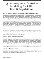
Cyclone efficiency as a function of particle size ratio is provided in Figure 9.6 (Lapple’s curve).
Solution:
Step 1. Determine the collection efficiency of the cyclone. Use Lapple’s method, which provides
collection efficiency and values from a graph relating efficiency to the ratio of average particle
diameter to the cut diameter. Again, the cut diameter is the particle diameter collected at 50%
efficiency (see Figure 9.6). Calculate the cut diameter using the Lapple method (Equation 9.19):
Determine the inlet width of the cyclone, B
c
. The permit application has established this cyclone
as conventional. The inlet width of a conventional cyclone is one fourth of the cyclone diameter:
Determine the value of p
p
– p. Because the particle density is much greater than the gas density,
p
p
– p can be assumed to be p
p
:
Calculate the cut diameter:
Figure 9.6 Lapple’s curve: cyclone efficiency vs. particle size ratio. (Adapted from USEPA-84/09, p 70.)

100
90
80
70
60
50
40
Collection efficiency, %
30
20
10
(0.1) 2 3 4 5 6 7 8 9 (1.0) 2 3 4 5 6 7 8 9 (10)
Particle size ratio, d
p
/(d
p
) cut
[] /[2 ( )]}0.5
cut c
dBnpp
ptvipg
= −{9µ π
B
c
===cyclone diameter/4 2.0/4 0.5 ft
ppp
pp
− == =2.75(62.4) 171.6 lb/ft
3
L1681_book.fm Page 227 Tuesday, October 5, 2004 10:51 AM

© 2005 by CRC Press LLC
228 ENVIRONMENTAL ENGINEER’S MATHEMATICS HANDBOOK
Calculate the ratio of average particle diameter to the cut diameter:
Determine the collection efficiency utilizing Lapple’s curve (see Figure 9.6):
Step 2. Calculate the required collection efficiency for the approval of the permit:

Step 3. Should the permit be approved? Because the collection efficiency of the cyclone is lower than
the collection efficiency required by the agency, the permit should not be approved.
9.4.6 Electrostatic Precipitator (ESP)
Electrostatic precipitators (ESPs) have been used as effective particulate-control devices for many
years. Usually used to remove small particles from moving gas streams at high collection efficien-
cies, ESPs are extensively used when dust emissions are less than 10 to 20 µm in size, with a
predominant portion in the submicron range (USEPA-81/10, p. 7-1). Widely used in power plants
for removing fly ash from the gases prior to discharge, electrostatic precipitators apply electrical
force to separate particles from the gas stream. A high voltage drop is established between elec-
trodes, and particles passing through the resulting electrical field acquire a charge. The charged
particles are attracted to and collected on an oppositely charged plate, and the cleaned gas flows
through the device. Periodically, the plates are cleaned by rapping to shake off the layer of dust
that accumulates; the dust is collected in hoppers at the bottom of the device (see Figure 9.7). ESPs
have the advantages of low operating costs; capability for operation in high-temperature applications
(to 1300°F); low-pressure drop; and extremely high particulate (coarse and fine) collection effi-
ciencies; however, they have the disadvantages of high capital costs and space requirements.
9.4.6.1 Collection Efficiency
According to USEPA-81/10, p. 7-9, ESP collection efficiency can be expressed by the following
two equations:
• Migration velocity equation
• Deutsch–Anderson equation
[] { /[2 ( )]}
cut c
dBnpp

ptvipg
= −9µ π
=×[(9)(1.21 10 )(0.5)/(2 )4.5(50)(171.6)
–5
π ]]
0.5
= 4.57 microns
d/[d ] 7.5/4.57 1.64
ppcut
==
η 72%=
µ [(inlet loading – outlet loading)/(inle= ttloading)](100)
= [(0.5 – 0.1)/(0.5)](100)
= 80%
L1681_book.fm Page 228 Tuesday, October 5, 2004 10:51 AM
© 2005 by CRC Press LLC
PARTICULATE EMISSION CONTROL 229
Particle migration velocity. The migration velocity w (sometimes referred to as the drift velocity)
represents the parameter at which a group of dust particles in a specific process can be collected
in a precipitator; it is usually based on empirical data. The migration velocity can be expressed in
terms of:
(9.20)
where
w = migration velocity
d
p
= diameter of the particle, microns
E
o
= strength of field in which particles are charged, volts per meter (represented by peak voltage)

E
p
= strength of field in which particles are collected, volts per meter (normally, the field close to
the collecting plates)
µ = viscosity of gas, pascal-seconds
Figure 9.7 Electrostatic precipitators. (From USEPA, Control Techniques for Gases and Particulates, 1971.)
to plates
Clean
gas out
Dirty
gas in
Dirty
gas in
Discharge
electrode (wire)
Clean
gas out
Collection
plate
High
voltage
to wires
(a)
Weights
Clean
gas out
Spray
Clean
gas out
Dirty

gas in
Dirty
gas in
Discharge
electrode
(wire)
(b)
Weights
wdEE µ)
po
=
p
/(4π
L1681_book.fm Page 229 Tuesday, October 5, 2004 10:51 AM
© 2005 by CRC Press LLC
230 ENVIRONMENTAL ENGINEER’S MATHEMATICS HANDBOOK
Migration velocity is quite sensitive to the voltage, as the presence of the electric field twice
in Equation 9.20 demonstrates. Therefore, the precipitator must be designed using the maximum
electric field for maximum collection efficiency. The migration velocity is also dependent on particle
size; larger particles are collected more easily than smaller ones.
Particle migration velocity can also be determined by the following equation:
(9.21)
where
w = migration velocity
q = particle charge (charges)
E
p
= strength of field in which particles are collected, volts per meter (normally, the field close to
the collecting plates)
µ = viscosity of gas, pascal-seconds

r = radius of the particle, microns
Deutsch–Anderson equation. This equation or derivatives thereof are used extensively through-
out the precipitator industry. Specifically, it has been used to determine the collection efficiency of
the precipitator under ideal conditions. Though scientifically valid, a number of operating param-
eters can cause the results to be in error by a factor of two of more. Therefore, this equation should
be used only for making preliminary estimates of precipitation collection efficiency. The simplest
form of the equation is:
(9.22)
where
η = fractional collection efficiency
A = collection surface area of the plates
Q = volumetric flow rate
w = drift velocity
9.4.6.2 Precipitator Example Calculations
Example 9.8
Problem:
A horizontal parallel-plate electrostatic precipitator consists of a single duct, 24 ft high and 20
ft deep, with an 11-in. plate-to-plate spacing. Given collection efficiency at a gas flow rate of 4200
actual cubic feet per minute (acfm), determine the bulk velocity of the gas, outlet loading, and drift
velocity of this electrostatic precipitator. Also calculate revised collection efficiency if the flow rate
and the plate spacing are changed (USEPA-84/09, p. 71).
Given:
Inlet loading = 2.82 gr/ft
3
(grains per cubic foot)
Collection efficiency at 4200 acfm = 88.2%
Increased (new) flow rate = 5400 acfm
New plate spacing = 9 in.
wqE/(µr)
p

= 4π
η = −1exp(–wA/Q)
L1681_book.fm Page 230 Tuesday, October 5, 2004 10:51 AM
© 2005 by CRC Press LLC
PARTICULATE EMISSION CONTROL 231
Solution:
Step 1. Calculate the bulk flow (throughout) velocity v. The equation for calculating throughput velocity
is
where
Q = volumetric flow rate
S = cross-sectional area through which the gas passes

Step 2. Calculate outlet loading. Remember that
Therefore,

Step 3. Calculate the drift velocity, which is the velocity at which the particle migrates toward the
collection electrode with the electrostatic precipitator. Recall that Equation 9.22, the Deut-
sch–Anderson equation, describes the collection efficiency of an electrostatic precipitator:
where
η = fractional collection efficiency
A = collection surface area of the plates
Q = volumetric flow rate
w = drift velocity
Calculate the collection surface area A. Remember that the particles will be collected on both
sides of the plate.
VQ/S=
VQ/S=
(4200)/[(11/12)(24)]=
191 ft/min=
3.2 ft/sec=

η (fractional) (inlet loading – outlet== lloading)/(inlet loading)
outlet loading inlet loading)(1 )= −( η
(2.82)(1 – 0.882)=
0.333 gr/ft
3
=
η = 1exp(–wA/Q)
A(2)(24)(20) 960 ft
2
==
L1681_book.fm Page 231 Tuesday, October 5, 2004 10:51 AM
© 2005 by CRC Press LLC