Vorticity and Vortex Dynamics 2011 Part 2 doc
Bạn đang xem bản rút gọn của tài liệu. Xem và tải ngay bản đầy đủ của tài liệu tại đây (877.59 KB, 50 trang )
40 2 Fundamental Processes in Fluid Motion
due to the Gauss theorem and (2.98a). Thus, there must be u
⊥1
= u
⊥2
and
hence ∇φ
1
= ∇φ
2
. This guarantees the uniqueness of the decomposition and
excludes any scalar potentials from u
⊥
. Moreover, (2.89a) and (2.98b) form a
well-posed Neumann problem for φ, of which the solution exists and is unique
up to an additive constant. Hence so does u
⊥
= u −∇φ. Collecting the earlier
results, we have (Chorin and Marsdon 1992)
Helmholtz–Hodge Decomposition Theorem. A vector field u on V
can be uniquely and orthogonally decomposed in the form u = ∇φ+u
⊥
,where
u
⊥
has zero divergence and is parallel to ∂V .
This result sharpens the Helmholtz decomposition (2.87) and is called
Helmholtz–Hodge decomposition. It is one of the key mathematic tools in ex-
amining the physical nature of various fluid-dynamics processes.
Note that from scalar φ one can further separate a harmonic function ψ
with ∇
2
ψ = 0, such that ∇ψ is also orthogonal to both ∇(φ−ψ)andu
⊥
.Thus,
strictly, u has a triple orthogonal decomposition. The harmonic part belongs
to neither compressing nor shearing processes, but is necessary for φ and ψ
to satisfy the orthogonality boundary conditions and thereby influences both.
For example, if a vorticity field ω has zero normal component on boundary so
that ω = ω
⊥
, there can be ∇×ω =(∇×ω)
⊥
if the former is not tangent to
the boundary. In this case we introduce a harmonic function χ, say, and write
∇×ω =(∇×ω)
⊥
+ ∇χ, (2.99)
where
∇
2
χ =0 in V, (2.100a)
∂χ
∂n
= n · (∇×ω)=(n ×∇) · ω on ∂V. (2.100b)
The second equality of (2.100b) implies that χ is not trivial once ω varies
along ∂V , of which the significant consequence will be analyzed in Sect. 2.4.3.
2.3.2 Integral Expression of Decomposed Vector Fields
In the special case where the Fourier transform applies, we have obtained the
explicit expressions of u
and u
⊥
in terms of a given u as seen from (2.96).
This local relation in the spectral space must be nonlocal in the physical
space after the inverse transform is performed. Indeed, comparing (2.87) with
identity (2.86), it is evident that if we set u = −∇
2
F then the Helmholtz
potentials in (2.87) are simply given by φ = −∇·F and ψ = ∇×F . Computing
these potentials for given u amounts to solving Poisson equations, and the
result must be nonlocal.
Without repeatedly mentioning, in what follows use will be frequently
made of the generalized Gauss theorem given in Appendix A.2.1. Let G(x)be
the fundamental solution of Poisson equation
2.3 Intrinsic Decompositions of Vector Fields 41
∇
2
G(x)=δ(x) (2.101)
in free space, which in n-dimensional space, n =2, 3, is known as
G(x)=
1
2π
log |x|, if n =2,
−
1
4π|x|
, if n =3.
(2.102)
The gradient of G will be often used:
∇G =
x
2(n − 1)π|x|
n
. (2.103)
Now assume u is given in a domain V and u = 0 outside V . We define a
vector F by
F (x)=−
V
G(x − x
)u(x
)dV
,
where dV
=dV (x
). On both sides we consider the Laplacian, which does
not act to functions of x
but to G(x − x
) only. By (2.101) we have
−∇
2
F =
V
δ(x −x
)u(x
)dV
=
u if x ∈ V,
0 if x /∈ V.
Thus, replacing u in identities (2.86) and (2.87) by F , and denoting the
gradient operator with respect to the integration variable x
by ∇
so that
∇G = −∇
G and ∇
2
G = ∇
2
G, we obtain, when x is in V ,
φ = −∇ · F = −
∇
G · u dV
=
V
Gϑ dV
−
∂V
Gn · u dS
, (2.104a)
ψ = ∇×F =
∇
G × u dV
= −
V
Gω dV +
∂V
Gn × u dS
, (2.104b)
where the second-line expressions were obtained by integration by parts.
When x is outside V , these integrals vanish. Therefore, we have constructed
a Helmholtz decomposition of u:
u = ∇φ + ∇×ψ for x ∈ V,
0 = ∇φ + ∇×ψ for x /∈ V.
For unbounded domain, the Helmholtz decomposition is still valid provided
that the integrals in (2.104) converge. This is the case if (ω,ϑ) vanish outside
42 2 Fundamental Processes in Fluid Motion
some finite region or decay sufficiently fast (Phillips 1933; Serrin 1959).
10
Therefore, (2.104) provides a constructive proof of the global existence of the
Helmholtz decomposition for any differentiable vector field. Moreover, (2.104)
indicates that the split vectors ∇φ and ∇×ψ canbeexpressedintermsof
dilatation and vorticity, respectively:
∇φ =
V
ϑ∇G dV
−
∂V
(n · u)∇G dS
, (2.105a)
∇×ψ =
V
ω ×∇G dV
−
∂V
(n × u) ×∇G dS
. (2.105b)
This result is the generalized Biot–Savart formulas to be discussed in detail in
Chap. 3. The formulas not only show the nonlocal nature of the decomposition
but also, via (2.103), tells how fast the influence of ω and ϑ at x
on the field
point x decays as |x − x
| increases.
It should be stressed that for bounded domain the earlier results only
provide one of all possible pairs of Helmholtz decomposition of u.Itdoes
not care any boundary condition for ∇φ and ∇×ψ. In order to obtain
the unique Helmholtz–Hodge decomposition, the simplest way is to solve the
scalar boundary-value problem (2.89a) and (2.98b). To see the structure of
the solution, we use Green’s identity
V
(G∇
2
φ − φ∇
2
G)dV =
∂V
G
∂φ
∂n
− φ
∂G
∂n
dS
along with (2.98b) to obtain
φ =
V
Gϑ dV −
∂V
Gn · u + φ
∂G
∂n
dS. (2.106)
Compared with (2.104a), we now have an additional surface integral with
unknown boundary value of φ. To remove this term we have to use a boundary-
geometry dependent Green’s function
G instead of G, which is the solution of
the problem
∇
2
G(x)=δ(x),
∂
G
∂n
=0 on ∂V. (2.107)
This gives a unique
∇
φ =
V
ϑ∇
G dV −
∂V
n · u∇
G dS, (2.108)
and hence u
⊥
= u −∇
φ is the unique transverse vector.
The Helmholtz–Hodge decomposition is also a powerful and rational tool
for analyzing numerically obtained vector fields, provided that effective meth-
ods able to extend operators gradient, curl, and divergence from differential
formulation to discrete data can be developed. For recent progress see, e.g.,
Tong et al. (2003).
10
For the asymptotic behavior of velocity field in unbounded domain see Sect. 3.2.3.
2.3 Intrinsic Decompositions of Vector Fields 43
2.3.3 Monge–Clebsch decomposition
So far we have been able to decompose a vector field into longitudinal and
transverse parts. It is desirable to seek a further intrinsic decomposition of
the transverse part into its two independent components. A classic approach
is to represent the solenoidal part of a vector, say v ≡ u −∇φ = ∇×ψ,by
two scalars explicitly, at least locally:
v = ∇ψ ×∇χ. (2.109)
The variables φ, ψ,andχ are known as Monge potentials (Truesdell 1954) or
Clebsch variables (Lamb 1932). For the proof of the local existence of ψ and χ,
the reader is referred to Phillips (1933). Then, since ∇×(ψ∇χ)=∇ψ ×∇χ,
for the Helmholtz vector potential of u we may set (Phillips 1933; Lagerstrom
1964)
ψ = ψ∇χ, (2.110)
or more symmetrically (Keller 1996),
ψ =
1
2
(ψ∇χ −χ∇ψ). (2.111)
Both ways cast the Helmholtz decomposition (2.87) to a special form
u = ∇φ + ∇ψ ×∇χ, (2.112)
where the vector stream function ψ is replaced by two scalar stream functions
ψ and χ. Accordingly, the vorticity is given by
ω = ∇×(∇ψ ×∇χ)
= ∇
2
χ∇ψ −∇
2
ψ∇χ +(∇χ ·∇)ψ − (∇ψ ·∇)χ. (2.113)
The Monge–Clebsch decomposition has proven useful in solving some vor-
tical flow problems (Keller 1998, 1999), but it is not as powerful as the
Helmholtz–Hodge decomposition since unlike the latter it may not exist glob-
ally. Thus, if one wishes ψ and χ satisfy boundary condition (2.98a) or
n · (∇ψ ×∇χ)=0 on ∂V (2.114)
and thereby produce a Helmholtz–Hodge decomposition, the problem may
not be solvable. Also note that neither (2.110) nor (2.111) satisfies the gauge
condition (2.88) although both contain only two independent variables.
Instead of the solenoidal part of u, one can also represent the vorticity ω
in the form of (2.109). In this case we set
u = ∇φ + v, v = λ∇µ, (2.115)
so that ω = ∇λ ×∇µ and ∇×(u − λ∇µ)=0. This is the original form of
the Monge decomposition, also called the Clebsch transformation (Lamb 1932;
Serrin 1959). But in general λ∇µ is not a solenoidal vector and (2.115) does
not represent any Helmholtz decomposition.
44 2 Fundamental Processes in Fluid Motion
2.3.4 Helical–Wave Decomposition
An entirely different approach to intrinsically decompose a transverse vector
and giving its two independent components clear physical meaning, free from
the mathematical limitation of Clebsch variables, can be inspired by observing
light waves. A light wave is a transverse wave and can be intrinsically split
into right- and left-polarized (helical) waves.
11
Mathematically, making this
splitting amounts to finding a complete set of intrinsic basis vectors, which
are mutually orthogonal in the sense of (2.90), and by which any transverse
vector can be orthogonally decomposed.
Recalling that the curl operator retains only the solenoidal part of a vector,
and observe that the sign of its eigenvalues may determine the right- and left-
polarity or handedness. We thus expect that the desired basis vectors should
be found from the eigenvectors of the curl. Indeed, denote the curl-eigenvalues
by λk, where λ = ±1 marks the polarity and k = |k| > 0 is the wave number
with k the wave vector. Then there is
Yoshida–Giga Theorem (Yoshida and Giga 1990). In a singly-connected
domain D, the solutions of the eigenvalue problem
∇×φ
λ
(k, x)=λkφ
λ
(k, x)inD,
n · φ
λ
(k, x)=0on∂D,
λ = ±1, (2.116)
exist and form a complete orthogonal set {φ
λ
(k, x)} to expand any transverse
vector field u
⊥
parallel to ∂D.
12
These φ
λ
s can only be found in complex vector space. Their orthogonality
(normalized) is expressed by
φ
λ
(k, x), φ
∗
µ
(k
, x) = δ
λµ
δ(k −k
),λ,µ= ±1, (2.117a)
k
φ
λi
(k, x)φ
λj
(k, x
)=δ
ij
δ(x − x
),λ= ±1, (2.117b)
where the asterisk means complex conjugate and repeated indices imply
summation. Using this basis to decompose a transverse vector is called the
helical-wave decomposition (HWD). For neatness we use ·, · to denote the
inner-product integral over the physical space, then the HWD of F
⊥
reads
11
A transverse vector, which can be constructed by vector product or curl operation,
is an axial vector or pseudovector. It is always associated with an antisymmetric
tensor (see Appendix A.1) and changes sign under a mirror reflection. And, like
polarized light, an axial vector is associated with certain polarity or handedness.A
true vector, also called polar vector, does not change sign by mirror reflection and
has no polarity. In an n-dimensional space the number of independent components
of a true vector must be n, but that of an axial vector is the number of the indepen-
dent components in its associated antisymmetric tensor, which is m = n(n−1)/2.
Thus, only in three-dimensional space there is m=n, but in two-dimensional space
an axial vector has only one independent variable (e.g., Lugt 1996).
12
Additional condition is necessary in a multiple-connected domain.
2.3 Intrinsic Decompositions of Vector Fields 45
F
⊥
(x,t)=
k
F
λ
(k,t)φ
λ
(k, x), (2.118a)
F
λ
(k,t)=F (x,t), φ
∗
λ
(k, x). (2.118b)
Note that F −F
⊥
, φ
λ
=0.
For example, for an incompressible flow with u
n
= ω
n
=0on∂D, one can
expand
u(x,t)=
k,λ
u
λ
(k,t)φ
λ
(k, x), ω(x,t)=
k,λ
λu
λ
(k,t)φ
λ
(k, x). (2.119)
Here the term-by-term curl operation on the infinite series converges. However,
as seen from (2.99) and (2.100), although ∇×ω is solenoidal, only (∇×ω)
⊥
can
have HWD expansion on which the term-by-term curl operation converges.
Therefore, the result is
∇×ω =
k,λ
λ
2
u
λ
φ
λ
+ ∇χ, (2.120)
where χ is determined by (2.100).
The specific form of HWD basis depends solely on the domain shape. In
a periodic box (2.116) is simplified to
ik ×φ
λ
(k, x)=λkφ
λ
(k, x),
from which the normalized HWD eigenvectors can be easily found (Moses
1971, Lesieur 1990):
φ
λ
(k, x)=h
λ
(k)e
ik·x
,
h
λ
(k)=
1
√
2
[e
1
(k)+iλe
2
(k)],
(2.121)
where λ = ±1, and e
1
(k), e
2
(k), and k/k form a right-hand Cartesian triad.
In this case (2.117a) is simplified to
h
λ
(k) ·h
∗
µ
(k)=δ
λµ
. (2.122)
If the Cartesian triad is so chosen such that k = ke
z
, then
φ
λx
(k, x)=
1
√
2
cos kz, φ
λy
(k, x)=−
λ
√
2
sin kz, φ
λz
(k, x)=0. (2.123)
Therefore, as we move along the z-axis, the locus of the tip of φ
λ
(k, x) will be
a left-handed (or right-handed) helix if λ = 1 (or −1), having a pitch equal to
wavelength 2π/k, see Fig. 2.7. In other words, each eigenmode with nonzero
eigenvalue is a helical wave. This explains the name HWD. A combined use
of the Helmholtz–Hodge and HWD decompositions permits splitting a vector
intrinsically to its finest building blocks.
46 2 Fundamental Processes in Fluid Motion
k
Fig. 2.7. A helical wave
The simple Fourier HWD basis cannot be applied to domains other than
periodic boxes. To go beyond this limitation, we notice that the curl of (2.116)
along with itself leads to a vector Helmholtz equation
∇
2
φ
λ
+ k
2
φ
λ
= 0. (2.124)
Unlike (2.116), now the three component equations are decoupled, each rep-
resenting a Sturm–Liouville problem. Then in principle one can use the
Helmholtz vectors to construct the HWD bases. Since a transverse vector
field depends on only two scalar fields, say ψ and χ, a simplification may
occur if both scalars are solutions of the scalar Helmholtz equation
∇
2
ψ + k
2
ψ =0. (2.125)
Morse and Feshbach (1953, pp. 1764–1766) have shown that this can indeed
be realized in and only in Cartesian, cylindrical, spherical, and conical coor-
dinates. Specifically, a transverse solutions (not normalized) of (2.124) can be
written as
a
⊥
= M + N , M = ∇×(ewψ), N =
1
k
∇×∇×(ewχ),
where e can be three Cartesian unit vectors, the unit vector along the axis
in cylindrical coordinates, or that along the radial direction in spherical and
conical coordinates, but none other. the scalar w in the first two cases is 1,
while in the others is the radius r. In particular, when ψ = χ there is
∇×(M + λN )=λk(M + λN );
thus, one can write down the HWD basic vector (not normalized)
φ
λ
= ∇×(ewψ)+
λ
k
∇×∇×(ewψ). (2.126)
Chandrasekhar and Kendal (1957) have given the HWD basis in terms of
spherical coordinates. For vorticity dynamics the basis in terms of cylindrical
coordinates (r, θ, z) is of interest. Assume that along the z-axis we can impose
periodic boundary condition. Then a scalar Helmholtz solution that is regular
2.3 Intrinsic Decompositions of Vector Fields 47
at r =0is
ψ = J
m
(βr)e
i(mθ+k
z
z)
,k
z
=
πn
L
,
β
2
= k
2
− k
2
z
,m=0, 1, 2, , n= ±1, ±2, ,
where J
m
(βr) are Bessel functions of the first kind. Substituting this ψ into
(2.126) and multiplying the result by a constant iα
λ
(λ, n) ≡ iλk/k
z
, we obtain
φ
λ
r
=
J
m+1
(βr) −
m
βr
(1 + α
λ
)J
m
(βr)
e
i(mθ+k
z
z)
,
φ
λ
θ
=i
α
λ
J
m+1
(βr) −
λm
βr
(1 + α
λ
)J
m
(βr)
e
i(mθ+k
z
z)
,
φ
λ
z
=i
β
k
z
J
m
(βr)e
i(mθ+k
z
z)
.
(2.127)
This result has been applied to vortex-core dynamics, see Sect. 8.1.4. The
HWD has also found important applications in the analysis of turbulent
cascade process; e.g., Waleffe (1992, 1993); Chen et al. (2003), and refer-
ences therein. For a bounded domain of arbitrary shape, finding the curl-
eigenvectors is not an easy task and requires special numerical algorithms
(e.g., Boulmezaoud and Amari 2000).
2.3.5 Tensor Potentials
Before closing this section we take a further look at the Helmholtz potentials.
Return to the Cauchy motion equation (2.44) and denote
f
s
≡∇·T = lim
V →0
1
V
∂V
t dS
, (2.128)
which is the resultant surface force per unit volume and contains most of the
kinetic properties of flows. Assume we have decomposed f
s
to
f
s
= −∇Φ + ∇×Ψ , ∇·Ψ =0. (2.129)
Observe that
−Φ
,i
+
ijk
Ψ
k,j
= −(Φδ
ji
+
jik
Ψ
k
)
,j
,
where
jik
Ψ
k
≡ Ψ
ji
= −Ψ
ij
(2.130)
is an antisymmetric tensor. Thus, (2.129) can be written as
f
s
= ∇·
T,
T
ij
≡−(Φδ
ij
+ Ψ
ij
). (2.131)
As a generalization of the concept of scalar and vector potentials φ and ψ in
(2.87), we may view the stress tensor T and the tensor
T as tensor potentials
48 2 Fundamental Processes in Fluid Motion
of f
s
. Obviously there must be ∇·(T −
T)=0. Any other tensor, say T
,can
also be a tensor potential of f
s
provided that T −T
is divergenceless. Thus,
while for Newtonian fluid the stress tensor T is uniquely given by (2.45), f
s
has infinitely many tensor potentials, among which the above
T with only
three independent components is the simplest one. We call it the Helmholtz
tensor potential of f
s
.
The value of introducing the Helmholtz potential lies in the fact that in
(2.44) the six-component T plays a role only through its divergence. Therefore,
once the expression of
T (or the Helmholtz potentials Φ and Ψ ) is known, in
the local momentum balance T can well be replaced by the simpler
T.Thus
we call
T the reduced stress tensor. However, on any open surface
T produces
a reduced surface force
tt
t
(x, n)=n ·
T(x)=−Φn + n × Ψ , (2.132)
which is generically different from the full surface force t given by (2.43). It is
here that the extra part of T cannot be ignored. Nevertheless, the replacement
of t by
tt
t
is feasible when one considers the volume integral of f
s
:
V
f
s
dV =
∂V
t dS =
∂V
tt
t
dS (2.133)
due to the Gauss theorem.
Remarks:
1. We know the divergence of any differentiable tensor of rank 2 is a vector.
Now since for any vector field one can always find its Helmholtz potentials
as proven by the Helmholtz–Hodge theorem, we see the inverse is also true.
2. Because the Helmholtz decomposition is a global operation, in applica-
tions the replacement of (T, t)by(
T,
tt
t
) is convenient only when f
s
has a
natural Helmholtz decomposition, as in the kinematic case of (2.86). This
important situation also occurs in dynamics as will be seen in the Sect. 2.4.
3. The body force ρf in (2.44) can also be expressed as the divergence of
a tensor potential. But this in no ways means that one may cast any
body force to a resultant surface force. Whether a force is a body force
or surface force should be judged by physics rather than mathematics; a
surface force is caused by internal contact interaction of the fluid.
2.4 Splitting and Coupling of Fundamental Processes
Having reviewed the basic principles of Newtonian fluid dynamics and intro-
duced the intrinsic decomposition of vector fields, we can now gain a deeper
insight into the roles of compressing and shearing processes in the kinematics
and dynamics of a Newtonian fluid. Our main concern is the splitting and
coupling of the two processes in the Navier–Stokes equation (2.47). As just
2.4 Splitting and Coupling of Fundamental Processes 49
remarked, the splitting will be convenient when a natural Helmholtz decom-
position manifests itself from (2.47). Remarkably, this is the case as long as µ
is constant. By using (2.86) we have
2∇·D = ∇ϑ + ∇
2
u =2∇ϑ −∇×ω,
so (2.47) immediately yields a natural Helmholtz decomposition of the total
body force (inertial plus external) as pointed out by Truesdell (1954):
ρ
Du
Dt
− ρf = −∇Π −∇×(µω), (2.134)
where
Π ≡ p − (λ +2µ)ϑ (2.135)
consists of the pressure and a viscous contribution of dilatation. The appear-
ance of pressure changes the dynamic measure of the compressing process to
the isotropic part of T (per unit volume), which is Π; and the dynamic mea-
sure of the shearing process remains to be the vorticity ω (multiplied by the
shear viscosity).
13
The elegance of (2.134) lies in the fact that Π and ω have only three inde-
pendent components, and three more independent components in the strain-
rate tensor D do not appear. This fact deserves a systematic examination of
its physical root and consequences, which is the topics of this section.
2.4.1 Triple Decomposition of Strain Rate and Velocity Gradient
According to our discussion on tensor potentials of a vector in Sect. 2.3.5
and the Cauchy motion equation (2.44), the natural Helmholtz decomposi-
tion in (2.134) implies that there must be a natural algebraic decomposi-
tion of the stress tensor T for Newtonian fluid, able to explicitly reveal the
Helmholtz tensor-potential part of T. This, by the Cauchy–Poisson equation
(2.45), in turn implies that the desired algebraic decomposition must exist
in the strain-rate tensor D. Therefore, we return to kinematics. Unlike the
classic symmetric-antisymmetric decomposition (2.18), we now consider the
intrinsic constituents of D in terms of fundamental processes. The result is
simple, but has much more consequences than merely for rederiving (2.134).
Since D
T
= D but Ω
T
= −Ω, we may write
(∇u)
T
= D −Ω + ϑI − ϑI,
13
The dynamic measure of compressing process per unit mass may switch to other
scalars, see later.
50 2 Fundamental Processes in Fluid Motion
so that by (2.27) there is an intrinsic triple decomposition of D and ∇u (Wu
and Wu 1996):
D = ϑI + Ω −B, (2.136a)
∇u = ϑI +2Ω − B. (2.136b)
Thus, the velocity gradient and rate of strain consist of a uniform expan-
sion/compression, a rotation, and a surface deformation. Here, B has most
complicated structure among the three tensors on the right-hand side, and
needs a further examination.
As seen from (2.26) and (2.29), the primary appearance of B is in the form
of n ·B for the rate of change of a surface element dS = n dS, which involves
the kinematics on the surface only. Denoting the tangent components of any
vector by suffix π, it can then be shown that (Appendix A.3.2)
n · B =(∇
π
· u)n −(∇
π
u
n
+ u ·K), (2.137)
where
K ≡−∇
π
n (2.138)
is the symmetric curvature tensor of dS consisting of three independent tan-
gent components. Then (2.137) can be written as
n · B =
n
dS
D
Dt
dS +
Dn
Dt
= nr
s
+ W × n, (2.139)
where r
s
is the rate of change of the surface area and W (x,t) is the angular
velocity of n, expressed solely in terms of the velocity and geometry of the
surface (the normal component of W is simply W
n
= ω
n
/2):
r
s
= ∇
π
· u = ϑ −u
n,n
(2.140a)
W
π
= −n × (∇
π
u
n
+ u ·K). (2.140b)
Return now to the triple decomposition (2.136). As a special case and
a fundamental application, we consider its form on an arbitrary material
boundary B with unit normal n and velocity u = b. The resulting kinematic
knowledge (Wu et al. 2005c) is indispensible in studying any fluid-boundary
interactions. Due to the adherence, we may write
∇u = n(n ·∇u)+∇
π
u = n(n ·∇u)+∇
π
b on B.
Since (2.136b) gives
n ·∇u = nϑ + ω × n −n · B,
we obtain
∇u = nnϑ + n(ω ×n) − n(n · B)+∇
π
b on B. (2.141)
2.4 Splitting and Coupling of Fundamental Processes 51
Here, the tensor ∇
π
b depends solely on the motion and deformation of B but
independent of the flow. To see the implication of (2.141), we first assume B
is rigid to which our frame of reference can be attached, so the last two terms
vanish:
∇u = nnϑ + n(ω ×n).
Then, taking the symmetric part immediately yields the Caswell formula
(Caswell 1967):
2D =2nnϑ + n(ω ×n)+(ω ×n)n, (2.142)
where by (2.140a) ϑ can be replaced by u
n,n
since r
s
=0.
We now extend (2.142) to an arbitrary deformable surface B (to which no
frame of reference can be attached). For this purpose we only need to treat
the tensor ∇
π
b in (2.141). In general, it consists of a tangent–tangent tensor
(∇
π
b)
π
and a tangent–normal tensor
(∇
π
b · n)n =(∇
π
b
n
− b ·∇
π
n)n = −(W × n)n
due to (2.138) and (2.140b). Substituting these into (2.141) and using (2.139)
to express n ·B, we obtain a general kinematic formula:
∇u = nnu
n,n
+ n(ω × n) − [n(W ×n)+(W × n)n]+(∇
π
b)
π
. (2.143)
Note that r
s
in the normal–normal component is canceled. Then, let S and A
be the symmetric and antisymmetric parts of (∇
π
b)
π
, from (2.143) it follows
that
2D =2nnu
n,n
+ n(ω
r
× n)+(ω
r
× n)n +2S, (2.144)
2Ω = n(ω ×n) −(ω × n)n +2A, (2.145)
where ω
r
≡ ω−2W is the relative vorticity with n·ω
r
= 0, see (2.69). Tensor S
has three independent components and can be called surface-stretching tensor.
In contrast, A has only one independent component, which must be ω
n
. Note
that on a rigid boundary (2.144) reduces to (2.142), but viewed in a frame of
reference fixed in the space.
The generalized Caswell formula (2.144) contains the key kinematics on
an arbitrary boundary B. It represents an intrinsic decomposition of D with
respect to one normal (N) and two tangent (T) directions, along with their
respective physical causes. Namely: the N–N component caused by the normal
gradient of normal velocity; the N–T and T–N components caused by the rela-
tive vorticity; and the T–T components caused by the surface flexibility. With
known b(x,t)-distribution and surface geometry, (2.143) and (2.144) express
a basic fact that the motion and deformation of a fluid element neighboring B
are described by only three independent components of velocity derivatives.
The form of (2.144) suggests a convenient curvilinear orthonormal basis
(e
1
, e
2
,
nn
n
)onB.Lete
2
be along ω
r
,
nn
n
= −n (towards fluid), and hence e
1
is
52 2 Fundamental Processes in Fluid Motion
n
t
p
3
p
1
w
r
∂B
Fig. 2.8. Principal directions of the strain-rate tensor on a rigid boundary
along ω
r
×
nn
n
. It will be seen below (Sect.2.4.2) that for Newtonian fluid e
1
is the direction of shear stress τ ; thus we call this frame the τ-frame. Then
(2.144) reads
{D
ij
} =
S
11
S
12
ω
r
/2
S
12
r
s
− S
11
0
ω
r
/20u
n,n
. (2.146)
We have seen in Sect. 2.1.2 that the first and third eigenvalues λ
1,3
and
associated principal directions of D reflect the maximum stretching/shrinking
rates and directions, respectively. On a boundary B they have dominant effect
on the near-boundary flow structures and their stability. Let θ
1,3
be the angles
between the stretching/shrinking principal axes and e
1
of the τ -frame. If B
is rigid with S = 0 and if the flow is incompressible, from (2.146) it follows
at once that λ
1,3
= ±ω
r
/2, λ
2
=0,andθ
1,3
= ±45
◦
, as sketched in Fig. 2.8.
But the situation can be very different if B is deformable, as demonstrated by
Wu et al. (2005c).
2.4.2 Triple Decomposition of Stress Tensor and Dissipation
We move on to dynamics. Substituting (2.136a) into (2.45) immediately leads
to a triple decomposition of the stress tensor
T = −ΠI +2µΩ −2µB, (2.147)
where Π is defined by (2.135). Then since by (2.34b) µB is a trace-free
tensor, the first two terms on the right-hand side of (2.147) form the nat-
ural Helmholtz tensor potential of the surface force. In other words, for flow
with constant µ, the surface deformation process does not affect the local
2.4 Splitting and Coupling of Fundamental Processes 53
momentum balance (Wu and Wu 1993). This explains the origin of (2.134)
and permits introducing the reduced stress tensor and reduced surface stress
solely in terms of compressing and shearing processes:
T = −ΠI +2µΩ, (2.148)
tt
t
= n ·
T = −Πn + µω ×n. (2.149)
The conceptual simplification brought by
T can also lead to significant compu-
tational benefit. For example, Eraslan et al. (1983) have developed a Navier–
Stokes solver where some components of T were found never useful and hence
simply dropped. Consequently, for incompressible flow the solver reached a
big saving of CPU in stress computation.
Evidently, although for constant µ the surface-deformation stress does not
contribute to the differential momentum equation nor integrated surface force
over a closed boundary, it must show up in more general circumstances. Here
we consider two simple examples; in Sect. 4.3.2 we shall see the crucial role of
the surface-deformation stress in free-surface flow.
First, on any surface element of unit area in the fluid or at its boundary,
we have a triple decomposition of the surface force:
t =
tt
t
+ t
s
, t
s
= −2µn ·B = −2µ(nr
s
+ W × n), (2.150)
where t
s
is the viscous resistance of the fluid surface to its motion and defor-
mation, which has both normal and tangent components. Thus, denote the
orthogonal decomposition of the stress by t = −
Πn+τ , by (2.135) the general
normal and tangent components are
Π = Π +2µr
s
= p −λϑ −2µu
n,n
, (2.151a)
τ = µω
r
× n, ω
r
= ω −2W . (2.151b)
On a solid wall τ
w
= −τ is the skin-friction stress, always determined by
the relative vorticity. Note that t
s
= 0 only if the surface performs uniform
translation; even a rigid rotation will cause a nonzero t
s
due to the viscous
resistance to the variation of n.
Second, using the generalized Stokes theorem (A.17) and its corollary
(A.26), from (2.150) and (2.29) we find the general formulas for integrated
force and moment due to t
s
on an open surface S with boundary loop C:
S
t
s
dS =2µ
C
dx × u, (2.152a)
S
x × t
s
dS =2µ
C
x × (dx × u) −2µ
S
n × u dS. (2.152b)
In particular, on a closed boundary ∂V of a fluid volume V , by the generalized
Gauss theorem (A.14), the total moment due to t
s
is proportional to the total
54 2 Fundamental Processes in Fluid Motion
vorticity in V (Wu and Wu 1993):
∂V
x × t
s
dS = −2µ
∂V
n × u dS = −2µ
V
ω dV. (2.153)
Corresponding to (2.147), a triple decomposition can also be made for the
dissipation Φ, which brings some simplification too. We start from a kinematic
identity (cf. Truesdell 1954)
D : D = ϑ
2
+
1
2
ω
2
−∇·(B · u), (2.154)
where ω
2
≡|ω|
2
is called the enstrophy. Thus, for constant µ, (2.54) yields
the triple decomposition of dissipation rate:
Φ =(λ +2µ)ϑ
2
+ µω
2
−∇·(2µB · u). (2.155)
Once again, the role of the three viscous constituents of stress tensor is
explicitly revealed. Note that the B-part of Φ can be either positive or nega-
tive. More interestingly, we have
t · u = −Πn · u + µω · (n × u) −n · (2µB · u);
substituting this and (2.155) into (2.52), we see that the B-part of Φ and that
of t · u are canceled. Explicitly, at each point the work rate per unit volume
done by t
s
is
w
s
≡ lim
V→0
1
V
∂V
t
s
· u dS = −∇ ·(2µB ·u),
precisely the last term of (2.155), say Φ
s
. Therefore, the work done by t
s
does
not influence the change of kinetic energy but always directly dissipated into
heat (Wu et al. 1999a). Hence, instead of (2.52) and (2.53) we can simply
write
d
dt
V
ρ
1
2
q
2
dv =
V
(ρf · u + pϑ −
Φ)dv +
∂V
tt
t
· u dS, (2.156a)
ρ
D
Dt
1
2
q
2
= ρf · u + pϑ + ∇·(
T · u) −
Φ, (2.156b)
where
T and
tt
t
are given by (2.148) and (2.149), and
Φ ≡ Φ − Φ
s
=(λ +2µ)ϑ
2
+ µω
2
≥ 0 (2.157)
is the reduced dissipation, again due only to compressing and shearing processes.
Wu et al. (1999a) notice that the characteristic distribution of scalars ϑ
2
, ω
2
,
and Φ
s
in (2.157) may serve as good indicators for identifying different struc-
tures in a complex high Reynolds-number flow. However, it should be warned
2.4 Splitting and Coupling of Fundamental Processes 55
that it is the full dissipation Φ rather than
Φ that causes the entropy pro-
duction in (2.61). Otherwise a fluid making a solid-like rotation would have a
dissipation µω
2
, which is of course incorrect.
Finally, for constant µ, from (2.155) the total dissipation over a volume V
is
V
Φ dV =
V
[(λ +2µ)ϑ
2
+ µω
2
]dV +
∂V
t
s
· u dS. (2.158)
This result generalizes the Bobyleff–Forsythe formula (Serrin 1959) for im-
compressible flow:
V
Φ dV = µ
V
ω
2
dV +2µ
∂V
u ·∇u ·n dS. (2.159)
If ∂V extends to infinity where the fluid is at rest, then only the reduced
dissipation
Φ contributes to the total full dissipation.
So far we have assumed a constant µ. More generally, with µ = µ(T )
the natural Helmholtz decomposition of the momentum equation (2.134) no
longer exactly holds. Rather, there will be (Wu and Wu 1998)
ρ
Du
Dt
− ρf = −∇Π −∇×(µω) − 2∇µ ·B, (2.160a)
where B is the surface strain rate tensor. Here, the viscosity gradient can be
cast to
−∇µ =
S
µ
Pr
h
q with S
µ
≡
d log µ
d log T
, (2.160b)
where h = c
p
T is the enthalpy and q = −κ∇T the heat flux. Both the Prandtl
number Pr = µc
p
/κ and S
µ
are of O(1). Because q is along the normal of
isothermal surfaces, the extra term in (2.160a) is proportional to the viscous
resistance of isothermal surfaces to their deformation. In most cases this effect
is small.
2.4.3 Internal and Boundary Coupling of Fundamental Processes
For vorticity dynamics (and sometimes “compressing dynamics” as well), the
Navier–Stokes equation expressed for unit mass is more useful than that for
unit volume. But, once the fluid density is a variable, such an equation with
constant µ,
Du
Dt
= f −
1
ρ
∇Π − ν∇×ω, (2.161)
where ν = µ/ρ is the kinematic viscosity, is no longer a natural Helmholtz
decomposition. To discover the underlying physics of the two fundamental
processes and their coupling most clearly, we need a different decomposition
to maximally reveal the natural potential and solenoidal parts.
56 2 Fundamental Processes in Fluid Motion
First, on the left-hand side of (2.161) it is the nonlinear advective accel-
eration u ·∇u that causes all kinematic complexity of fluid motion, never
encountered in solid mechanics. Thus we decompose it first. Write
∇u = ∇u − (∇u)
T
+(∇u)
T
=2Ω +(∇u)
T
,
such that
2u · Ω = ω ×u, u · (∇u)
T
= ∇u ·u.
Then (2.11) is cast to the vorticity form, very important in vorticity and
vortex dynamics:
Du
Dt
=
∂u
∂t
+ ω × u + ∇
1
2
q
2
,q≡|u|. (2.162)
Therefore, the advective acceleration consists of two parts. One is the gradient
of kinetic energy, evidently a longitudinal process, implying that the acceler-
ation increases as fluid particles move toward higher kinetic-energy region.
The other is the Lamb vector ω × u already encountered in (2.85), which
is analogous to the Coriolis force observed in a rotating frame of reference
(see Sect. 12.1.1) and drives the particles move around the vorticity direction.
Generically ω ×u is neither solenoidal nor irrotational, and hence appears in
the evolution of both longitudinal and transverse processes.
Next, on the right-hand side of (2.161) there is an inviscid term −∇p/ρ,
which by (2.64) equals −∇h + T ∇s, where ∇h is also a natural longitudi-
nal process. Thus, (2.161) can be cast to the Crocco–Vazsonyi equation (its
inviscid version is the Crocco equation ):
∂u
∂t
+ ω × u − T∇s = f −∇H + η, (2.163)
where H is the total enthalpy defined in (2.63), and
η ≡
1
ρ
∇·V =
1
ρ
∇[(λ +2µ)ϑ] −ν∇×ω +
2
ρ
∇µ · D (2.164)
collects all viscous forces including variable µ. We may introduce a constant
averaged kinematic shear viscosity ν
0
and write η = η
−ν
0
∇×ω to separate
a basic viscous force due to vorticity diffusion, so that on the right-hand side
of (2.163) an explicit Helmholtz decomposition is recovered. The extra term
η
originates from compressibility and thermodynamics, which in most cases
is negligible. Therefore, the main complexity of (2.163) lies in its inviscid
nonlinear term called generalized Lamb vector:
L ≡ ω × u −T ∇s, (2.165)
which is usually dominated by the Lamb vector ω × u.
Now, in order to examine to what degree the two fundamental processes
can be split and how they are coupled, we assume the external body force
2.4 Splitting and Coupling of Fundamental Processes 57
does not exist (to be discussed in Sects. 3.6.2, 4.1.1, and Chap. 12), and take
the curl and divergence of (2.163). Since ν
0
∇×ω is divergence-free, this yields
∂ω
∂t
− ν
0
∇
2
ω = −∇× (L −η
), (2.166)
∂ϑ
∂t
+ ∇
2
H = −∇ · (L − η
). (2.167)
While (2.166) represents the general vorticity transport equation which char-
acterizes all transverse interactions, (2.167) characterizes all longitudinal
interactions and suggests that the viscous effect is much weaker than that
in (2.166). Because the Helmholtz decomposition is a linear operation, the
nonlinearity in L −η
in both equations makes the coupling of both processes
inevitable. It is their intersection.
For weakly compressible flow the entropy gradient can be neglected and ν
is nearly constant. Then (2.166) is reduced to the classic Helmholtz equation
for the vorticity to be studied in depth in this book:
∂ω
∂t
+ ∇×(ω × u) − ν∇
2
ω = 0, (2.168)
where the solenoidal part of the Lamb vector ω ×u is the only nonlinear term.
Meanwhile, under the same condition, (2.167) is reduced to
∂ϑ
∂t
+ ∇
2
H + ∇·(ω × u)=0, (2.169)
where the potential part of the Lamb vector ω × u appears. As a scalar
equation, the spatial structure of (2.169) is simpler than (2.168); but we have
to express one of the two scalars ϑ and H by the other, which complicates
the final form of (2.169). The result is an advective wave equation for the
total enthalpy H obtained by Howe (1975, 1998, 2003), with the Lamb vector
and entropy variation being the source of the wave. We illustrate the Howe
equation for inviscid homentropic flow. Multiplying the inviscid version of
(2.163) by ρ and taking divergence, we have
∇·
ρ
∂u
∂t
+ ∇·(ρ∇H)=−∇ · (ρω ×u).
Here, using (2.40) and the inviscid version of (2.65), there is
∇·
ρ
∂u
∂t
= ∇ρ ·
∂u
∂t
− ρ
∂
∂t
Dlnρ
Dt
= −ρ
D
Dt
∂ ln ρ
∂t
= −ρ
D
Dt
1
ρc
2
∂p
∂t
= −ρ
D
Dt
1
c
2
DH
Dt
,
58 2 Fundamental Processes in Fluid Motion
where c =(dp/dρ)
1/2
s
is the speed of sound. Therefore, it follows that (Howe,
2003)
D
Dt
1
c
2
D
Dt
−
1
ρ
∇·(ρ∇)
H =
1
ρ
∇·(ρω × u). (2.170)
In its most general form (Howe 1998), the Howe equation governs almost
all compressing processes and could be solved jointly with the vorticity trans-
port equation (2.166). But its main application is on the sound generated
by unsteady vorticity field, known as vortex sound named by Powell (1961,
1964), who studied this topic extensively under far-field approximation (see
the review of Powell (1995)). By using singular perturbation to match the far-
field and near-field solutions, Crow (1970a) was the first to prove rigorously
that the principal source of sound at low Mach numbers is the divergence
of the Lamb vector. In aeroacoustics, the variable describing the sound field
in a flow can be the fluctuating part of p, ρ, etc. but it has been found
that the most appropriate one is the disturbance total enthalpy H (Howe
1975; Doak 1998). Hence, (2.170) reveals that in a homentropic flow the mov-
ing vorticity is the only source of sound, or sound is a byproduct of vortex
motion.
In particular, at low Mach numbers with |u|/c 1, c and ρ in (2.170) can
be replaced by their constant mean values c
0
and ρ
0
, so that the equation is
reduced to the classic linear wave equation and can be solved by using the
Green’s function method. In this case the sound-wave length λ is generically
much larger than the scale of the moving vortices, so that to an observer at
a far-field point x the emission-time difference at different points y in the
source region is negligible: one has r = |x − y||x|. Then a general result
of interest is that the far-field acoustic pressure p
depends linearly on the
unsteady vorticity alone (M¨ohring 1978, Kambe et al. 1993, Powell 1994):
p
(x,t)=
ρ
0
β
i
β
j
4πc
2
0
x
∂
3
∂t
3
1
3
y
i
(y × ω)
j
(t − x/c
0
)d
3
y, (2.171)
where x = |x|, β
i
= x
i
/x is the directional cosine of x in the observation
direction, and the integrand is estimated at an earlier time t − x/c
0
.
The earlier coupling between the two processes dominated by the nonlinear
Lamb vector is inviscid in nature. It no longer exists on a solid boundary ∂B
with known motion or at rest. Due to the acceleration adherence (2.70), the
left-hand side of (2.161) is known, or simply vanishes in the frame of reference
fixed to the solid boundary. However, there appears a different type of viscous
boundary coupling of which the effect may also reach the interior of the flow
field. To illustrate the situation in its simplest circumstance, assume the flow
is incompressible and the solid wall is at rest. Then the momentum balance
implies
∇p + µ∇×ω = 0 on ∂B,
2.4 Splitting and Coupling of Fundamental Processes 59
so that
n ×∇p = −µn × (∇×ω), (2.172a)
n ·∇p = −µ(n ×∇) ·ω. (2.172b)
This pair of equations, especially (2.172a), contain rich physical and mathe-
matical information relevant to vorticity dynamics and will be fully explored
later. The absence of advection makes the coupling linear and hence a series
of formally analytical results are possible.
From the preceding analysis we may also summarize the involvement
of thermodynamics in dynamic processes, which can be both inviscid and
viscous. The viscous involvement of thermodynamics has been encountered
in (2.160). Inviscidly, it appears in the generalized Lamb vector (2.165). If
the flow is baroclinic, i.e., with more than one independent thermodynamic
variables, thermodynamics enters both compressing and shearing processes
through (p, ρ) in (2.161), or through (T,s) in (2.163). Two independent vari-
ables determine a surface with a normal direction; and in a baroclinic flow
this normal is ∇ρ ×∇p or ∇T ×∇s. In contrast, if the flow is barotropic, i.e.,
with only one independent thermodynamic variables so that ∇T ×∇s =0,the
inviscid coupling of thermodynamics and dynamics occurs only in compressing
process. For more discussion see Sects. 3.6.2 and 4.1.2 later.
2.4.4 Incompressible Potential Flow
In the context of Helmholtz–Hodge decomposition we have seen that a scalar
function χ with ∇
2
χ = 0 is necessary, and in general at large Re a big portion
of a viscous flow field can be irrotational. It is appropriate here to briefly
review some basic issues of incompressible potential flow.
Consider an externally unbounded fluid domain V
f
which is at rest at
infinity and in which a moving body B causes a single-valued or acyclic (or
noncirculatory) velocity potential φ,
14
which is solved from the kinematic
problem
∇
2
φ =0 in V
f
, (2.173a)
∂φ
∂n
= n · b on ∂B, φ → 0as|x| = r →∞, (2.173b)
where b is the velocity of ∂B. It is known that the far-field asymptotic behavior
of such a φ and u is
φ = −
A · n
r
n−1
+ , u = ∇φ =
n(A · n)n − A
r
n
+ , (2.174a,b)
14
A single-valued potential cannot have discontinuity, and hence excludes any vor-
tex sheet, across which a loop going once will have nonzero circulation, see (4.128)
and Fig. 4.19 of Sect. 4.4.
60 2 Fundamental Processes in Fluid Motion
where n =2, 3 is the space dimensions, n = x/r,andA depends on the body
shape and velocity.
First, by (2.173), the total kinetic energy of the flow is
K =
ρ
2
V
f
∇φ ·∇φ dV =
ρ
2
V
f
∇·(φ∇φ)dV =
ρ
2
∂B
φn · b dS. (2.175)
Thus, the flow has no memory on its history but completely depends on the
current motion of boundary. Since K = 0 implies ∇φ = 0 everywhere, if ∂V
f
is suddenly brought to rest then the entire flow stops instantaneously, which
is evidently unrealistic. In reality a fluid flow without moving boundary must
be vortical and/or compressible.
If one adds any disturbance u
to the velocity field with kinetic energy
K
> 0, such that u
1
= ∇φ + u
,andifu
· n =0on∂V
f
, then
K
1
=
ρ
2
V
f
(∇φ + u
) · (∇φ + u
)dV
= K + K
+ ρ
∂V
f
n · u
φ dS = K + K
>K. (2.176)
This is the famous Kelvin’s minimum kinetic energy theorem: Among
all incompressible flows satisfying the same normal velocity boundary condi-
tion, the potential flow has minimum kinetic energy.
Next, the total force and moment acting to V
f
come only from the pressure
on ∂B. The Crocco–Vazsonyi equation (2.163) can then be integrated once to
yield the well-known Bernoulli equation
∂φ
∂t
+
p
ρ
+
1
2
q
2
= C(t), (2.177)
where C(t) can be absorbed into φ without affecting u = ∇φ. Therefore, once
φ is known by solving (2.173), one can obtain the total force and moment act-
ing on V
f
via the first equality of (2.71) and (2.72), respectively. But in force
and moment analysis it is often convenient to employ the concept of hydro-
dynamic impulse and angular impulse (Lamb 1932; Batchelor 1967; Saffman
1992). These are the hypothetical impulsive force and moment that bring the
fluid from rest to the current motion instantaneously. Suppose at t =0
+
there
is a finite velocity field u(x, 0
+
), which is imagined to be suddenly generated
from the fluid at rest everywhere at t =0
−
by an impulsive external force
density F = i(x)δ(t) distributed in a finite region. We integrate the incom-
pressible Navier–Stokes equation (say (2.161) with Π = p and constant ν)
over a small time interval [0
−
, δt]. Since all finite terms in the equation in-
cluding advection and diffusion can only have a variation of O(δt), u(x, 0
+
)
must be solely generated by the infinitely large F at t = 0, which also causes
a pressure impulse:
P (x)=
1
ρ
δt
0
−
p(x,t)dt.
2.4 Splitting and Coupling of Fundamental Processes 61
Hence, the momentum balance implies
u(x, 0
+
)=−∇P + i(x). (2.178)
From (2.178) it follows that ∇
2
P = ∇·i and ω = ∇×i. While the integral
of i leads to so-called vortical impulse to be addressed in Sect. 3.4.1, in a
potential flow one simply has P = −φ. The integrals of −nP and −x × nP
over ∂V
f
= ∂B+∂V
∞
are known as the potential impulse and angular impulse
of the fluid, respectively, denoted by I
φ
and L
φ
:
I
φ
≡−
∂V
f
nP dS =
∂V
f
nφ dS, (2.179)
L
φ
≡−
∂V
f
x × nP dS =
∂V
f
x × nφ dS. (2.180)
Note that by (2.174) the integrals of nφ and x × nφ over ∂V
∞
have poor
convergence property; but our concern here is the rate of change of these im-
pulses, which is definitely finite. In fact, since ∂V
f
consists of material surfaces,
there is
d
dt
∂V
f
φn dS =
∂V
f
D
Dt
(φn dS),
d
dt
∂V
f
x ×φn dS =
∂V
f
D
Dt
(x ×φn dS).
Here, since now (2.26) is reduced to
D
Dt
(n
i
dS)=−φ
,ij
n
j
dS,
we have
D
Dt
(φn
i
dS)=[(φ
,t
+ φ
,j
φ
,j
)n
i
− φφ
,ij
n
j
]dS,
where by using (2.173a) the last term integrates to
−
∂V
f
φφ
,ij
n
j
dS = −
1
2
∂V
f
(φ
,j
φ
,j
)n
i
dS.
Hence, by using (2.177), it follows that
d
dt
∂V
f
φn dS =
∂V
f
∂φ
∂t
+
1
2
q
2
n dS = −
1
ρ
∂B
pn dS, (2.181)
where the integral over ∂V
∞
with constant p = p
∞
vanishes.
Similarly, for computing dL
φ
/dt there is
D
Dt
(
ijk
x
j
φn
k
dS)=
ijk
[x
j
(φ
,t
+ φ
,l
φ
,l
)n
k
+ φφ
,j
n
k
− x
j
φφ
,kl
n
l
]dS.
By casting the last two terms on the right to a volume integral over B and
simplifying the result, the volume integral can be transformed back to surface
62 2 Fundamental Processes in Fluid Motion
integral and yields
d
dt
∂V
f
x×φn dS =
∂V
f
x×
∂φ
∂t
+
1
2
q
2
n dS = −
1
ρ
∂B
x×pn dS. (2.182)
Therefore, the force and moment acting to ∂V
f
are
F = −
∂B
pn dS = ρ
dI
φ
dt
, (2.183)
M = −
∂B
x × pn dS = ρ
dL
φ
dt
. (2.184)
Specifically, assume B moves with uniform velocity b = U (t). In this case,
since both (2.173a) and (2.173b) are linear, there must be φ = U
j
φ
j
, where
φ
j
is the potential caused by the same rigid body moving with unit velocity
along the j-direction. Namely,
φ
j
satisfies (2.173a), while if e
j
(j =1, 2, 3) are
the Cartesian basis vectors, (2.173b) becomes
n ·∇
φ
j
= n · e
j
= n
j
at ∂B, (2.185a)
n ·∇
φ
j
= 0 at infinity. (2.185b)
Therefore, we can define a tensor solely determined by the body’s geometry:
15
M
ij
= ρ
∂B
φ
i
n
j
dS, (2.186)
which is symmetric (Batchelor 1967). Once M
ij
is calculated for a given body,
the potential flow caused by any translational motion of the body can be
known at once.
Now, substituting φ = U
j
φ
j
into (2.183) and noticing the integral over
∂V
∞
plays no role, we obtain
F = M ·
˙
U, (2.187)
where
˙
U =dU/dt. Hence, the total force experienced by the body of mass
m
B
is
F
B
= −(M + m
B
I) ·
˙
U, (2.188)
implying that M
ij
acts as a virtual mass (or apparent or added mass) as
one calls it. Thus, in an acyclic potential flow a rigid body performing con-
stant translation experiences no force. This is the classic D’Alembert para-
dox which will be revisited later in different contexts. Likewise, (2.175) is
15
The approach can be generalized to rigid-body rotation, e.g., Batchelor (1967),
but not to deformable body.
2.4 Splitting and Coupling of Fundamental Processes 63
simplified to
K =
ρ
2
U
i
∂B
n
i
φ dS =
1
2
U
i
M
ij
U
j
, (2.189)
so by (2.76),
dK
dt
= UD =
˙
U ·M · U, (2.190)
where D is the drag. Note that without the assumed acyclic feature of φ we
cannot derive (2.183) and (2.184), and hence neither (2.187); but (2.189) is
not affected. In this case the D’Alembert paradox can be said for drag only,
and a finite lateral force perpendicular to U is not excluded, say a lift (see
Sect. 4.4 and Chap. 11).
It should be stressed again that the result of this subsection can approxi-
mately represent a real viscous flow only in a portion of the flow domain and
in the sense of effectively inviscid flow. There is no such thing like ideal fluid,
and a globally effective potential flow is an oversimplified model. To quote
Saffman (1981):
“if ω = 0 everywhere in an incompressible fluid, then the fluid really ceases
to be a fluid; it losses its infinite number of degrees of freedom, which makes
possible the infinite variety of fluid motion, and becomes a flexible extension
of the bodies whose movement generates the flow; bring the walls to rest and
the fluid stops immediately.”
Summary
1. The vorticity and vortex dynamics for Newtonian fluid is based on the
general principles of fluid dynamics, especially the Navier–Skokes equa-
tions with small viscosity. The tangent continuity of velocity and surface
forces across boundaries is of crucial importance for the vorticity genera-
tion from boundaries, which accordingly excludes any globally ideal fluid
model in the study of vorticity dynamics. But at large Reynolds numbers
a big portion of the flow can be treated effectively inviscid, to which the
Euler equation applies. The viscous effect is significant only in thin layers
with extremely high concentration of vorticity or dilatation. In the asymp-
totic limit of infinite Reynolds number (the Euler limit), these layers are
treated as surfaces of tangent and normal discontinuities in an effectively
inviscid flow.
2. The mathematic tool for understanding the decomposition and coupling
of the fundamental kinematic and dynamic processes in a flow field is the
Helmholtz decomposition and its modern development. The Helmholtz
decomposition allows splitting a vector field into solenoidal and potential
parts. It is sharpened by the Helmholtz–Hodge decomposition that en-
sures the uniqueness and functional orthogonality of the split parts, i.e.,
transverse and longitudinal vectors, respectively. A transverse vector is
64 2 Fundamental Processes in Fluid Motion
always an axial or pseudovector with two independent components, which
can be expressed explicitly (and at least locally) by two Clebsch variables.
The helical-wave decomposition further splits the transverse part into two
intrinsic polarity states, and any transverse vector can be expanded by a
complete orthonormal set of curl-eigenvectors.
3. The fundamental processes in volumetric fluid motion are longitudinal
compressing and transverse shearing, with governing dimensionless para-
meter being the Mach number and Reynolds number, respectively. The
latter is more complicated since it is a vector process. There is yet a surface
process due to fluid surface deformation. The explicit coexistence of these
processes in the strain rate tensor, velocity gradient tensor, stress ten-
sor, surface stress, and the dissipation roots in the very fundamental and
simple triple decomposition (2.136). The coupling and decoupling of the
two volumetric processes and a surface process in the governing dynamic
equations and boundary conditions can then be examined systematically.
4. The representative variable for shearing process is always the vorticity
vector ω, governed by vorticity transport equation. The representative
variable for compressing process varies in different situations and formu-
lations. Kinematically it is the dilatation ϑ. Dynamically the choice of
compressing variable is not unique. It can be the normal force Π, pressure
or density as in classic acoustics, or the total enthalpy as in vortex-sound
theory. It can also be the velocity potential φ as in classic high-speed
aerodynamics. The process is governed by the Howe equation.
5. For a Newtonian fluid with constant shear viscosity µ, the compressing
variable Π and the shearing variable µω form a reduced stress tensor
T,
having three independent components. It is the Helmholtz tensor potential
of the resultant surface force per unit volume.
T can replace the full stress
tensor T in the Cauchy motion equation and the kinetic-energy balance
without affecting any result. The remaining part of T comes from surface
deformation rate tensor B. This B-part enters the angular momentum
balance, its rate of work is always directly and locally transferred to heat
and thereby affects the internal-energy increase only.
6. The two fundamental volumetric processes are generically coupled through
two mechanisms. In the interior of the flows the coupling is caused
by the nonlinearity in advection (mainly the Lamb vector) and the
nonlinear involvement of thermodynamics especially in baroclinic flows.
At a solid boundary a linear viscous coupling is caused by the momen-
tum balance, which occurs whenever the longitudinal and transverse vari-
ables are not uniformly distributed on the boundary. But the role of one
process in the evolution of another is not equally important. In certain
situations the shearing process is dominant and the compressing process
is a byproduct, e.g., vortex sound; while in some other situations their
relative importance is opposite (cf. Sect. 4.1.2).
7. In some purified situations the two fundamental processes are decoupled.
In a viscous incompressible flow there only exists shearing process and