Vorticity and Vortex Dynamics 2011 Part 3 pptx
Bạn đang xem bản rút gọn của tài liệu. Xem và tải ngay bản đầy đủ của tài liệu tại đây (871.18 KB, 50 trang )
3.3 Lamb Vector and Helicity 91
V
(ω ×u + ϑu)dV =
∂V
n · uu −
1
2
q
2
n
dS, (3.69)
V
x × (ω × u + ϑu)dV =
∂V
x ×
n · uu −
1
2
q
2
n
dS. (3.70)
V
x · (ω × u + ϑu)dV =
∂V
x ·
n · uu −
1
2
q
2
n
dS
+
1
2
(n − 2)
V
q
2
dV, q = |u|. (3.71)
The n = 3 case of (3.71) is evidently relevant to the total kinetic energy
of incompressible flows with uniform density (Sect. 3.4.2); while (3.69) and
(3.70) are relevant to the evolution of vortical impulse and angular impulse
(Sect. 3.5.2). In particular, in an unbounded incompressible fluid at rest at
infinity, the surface integrals in these identities can be taken over the surface
at infinity where u = ∇φ, which must vanish by (3.49). Therefore, it follows
that:
V
∞
ω × u dV = 0, (3.72)
V
∞
x × (ω × u)dV = 0, (3.73)
V
∞
x · (ω × u)dV =
1
2
(n − 2)
V
∞
q
2
dV. (3.74)
If the fluid has internal boundary, say a solid surface ∂B, to use (3.69) to (3.74)
one may either employ the velocity adherence to cast the surface integrals over
∂B to volume integrals over B, or continue the Lamb vector into B. Both ways
form a single continuous medium although locally ω is discontinuous across
∂B.
The integral of helicity density ω · u is called the helicity. Moffatt (1969)
finds that this integral is a measure of the state of “knotness” or “tangledness”
of vorticity lines. We demonstrate this feature for thin vortex filaments (thin
vorticity tubes). Assume that in a domain V with n · ω =0on∂V there
are two thin vortex filaments C
1
and C
2
, with strengths (circulation) κ
1
and
κ
2
respectively, away from which the flow is irrotational. C
1
and C
2
must be
both closed loops. Suppose C
1
is not self-knotted, such that it spans a piece
of surface S
1
without intersecting itself, and that the circulation along C
1
is
Γ
1
=
C
1
u · dx =
S
1
ω · n dS.
In the present situation, Γ
1
can only come from the contribution of the fila-
ment C
2
. Therefore, if C
1
and C
2
are not tangled (Fig. 3.9a) then Γ
1
= 0; but
if C
2
goes through C
1
once (Fig. 3.9b) then Γ
1
= ±κ
2
, with the sign depend-
ing on the relative direction of the vorticity in C
1
and C
2
. More generally, C
2
92 3 Vorticity Kinematics
C
1
C
2
(a) (b) (c)
C
1
C
2
C
1
C
2
Fig. 3.9. The winding number of closed vortex filaments C
1
and C
2
.(a) α
12
=0,
(b) α
12
= −1,(c) α
12
=2
C
1
C
2
C
=
Fig. 3.10. Decomposition of a knotted vortex filament
can go through C
1
an integer number of times (Fig. 3.9c), so that Γ
1
= α
12
κ
2
,
where α
12
= α
21
is a positive or negative integer called the winding number
of C
1
and C
2
.
By inserting one or more pair of filaments of opposite circulations, a self-
knotted vortex filament can always be decomposed into two or more filaments
which go through each other but are not self-knotted. Figure. 3.10 shows the
decomposition of a triple knot, for which we have
C
u · dx =
C
1
u · dx +
C
2
u · dx =2κ.
In general, if there are n unkotted vortex filaments, then the circulation along
the i th closed filament is
Γ
i
=
C
i
u · dx =
n
j=1
α
ij
κ
j
,
where α
ij
is the winding number of C
i
and C
j
. Multiplying both sides by κ
i
,
we get (repeated indices imply summation)
κ
i
Γ
i
=
C
i
κ
i
u · dx = α
ij
κ
i
κ
j
.
Now, observe that since the filaments are sufficiently thin, κ
i
dx is nothing
but ωdV for the ith vortex filament; thus
α
ij
κ
i
κ
j
=
V
ω · u dV, (3.75)
3.3 Lamb Vector and Helicity 93
which is precisely the helicity. Therefore, the helicity measures the strengths
of vortex filaments and their winding numbers.
A remark is in order here. If we express the velocity by the Monge decom-
position (2.115), there is
ω · u =
ijk
(φλ
,j
µ
,k
)
,i
−
ijk
(φλ
,j
µ
,ik
),
where the second term vanishes. Hence
V
ω · u dV =
∂V
n · ωφ dS, (3.76)
which is zero by assumption, conflicting (3.75) if the filaments are knotted.
This apparent paradox comes from the local effectiveness of (2.115). Brether-
ton (1970) has pointed out that for knotted filaments the potential φ cannot
be single-valued and hence the argument leading to (2.115) (Phillips 1933)
does not hold.
The knotness or tangledness, characterized by the winding number, is
known as the topological property of a curve. A topological property of a
geometric configuration remains invariant under any continuous deformation.
Thus, configurations in Fig. 3.11a have the same topological property. To re-
tain the continuity during the deformation process, no tearing or reconnection
is allowed; thus the patterns in Fig. 3.11a are topologically different from those
in Fig. 3.11b. The former is simply connected, but the latter is doubly con-
nected (connectivity is also a topological property).
A flow also has its topological structure. When a flow structure is a ma-
terial curve like a vortex filament, the state of its knotness or tangledness is
its topological property. Some new progress in the study of this property has
(a)
(b)
Fig. 3.11. Topological property of geometric configurations. Topologically, the con-
figurations in (a) are the same as a sphere, and those in (b)arethesameasa
torus
94 3 Vorticity Kinematics
been reviewed by Ricca and Berger (1996). Later in Sect. 7.1 we shall meet
the topological structure of a vector field, which is a powerful tool in studying
separated vortical flows. For fluid mechanics these topological properties are
of qualitative value; in fact, just because quantitative details are beyond its
concern, the topological analysis is generally valid.
3.4 Vortical Impulse and Kinetic Energy
This section establishes direct relations between vorticity integrals and two
fundamental integrated dynamic quantities: the total momentum and kinetic
energy of incompressible flows with uniform density ρ = 1. The results suggest
that almost the entire incompressible fluid dynamics falls into vorticity and
vortex dynamics (complemented by the potential-flow theory of Sect. 2.4.4).
3.4.1 Vortical Impulse and Angular Impulse
It has long been known that the total momentum and angular momentum
of an unbounded fluid, which is at rest at infinity, are not well defined since
relevant integrals are merely conditionally convergent. To avoid this difficulty,
one appeals to the concept of hydrodynamic impulse (impulse for short) and
angular impulse.Thepotential impulse has been introduced in Sect. 2.4.4, and
we now consider the impulse and angular impulse associated with vortical flow,
i.e., the vector field i(x) in (2.178), which is nonzero in a finite region. Since
ω = ∇×i, integrating i and using the derivative-moment identity (A.23) in
n-dimensional space, we obtain
V
i dV =
1
n − 1
V
x × ω dV −
1
n − 1
∂V
x × (n ×i)dS, n =2, 3. (3.77)
As ∂V encloses the entire vector field i(x), the surface integral vanishes since
i = 0 there by assumption. This proves that
V
i dV = I ≡
1
n − 1
V
x × ω dV, (3.78)
which defines the total vortical impulse I, already introduced by (3.42) for
n = 3 and (3.45) for n = 2. Evidently, due to (3.18), I is well defined and
finite. A similar argument on the instantaneous angular momentum balance,
using (A.24a), shows that
V
x × i dV = L ≡−
1
2
V
x
2
ω dV (3.79)
which defines the total vortical angular impulse.
Now, by applying the same identities to the integral of u and x × u,we
immediately obtain (Thomson 1883)
3.4 Vortical Impulse and Kinetic Energy 95
V
u dV = I −
1
n − 1
∂V
x × (n × u)dS, (3.80)
V
x × u dV = L +
1
2
∂V
x
2
n × u dS, (3.81a)
= L
−
1
3
∂V
x × [x × (n × u)] dS, (3.81b)
where
L
≡
1
3
V
x × (x × ω)dV (3.82)
is an alternative definition of the angular impulse, see (3.6). Comparing (3.81a)
and (3.81b), for n = 3 there is
L
− L =
1
6
∂V
(2xx + x
2
I) · (n × u)dS
=
1
6
V
(2xx + x
2
I) · ω dV =
1
6
∂V
x
2
x(n · ω)dS, (3.83)
so L
= L if n ·ω =0on∂V . Each of these vortical impulses differs from the
total momentum and angular momentum only by a surface integral.
While identities (3.80) and (3.81) hold for any volume V , an important
situation is that V contains all vorticity so that on ∂V the flow has acyclic
potential φ (see Sect. 2.4.4). Then we can replace u by ∇φ in the above sur-
face integrals, which can then be simplified owing to the derivative-moment
transformation (A.25) and (A.28a,c):
12
−
1
n − 1
∂V
x × (n × u)dS =
∂V
φn dS, (3.84)
1
2
∂V
x
2
n × u dS = −
1
3
∂V
x × [x × (n × u)] dS
=
∂V
x × φn dS. (3.85)
Recall the definition of potential impulse and angular impulse I
φ
and L
φ
given by (2.179) and (2.180), we see that the total momentum and angular
momentum in V with ρ = 1 are reduced to I + I
φ
and L + L
φ
, respectively.
As observed in Sect. 2.4.4, if V extends to infinity as in the case of exter-
nally unbounded flow, by (3.49) (with Γ
∞
= 0 when n = 2) the convergence
12
The derivative-moment transformation is a set of integral identities in two- and
three-dimensional spaces, which express the integral of a vectorial function to that
of the moment of its derivatives, plus a boundary term. The details are given in
Appendix A.2.
96 3 Vorticity Kinematics
property of I
φ
and L
φ
are poor. This unpleasant feature is evidently given
to the volume integrals of u and x × u (e.g., Batchelor 1967; Saffman 1992;
Wu 1981). Take the far-field boundary shape as a large sphere (n =3)or
circle (n = 2) of radius R →∞. We can then estimate the surface integral in
(3.84) by using (3.49). This yields (for n =2,Γ
∞
has no contribution to the
integral)
∂V
R
φn dS = −
1
n
I. (3.86)
Thus, no matter how large R could be, there is always I/n being communi-
cated to the potential flow outside the sphere or circle. This apparent paradox,
that a potential flow can carry a part of vortical impulse, is explained by Lan-
dau and Lifshitz (1976) as due to the assumption of incompressibility. Once
a slight compressibility with constant speed of sound c is introduced, then at
time t the momentum inside the sphere R = ct is (n − 1)I/n and the “lost”
momentum I/n is transmitted by a spherical pressure wave front R = ct.
In contrast, the surface integral in (3.85) is simple when n =3orn =2
with Γ
∞
= 0, since over the sphere or circle x × φn = Rφn × n = 0. But for
n = 2 with Γ
∞
=0,φ is not single-valued and it is better to apply (3.50b) to
the surface integral of (3.81a). This yields an R
2
-divergence:
C
x
2
n × u ds =
R
2
2
Γ
R
e
z
.
However, these discussions are of mainly academic interest. What enters
dynamics is only the rate of change of these integrals, for which the diver-
gence issue does not appear at all (Sects. 2.4.4 and 3.5.2; Chap. 11).
In two dimensions, the simplest vortex system with finite total momentum
and angular momentum is a vortex couple of circulation ∓Γ e
z
(Γ<0) located
at x = ±r/2, respectively, see Fig. 3.12. Then by (3.78) there is
I = e
y
Γr. (3.87)
The fluid in between is pushed downward by the vortex couple.
I
y
G
-G
x
Fig. 3.12. The impulse produced by a vortex couple with Γ<0 in two dimensions
3.4 Vortical Impulse and Kinetic Energy 97
x
O
I
G
C
t ds
Fig. 3.13. The impulse produced by a vortex loop in three dimensions
In three dimensions, the simplest vortex system is a closed loop C of thin
vortex filament of circulation Γ , see Fig. 3.13. In this case (3.78) is reduced
to, owing to (A.19)
I =
Γ
2
C
x × t ds = Γ
S
dS = Γ S, (3.88)
where dS = x × t ds/2 is the vector surface element spanned by the triangle
formed by x and dx = t ds,andS is the vector surface spanned by C. Note
that |S| is the area of the minimum surface spanned by the loop, just like
the area of a soap film spanned by a metal frame. It is very different from the
area S of a cone with apex at the origin of x that depends on the arbitrarily
chosen origin. Similarly, if the vortex loop is isolated, by (3.82) and (3.83) we
have
L =
Γ
3
C
x × (x × t)ds =
2Γ
3
S
x × dS. (3.89)
3.4.2 Hydrodynamic Kinetic Energy
Lamb (1932) gives two famous formulas for the total kinetic energy in a
domain V ,
K =
V
1
2
q
2
dV, q = |u|, (3.90)
in terms of vorticity. Here the flow is assumed incompressible with ρ =1.The
first formula is based on the identity
q
2
= u · (∇φ + ∇×ψ)=∇·(uφ + ψ × u)+ω · ψ, (3.91)
where φ and ψ are the Helmholtz potentials given by (2.104) with ϑ =0now.
The second formula is the direct consequence of (3.74) for three-dimensional
98 3 Vorticity Kinematics
flow only. Thus, Lamb’s first and second formulas for kinetic energy read,
respectively,
K =
1
2
V
ω · ψ dV +
1
2
∂V
u · (nφ + n × ψ)dS, n =2, 3, (3.92)
K =
V
(ω × u) · x dV +
∂V
x ·
1
2
q
2
n − uu · n
dS, n =3. (3.93)
If there is u = ∇φ on ∂V , the surface integrals in both formulas are reduced
to the potential-flow kinetic energy K
φ
given by (2.175). More specifically,
as x = |x|→∞,forn = 3 the surface integrals in both formulas decay as
O(x
−3
). For n = 2, by (3.46) and (3.47), if Γ
∞
= 0, then the surface integral
in (3.92) decays as O(x
−2
). However, if Γ
∞
= 0, there will be
|uφ|∼uψ =O(x
−1
ln x)
and the surface integral is infinity. Therefore, for unbounded two-dimensional
flows Lamb’s first formula can be applied only if Γ
∞
= 0. We will be confined
to this case. By taking a large sphere or circle, the preceding argument in
dealing with impulse and angular impulse indicates that for unbounded flow
(3.92) can be written as a double volume integral
K =
1
2π
Gω · ω
dV dV
, (3.94)
where G is given by (2.102). Hence, in three dimensions there is
K = −
1
8π
ω · ω
|x − x
|
dV
dV (3.95a)
=
x · (ω × u)dV. (3.95b)
Some general comparisons of the two formulas for any domain V can be
made. They both consist of a volume integral and a boundary integral, which
can be symbolically expressed by
K = K
(α)
V
+ K
(α)
S
, (3.96)
with α =1, 2 denoting which of the two formulas is referred to. Then:
1. Since both formulas are obtained by integration by parts, the integrand
of the volume integrals in (3.92) and (3.93),
k
(1)
V
(x) ≡
1
2
ω · ψ, (3.97a)
k
(2)
V
(x) ≡ (ω × u) · x =(x × ω) · u, (3.97b)
3.4 Vortical Impulse and Kinetic Energy 99
do not represent the local kinetic energy density q
2
/2. They are even
not positively definite. However, like in many other formulas from inte-
gration by parts, only k
(α)
V
, α =1, 2, have net volumetric contribution
(positive or negative) to K, with more localized support but containing
more information on flow structures than q
2
/2. In this sense, k
(α)
V
can be
viewed as the net kinetic-energy carriers (per unit mass). As illustra-
tion, Fig. 3.14 compares the instantaneous distribution of q
2
/2andωψ/2
for a two-dimensional homogeneous and isotropic turbulence obtained by
direct numerical simulation. We see that while ωψ/2 has high peaks in
vortex cores and hence clearly shows the vortical structures, q
2
/2 distrib-
utes more evenly with larger values in between neighboring vortices of
opposite signs due to the strong induced velocity there.
2. While k
(1)
V
directly reflects the vortical structures of the flow, k
(2)
V
depends
on the choice of the origin of x. Thus, when the flow domain is a periodic
box, the surface integral K
(1)
S
vanishes; but the appearance of x in K
(2)
S
makes the boundary contribution to K from opposite sides of the box
doubled. In a sense, by integration by parts, (3.93) shifts more net kinetic-
energy carrier from the interior of the flow to boundary.
3. Despite the above inconvenience of Lamb’s second formula, it has some
unique significance. As seen in Sect. 2.4.3, the Lamb vector ω × u is at
the intersection point of two fundamental processes. Moreover, (3.97b)
indicates that k
(2)
V
may be interpreted as an “effective rate of work” done
by the “impulse density” x × ω. In particular, if we consider the rate of
change of the local kinetic energy q
2
/2 by taking inner product of (2.162)
and u, then evidently the Lamb vector has no contribution. But now it
dominates the total kinetic energy as a net kinetic-energy carrier. This
fact is a reflection of the nonlinearity in vortical flow advection.
(a) (b)
Fig. 3.14. Instantaneous distribution of (a) q
2
/2and(b) ωψ/2 in a two-dimensional
homogeneous and isotropic turbulence, based on direct numerical simulation. Cour-
tesy of Xiong
100 3 Vorticity Kinematics
It is of interest to observe that, if we use (2.162) to compute the rate of
change of the kinetic energy, then since (ω × u) · u = 0 the vorticity will
have no local nor global inviscid contribution, see (2.52) and (2.53). Now,
for incompressible flow Lamb’s second formula asserts that the vorticity does
affect the total kinetic energy, but indirectly. In fact, through the Lamb vector,
the vorticity as an analogue of the Coriolis force must induce a change of not
only direction but also magnitude of u, and hence of q
2
/2. It is this mechanism
that is explicitly reflected by Lamb’s first formula. For a similar mechanism
involved in the total disturbance kinetic energy and its relation to flow stability
see Sect. 9.1.3.
3.5 Vorticity Evolution
We now examine the temporal evolution of vorticity and related quantities,
including the rate of change of circulation, total vorticity and its moments,
helicity, vortical impulse, and total enstrophy. In the evolution of all these
quantities there appears a key vector ∇×a, where a =Du/Dt is the fluid
acceleration which bridges kinematics to kinetics. Following Truesdell (1954),
to keep the results universal we shall often stay with ∇×a in its general form.
But it should be kept in mind that behind ∇×a is the shearing kinetics,which
will be addressed in Sect. 4.1.
3.5.1 Vorticity Evolution in Physical and Reference Spaces
The time-evolution of vorticity in physical space comes from the curl of the
vorticity form of the material acceleration, (2.162), and the result can be
expressed in a few equivalent forms:
∇×a =
∂ω
∂t
+ ∇×(ω × u) (3.98a)
=
∂ω
∂t
+ ∇·(uω − ωu) (3.98b)
=
Dω
Dt
− ω ·∇u + ϑω. (3.98c)
Introducing the continuity equation (2.39) into (3.98c) brings a slight simpli-
fication, known as the Beltrami equation:
D
Dt
ω
ρ
=
ω
ρ
·∇u +
1
ρ
∇×a. (3.99)
Moreover, since ∇u = D + Ω and ω · Ω = ω × ω/2 = 0, there is
ω ·∇u = ω · D = D ·ω = ω · (∇u
T
), (3.100)
3.5 Vorticity Evolution 101
where the first two equalities imply that this term is a coupling of strain-rate
tensor and vorticity tensor, while the last equality implies that ω ·∇u−ϑω =
−ω · B with B = ϑI − (∇u)
T
being the surface deformation tensor, see the
context of (2.27). This leads to another compact form of (3.98c):
Dω
Dt
+ ω · B = ∇×a. (3.101)
The unique kinematic property of vorticity evolution in three-dimensional
flows is reflected by the key term ω · B. Let dS = n dS be a cross surface
element of a thin vorticity tube so that ω = ωn. Then
ω · B =
ω
dS
D
Dt
(n dS)=ω
Dn
Dt
+
n
dS
D
Dt
(dS)
, (3.102)
where the two terms represents the tilting and stretching or shrinking of a
material vorticity tube, measured by the rate of change of n and cross area
dS of the tube, respectively. These mechanisms do not create vorticity from
an irrotational flow but alter the existing vorticity distribution, leading to
very far-reaching results (Sect. 3.5.3, Chap. 9 and 10). In two-dimensional flow
ω ·B = ωϑ, only the compressibility may change the cross area of a vorticity
tube.
Associated with the tilting and stretching of vorticity tube, a vorticity line
is also subjected to tilting and stretching. To see this, we assume ∇×a = 0,
so (3.99) indicates that the equation for ω/ρ has exactly the same form as
the rate of change of a material line element δx given by (2.17). Suppose δx
is a segment of a vorticity line and at t =0,δx = ω/ρ. Then there is
D
Dt
δx −
ω
ρ
=
δx −
ω
ρ
·∇u, (3.103)
which forms a set of ordinary differential equations in terms of Lagrangian
variables. If ∇u is bounded (and integrable), then the existence and unique-
ness theory for the initial-value problem of these equations ensures δx = ω/ρ
for all later t (e.g., Whitham 1963). Therefore, once ∇×a = 0 each line of
ω/ρ remains the same material line at any time. This is the second Helmholtz
vorticity theorem to be discussed later.
We now take the inner product of (3.99) and the gradient of an arbitrary
tensor S (we use a tensor of rank 2 in the algebra but the result holds for any
rank). Since
D
Dt
ω
i
ρ
S
kl,i
=
∂
∂t
ω
i
ρ
S
kl,i
+
ω
i
ρ
∂S
kl
∂t
,i
+ u
j
ω
i
ρ
,j
S
kl,i
+
ω
i
ρ
u
j
S
kl,ij
=
D
Dt
ω
i
ρ
S
kl,i
+
ω
i
ρ
DS
kl
Dt
,i
− u
j,i
S
kl,j
,
by (3.99) we obtain a generalized vorticity formula (Truesdell 1954)
102 3 Vorticity Kinematics
D
Dt
ω
ρ
·∇S
=
ω
ρ
·∇
DS
Dt
+
1
ρ
(∇×a) ·∇S. (3.104)
Assigning S with different quantities may lead to a variety of results. Taking
S = x simply returns to (3.99). The major applications of (3.104) is when S
is Lagrangian invariant:
DS
Dt
= 0. (3.105a)
Then there is
D
Dt
ω
ρ
·∇S
=
1
ρ
(∇×a) ·∇S. (3.105b)
A special case of (3.105) is that S is a conservative scalar φ. The scalar (ω/ρ)·
∇φ is known as the potential vorticity introduced by Rossby (1936, 1940) and
Ertel (1942), governed by (the name will be explained in Sect. 3.6.1)
D
Dt
ω
ρ
·∇φ
=
1
ρ
(∇×a) ·∇φ,
Dφ
Dt
=0. (3.106)
Because (3.106) is the simplest form of (3.105), we call the tensor (ω/ρ) ·∇S,
with S being a Lagrangian invariant, the generalized potential vorticity.
Moreover, since by (2.1) or (2.10) the fluid–particle label X is also
Lagrangian invariant, an important example of generalized potential vorticity
is obtained by setting S = X in (3.105b):
D
Dt
ω
ρ
·∇X
=
1
ρ
(∇×a) ·∇X, (3.107)
where ∇X = F
−1
is the inverse of the deformation gradient tensor F =
∇
X
x defined by (2.3). The vectors in (3.107) are defined in the reference
space spanned by X, indicating that we have obtained the vorticity trans-
port equation in reference space. Then, since in the Lagrangian description
D/Dt = ∂/∂τ, where τ = t is the time variable, (3.107) can be integrated
once. Set x = X and ∇X = I at t = 0, we obtain
ω
ρ
· F
−1
=
ω
0
ρ
0
+
τ
0
1
ρ
(∇×a) · F
−1
dτ. (3.108)
A detailed explanation of this formula and its physical meaning is given in
Appendix. A.4, where a different derivation of (3.108) can be inferred. Taking
the inner product of both sides with F from the right, (3.108) is transformed
back to the physical space:
ω
ρ
=
ω
0
ρ
0
+
τ
0
1
ρ
(∇×a) · F
−1
dτ
· F. (3.109)
Truesdell (1954) calls (3.109) the fundamental vorticity formula. Its two
terms have distinct physical sources and behavior. Recall that F measures
3.5 Vorticity Evolution 103
the relative displacement of fluid particles that were in the neighborhood of
X at t =0.Atanyt, F depends only on the displacement of the particles
from their initial position but independent of the history of their motion.
Hence, so is the first term of (3.109). The evolution represented by this term
is purely kinematic. In contrast, since the kinetics of shearing process is fully
reflected by ∇×a, we now see that through the time integral in (3.109) the
shearing kinetics yields an accumulated effect on the vorticity at all points
through which a fluid particle X goes. This makes the final state of vorticity
of the fluid particles inherently rely on their history, which is precisely the
characteristics of kinetics. Following Truesdell (1954) but adding an adjective,
we call ∇×a the vorticity diffusion vector and ρ
−1
(∇×a) ·F
−1
the material
vorticity diffusion vector, to which the study of vorticity kinetics is thereby
attributed: what causes the vorticity to diffuse and how much the diffusion
will be. This is the topic of Sect. 4.1.
3.5.2 Evolution of Vorticity Integrals
Let V be a material volume and V a fixed control volume. The integral form
of (3.98)is obvious:
d
dt
V
ω dv =
∂V
(ω · n)u dS +
∂V
n × a dS, (3.110)
V
∂ω
∂t
dV =
∂V
n · (ωu − uω)dS +
∂V
n × a dS, (3.111)
where n·(ωu−uω)=−n×(ω×u). Applying these integrals to an unbounded
fluid at rest at infinity, by (3.18) there is
d
dt
V
∞
ω dV = 0. (3.112)
This result is consistent with the F¨oppl theorem (3.15) for three-dimensional
flow, and provides a proof of the total-circulation conservation theorem (3.16)
for two-dimensional flow.
We proceed to consider the rate of change of some vorticity-related inte-
grals. First, (3.110) is a special case of the time-evolution of a general nth-
order moment (3.17b), of which the derivation is longer but straightforward;
the result reads:
d
dt
V
{ωx
(n)
}dv =
∂V
ω · n{x
(n)
u}dS +
∂V
{x
(n)
(n × a)}dS. (3.113)
Second, let S be any material surface bounded by C. As the classic example
of the Stokes theorem (A.17), we have obtained the Kelvin circulation formula
(2.32). Noticing that the circulation of the potential part of a,say−∇φ
∗
, must
vanish if φ
∗
is single-valued. Thus, denoting the rotational part of a by a
r
,
104 3 Vorticity Kinematics
(2.32) can be written
dΓ
C
dt
=
C
a
r
· dx =
S
(∇×a) · n dS, (3.114)
which also implies (3.16). Compared with (3.98), (3.99), or (3.101), the evo-
lution of circulation is independent of the effect of vorticity stretching and
tilting. This simplicity is achieved at the expense of less information. As a
scalar, Γ only reflects the strength of a vortex tube but not its orientation,
nor the vorticity magnitude at a point.
Next, consider the evolution of helicity defined as the material volume
integral of helicity density. Its rate of change can be derived from (3.99) by
using (2.41):
d
dt
V
ω · u dv =
d
dt
V
ρ
ω
ρ
· u
dv =
V
ρ
D
Dt
ω
ρ
· u
dv
=
V
[ω ·∇u · u +(∇×a) · u + ω · a]dv.
Then since
ω ·∇u · u = ∇·
1
2
q
2
ω
, ω · a = ∇·(u × a)+(∇×a) · u,
we obtain
d
dt
V
ω · u dv =2
V
(∇×a) · u dv +
∂V
1
2
q
2
ω + u × a
· n dS. (3.115)
In particular, for an unbounded fluid at rest at infinity, there is
d
dt
V
ω · u dv =2
V
(∇×a) · u dv. (3.116)
Finally, the rate of change of vortical impulse I and angular impulse L
defined by (3.78) and (3.79), respectively, are closely related to the integrals
of the Lamb vector l ≡ ω ×u and its moment. Instead of directly calculating
the time derivative of I and L, we start from making the derivative-moment
transformation of acceleration a by using (A.23) for any fluid domain D:
D
a dV =
1
k
D
x × (∇×a)dV −
1
k
∂D
x × (n × a)dS, (3.117a)
where k = n − 1andn =2, 3 is the spatial dimensionality, and ∇×a is
expressed by (3.98a). We than use (A.23) again to transform the integral of
∇×l (l = ω ×u denotes that Lamb vector) back to the integral of l, obtaining
D
a dV =
D
1
k
x × ω
,t
+ l
dV −
1
k
∂D
x × [n × (a − l)]dS. (3.117b)
3.5 Vorticity Evolution 105
Hence, if the flow is incompressible and D is a material volume V, by (2.35b),
comparing (3.117a) and (3.117b) yields
dI
V
dt
+
V
l dv −
1
k
∂V
x × uω
n
dS =
1
k
V
x × (∇×a)dv. (3.118)
A similar approach to the integral of x × a by using (A.24a) yields
dL
V
dt
+
V
x × l dv +
1
2
∂V
x
2
uω
n
dS = −
1
2
V
x
2
∇×a dv. (3.119)
In particular, if the fluid is unbounded both internally and externally, and
at rest at infinity, then since by (3.72) and (3.73) the integrals of the Lamb
vector and its moment vanish, we simply have
dI
∞
dt
=
1
k
V
∞
x × (∇×a)dV, (3.120)
dL
∞
dt
= −
1
2
V
∞
x
2
∇×a dV. (3.121)
Moreover, since ∇×a = ∇×a
r
where a
r
= ∇×ψ
∗
is the rotational part
of a, we may apply (3.117a) to a
r
only, so that the second term of (3.120)
is cast to surface integrals of ψ
∗
and a
r
, which vanish as |x|→∞(e.g., for
viscous incompressible flow ψ
∗
= −νω). The same can be similarly done for
the right-hand side of (3.121). Hence, the vortical impulse and angular impulse
of an unbounded fluid is time invariant.
3.5.3 Enstrophy and Vorticity Line Stretching
Owing to the F¨oppl theorem (3.15), the integral of vorticity vector ω cannot
tell the total amount of shearing in a flow domain. Similar to the kinetic
energy, we use the enstrophy ω
2
/2 for such a measurement and now examine
its time evolution.
The inner product of ω with (3.101) yields
D
Dt
1
2
ω
2
= −ω · B · ω + ω · (∇×a). (3.122)
Unlike circulation, in (3.122) the stretching effect is retained but tilting effect
is removed. Write ω = tω,wehave
−ω · B · ω = αω
2
,α≡−t · B · t = t · D · t − ϑ. (3.123)
The scalar α is the stretching rate of an infinitely thin vorticity tube or a
single vorticity line. Namely, there is
D
Dt
1
2
ω
2
= αω
2
+ ω · (∇×a), (3.124)
Dω
Dt
= αω + t · (∇×a), (3.125)
106 3 Vorticity Kinematics
showing that the magnitude of vorticity will be intensified by a positive
stretching.
In Lagrangian description (3.124) or (3.125) can be integrated with respect
to time. Again let τ be the Lagrangian time and denote
A(τ)=
τ
0
αdη, (3.126a)
there is
ω(τ)=ω(0)e
A(τ)
+
τ
0
t · (∇×a)e
A(τ−η)
dη. (3.126b)
While the effect of ∇×a on the variation of ω is formally linear, that of
stretching is exponential.
Figure. 3.15 shows a numerical example due to Siggia (1985), who com-
puted the evolution of a vorticity loop which is initially elliptic on the (y,z)-
plane. Let L be its total length and σ be the cross-sectional radius, and assume
that σ
2
L is time-invariant. At time t =0,σ
0
,andL
0
were taken as 0.2 and
∼10, respectively, and the ratio of the axes of the initial elliptical ring was
4:1. The self-induction is nonuniform, as can be inferred from (3.32). This
induction causes the vortex ring to deform quickly and the filament to stretch
nonuniformly. Figure. 3.15a shows a sequence of the vorticity-loop shapes and
Fig. 3.15b shows the growth of L in time, where the last three points imply
an exponential growing.
As a nonlinear effect, vortex stretching is a crucial kinematic mechanism
in the entire theory of shearing process. This mechanism and vortex tilting, as
well as the cut and reconnect of vortices due to viscosity (Sect. 8.3.3), are the
key to understanding many complex vortical flows. In particular, stretching
is responsible for the cascade process in turbulence, by which large-scale vor-
tices become smaller and smaller ones with increasingly stronger enstrophy
(Chap. 10). In fact, turbulence may be briefly defined as randomly stretched
vortices (Bradshaw, private communication, 1992). The strain rate D that
causes stretching can be either a background field induced by other vortices,
or induced locally by the vortex itself. The strongest stretching and shrink-
ing occur if ω is aligned to the stretching and shrinking principal axes of D,
respectively. Then the stretching rate α is the maximum eigenvalue of D.
Generically, ω is not aligned to any principal axis of D, and it is desired to
analyze the mechanisms responsible for α. We now give two general formulas
for incompressible flow. The first formula is local. Similar to the intrinsic
streamline triad used before, we introduce an intrinsic triad along a vorticity
line, with (t, n, b) being the unit tangent, normal, and bi-normal vectors,
respectively. Let κ and τ be the curvature and torsion of the ω-line, and
u =(u
s
,u
n
,u
b
). Then by the Frenet–Serret formulas (A.39) there is
3.5 Vorticity Evolution 107
(a)
(b)
Time
1.51.0
10
100
x
y
z
x
L
z
x
y
y
z
Fig. 3.15. The self-induced stretching of a vorticity loop, starting from an elliptical
vortex ring on the (y, z)plane.(a) The shape evolution of the loop, (b)thegrowth
of the length L of the loop. From Siggia (1985)
t ·∇u =
∂u
s
∂s
− u
n
κ
t +
∂u
n
∂s
+ u
s
κ − u
b
τ
n
+
∂u
b
∂s
+ u
n
τ
b. (3.127)
The component of t ·∇u along t makes the ω-line stretched or contracted,
and those along n and b make it tilted. Thus
α =
∂u
s
∂s
− u
n
κ. (3.128)
108 3 Vorticity Kinematics
For small κ and τ ,theω-line stretching (or contracting) and tilting are dom-
inated by the increments of u
s
and (u
n
,u
b
) along s, respectively (Batchelor
1967). However, a strong stretching may occur at a point of a vortex filament
even if ∂u
s
/∂s =0,aslongasκ 1andu
n
< 0 (outward from the curvature
center). Inversely, if u
n
> 0 (toward the curvature center) then the vortex fil-
ament will be significantly compressed and becomes much thicker. Note that
this curvature effect cannot be explained solely by the strain-rate tensor of a
background flow; the local self-induced velocity has to be included.
The second formula is global, which expresses the stretching rate caused
by a distributed vorticity field rather than a thin vortex filament. Assume the
incompressible flow is unbounded and at rest at infinity. The strain rate tensor
D has been expressed by vorticity integral in (3.37). Making inner product at
its both sides with the unit vector t(x) along ω(x), and writing ω(x
)=t
ω
,
the desired formula follows (Constantin (1994)):
α(x)=
3
4π
(e · t)[t
· (t × e)]ω
dV
r
3
. (3.129)
To see the implication of this result, assume the distribution of |ω(x)| = ω(x)
is given. Then α(x) solely depends on the orientation of the three unit vectors
e, t
,andt. Here, |e ·t|≤1 and the scalar in square brackets is the volume of
the prism formed by these three unit vectors. This volume crucially depends
on the orientation of t
and t. The local vorticity ω(x
) will have a strongest
contribution to the stretching rate α(x)ifω(x)andω(x
)areperpendicular,
and if ω and r is neither parallel nor perpendicular. Denote t·t
=cosφ, then
|(e · t)(t
× t) · e|≤|sin φ|.
It should be stressed that, as seen from Fig. 3.15, when the vortex ring is
stretched it is also tilted. A straight vortex cannot be stretched unboundedly:
Chorin (1994) points out that by (3.95a) this would increases the induced
kinetic energy K unboundedly, but the total kinetic energy is conserved (or
decreasing due to dissipation) if in (2.52) no external force is imposed and the
fluid is unbounded. To offset the increase of kinetic energy due to stretching,
therefore, there must be vortex tilting, see the first term of (3.102), which
may cause a partial cancellation of part of D. Note that, contrary to the
stretching, (3.95a) indicates that the main contribution to K is from those
vortex segments that are parallel to each other.
The vortex stretching also plays a key role in the mathematical aspects
of the Navier–Stokes equation. It is especially relevant to a long-standing
unsolved problem on whether a three-dimensional Navier–Stokes solution with
smooth initial condition can spontaneously develop a singularity at a finite
time t
∗
(and hence for t>t
∗
the solution no longer exists). Beale et al. (1984)
have proved that only if the maximum of |ω| diverges as t → t
∗
, can the
three-dimensional Euler solution blow up. In other words, vortex stretching
dominates the regularity of flows (see also Majda 1986; Doering and Gibbon
1995; Majda and Bertozzi 2002). But the final answer remains unknown.
3.6 Circulation-Preserving Flows 109
Finally, we mention that in two-dimensional flow without vorticity-tube
stretching and tilting, the vorticity field may also evolve to some structures
and the transition to turbulence may still happen. The underlying physical
mechanism is quite different, though, and will be addressed in Chap. 12.
3.6 Circulation-Preserving Flows
Since the shearing kinetics is solely reflected by the specific content of the
vorticity diffusion vector ∇×a, a great simplification can be achieved if any
one of the following three equivalent conditions holds:
∇×a = 0, (3.130a)
a + ∇φ
∗
= 0, (3.130b)
d
dt
C
u · dx =0, (3.130c)
where C is any material loop. Equation (3.130c) comes from (3.114) and is
the well-known Kelvin circulation theorem: If and only if the acceleration
is curl-free, the circulation along any material loop is time invariant. Condi-
tions in (3.130) define a special class of flows of significant interest, known as
circulation-preserving flows (Truesdell 1954).
In terms of the two fundamental processes, an overall physical understand-
ing can be gained for the very nature of circulation-preserving flows. Because
a and ∇×a are the bridges of kinematics and kinetics in the momentum
equation and the vorticity transport equation, respectively, we see at once that
(3.130a) implies that in a circulation-preserving flow the evolution of shearing
process is purely kinematic. Consequently, a series of important Lagrangian
invariant quantities or conservation theorems for the shearing process exist,
which we present first. On the other hand, (3.130b) implies that the kinetics
only enters the compressing process through the acceleration potential φ
∗
,
which suggests a possibility for the momentum equation be integrated once
to yield Bernoulli integrals. This is our second topic. Then, since the vortic-
ity conservation and Bernoulli integral appear as the two sides of a coin, a
combination of both may lead to a deeper understanding of this class of flows
and some further important theoretical results. These can be best revealed in
the Hamiltonian formalism and is our third topic. The study of this section
naturally paves a way to vorticity dynamics, which starts from Chap. 4.
3.6.1 Local and Integral Conservation Theorems
Almost all the results of this subsection come solely from (3.130a). The central
local conservation theorem is a direct consequence of (3.130) and (3.105).
The Generalized Potential Vorticity Conservation Theorem. Let S
be any conservative tensor with DS/Dt = 0 and assume (∇×a) ·∇S = 0.
110 3 Vorticity Kinematics
Then the generalized potential vorticity (ω/ρ) ·∇S of each fluid particle is
preserved. Namely,
D
Dt
ω
ρ
·∇S
= 0, (3.131a)
or
ω
ρ
·∇S =
ω
0
ρ
0
·∇S
0
following particles. (3.131b)
For steady flow this theorem implies that the generalized potential vorticity
is constant along a streamline. On the other hand, under the same conditions
any tensor function F of the generalized vorticity must also be a conserved
quantity, and so is the material-volume integral of ρF owing to (2.41)
V
ρF
ω
ρ
·∇S
dv =const. (3.132)
This theorem has two important corollaries. First, setting S = X in (3.131)
and define
Ω(X,τ) ≡
ω
ρ
· F
−1
(3.133a)
as the Lagrangian vorticity, which is the image of the physical vorticity in the
reference space (see Appendix A.4 and a comprehensive study of Casey and
Naghdi 1991). Then by (2.1), (3.107), and (3.109), we have
∂Ω
∂τ
= 0 or
ω
ρ
=
ω
0
ρ
0
· F, (3.133b)
known as the Cauchy vorticity formula. Thus, the Lagrangian vorticity is
stationary in the reference space, always equal to its initial distribution. In
physical space, of course ω keeps evolving, but is solely driven by the deforma-
tion gradient tensor F and independent of the history. Evidently, any F(Ω)
is also conserved, and in reference space we have
∂
∂τ
V
F(Ω)ρ
0
d
3
X =0. (3.134)
Moreover, as a special case of (3.133b) we have Cauchy potential-flow theorem:
every initially irrotational fluid element will always be irrotational if and only
if the flow is circulation-preserving.
Second, taking S = φ as a conserved scalar, from (3.131) follows that, if
Dφ
Dt
=0, for any φ and P ≡
ω
ρ
·∇φ, (3.135)
then
DP
Dt
=0. (3.136)
This is the famous Ertel’s potential-vorticity theorem (Ertel 1942): The
potential vorticity defined in (3.106) is Lagrangian invariant if and only if ei-
ther the flow is circulation-preserving or ∇φ is perpendicular to the vorticity
diffusion vector.
3.6 Circulation-Preserving Flows 111
The dimension of P may not be the same as that of the vorticity. The
name “potential vorticity” came from the fact that, if the distance between
two neighboring iso-φ surfaces increases such that |∇φ| is reduced, then by
(3.136) the component of ω/ρ parallel to ∇φ must be enhanced. If ρ varies
very weakly, what is changing must be the vorticity, and the stretching of
the distance between iso-φ surfaces has an effect similar to the vorticity-tube
stretching.
The Ertel theorem has found most comprehensive applications in geophys-
ical fluid dynamics to be examplified in Chap. 12. As an easy application of
the Ertel theorem, take φ = z in two-dimensional flow. Since Dz/Dt = w =0,
∇z = e
z
,andω · e
z
= ω is the only nonzero vorticity component, for two-
dimensional circulation-preserving flows there is
D
Dt
ω
ρ
=0, (3.137)
which also follows directly from the Beltrami equation (3.99). Similarly, for
rotationally symmetric flow, take φ as the polar angle θ in a cylindrical coor-
dinates. Then since rDθ/Dt = u
θ
=0and∇θ = ee
e
θ
/r,weget
D
Dt
ω
θ
ρr
=0. (3.138)
In addition to these local conservation theorems, there are various inte-
gral conservation theorems of which the central one is the Kelvin circulation
theorem (3.130c). Except its extensive practical applications, this powerful
theorem has been used to prove other conservation theorems, including the
Cauchy potential flow theorem and the following theorem.
The Second and Third Helmholtz Vorticity Theorems (Helmholtz
1858). If and only if the flow is circulation-preserving, a material vorticity
tube will move with the fluid (the second theorem) and its strength is time-
invariant (the third theorem).
Remark. The first Helmholtz theorem (Sect. 3.2.1) is universally true, since
it only relies on the spatial property ∇·ω ≡ 0. The second and third Helmholtz
theorems are conditional since they involve dynamic assumptions.
The proof of the second and third theorems can be found in standard
textbooks. We just recall that a proof of the second theorem has already
appeared following (3.103), where the same circulation-preserving condition
was used but applies to any single vorticity line, more general than the sec-
ond Helmholtz theorem. Actually, the sufficient and necessary condition for a
vorticity line to remain a material line, and hence for the second Helmholtz
112 3 Vorticity Kinematics
theorem to hold, can be relaxed to (Truesdell 1954)
13
ω × (∇×a)=0, (3.139)
i.e., ∇×a is aligned to ω. To prove this, consider a material line x = x(s, t)
with s being the parameter defining the line. At a time t this line coincides
with a vorticity line if and only if
∂x
∂s
× ω = 0 or
∂x
∂s
= f ω, (3.140a,b)
where f = 0 is a scalar. If the vorticity line is still tangent to this material
line at t +dt, there must be
D
Dt
∂x
∂s
× ω
=
∂x
∂s
·∇u
× ω +
∂x
∂s
×
Dω
Dt
= 0,
where by (3.140a,b) the right-hand side reads:
fω ×
Dω
Dt
− ω ·∇u
= f ω × (∇×a)
due to (3.98c). Thus, (3.139) is a necessary condition. Conversely, if (3.139)
holds and if at t = 0 we have (3.140a,b), then (∂x/∂s)×ω will vanish at t =0
and have a vanishing material derivative; hence it must always be zero. Thus
(3.139) is also sufficient.
Note that by (3.98a), for steady flow (3.139) implies the alignment of
∇×(ω × u)andω, which by (3.59) ensures the existence of Lamb surfaces
(Sposito 1997). Thus, the material surfaces forming any vorticity tubes are
Lamb surfaces.
Next, by (3.115) we have the helicity conservation theorem (Moffatt
1969): The helicity of circulation-preserving flow in a domain is time-invariant
if ω · n =0and n × a = 0 on the boundary:
d
dt
V
ω · u dv =0. (3.141)
Due to (3.75) and (3.130c), the theorem implies that the topology of vortex fil-
aments is invariant for circulation-preserving flow under the aforementioned
boundary condition. Note that although a wall-bounded viscous flow may
satisfy this boundary condition, it cannot be circulation preserving near the
wall.
Finally, it is worth emphasizing again that, as shown in Sect. 3.5.2, the
vortical impulse and angular impulse are invariant even for viscous flow if it
is incompressible, unbounded, and at rest at infinity (e.g. Saffman 1992).
13
This argument is invalid for two-dimensional flow, since there (3.140a,b) is im-
possible.
3.6 Circulation-Preserving Flows 113
3.6.2 Bernoulli Integrals
We now turn to the consequence of (3.130b) to seek Bernoulli integrals,first
in terms of the Eulerian description and then Lagrangian description. We stay
with the acceleration potential φ
∗
in its general form until the most general
Bernoulli integral of circulation-preserving flows is found. The kinetic content
of φ
∗
will then be identified.
Substituting (3.130b) into (2.162) yields
∂u
∂t
+ ω × u + ∇
1
2
q
2
+ φ
∗
= 0. (3.142)
Evidently, if in a region the flow is irrotational such that u = ∇ϕ, then (3.142)
can be integrated once to yield the most commonly encountered Bernoulli
integral, with (2.177) being a special case:
∂ϕ
∂t
+
1
2
q
2
+ φ
∗
=0, (3.143)
where the integration “constant” C(t) has been absorbed into ϕ. However,
our main interest is Bernoulli integrals for rotational flow. In this case, if on
a line, a surface or in a volume the first two terms of (3.142) can be reduced
to a gradient of a scalar, then (3.142) can be integrated once on that line,
surface or volume, yielding a corresponding Bernoulli integral.
In the Eulerian description, when (3.130b) holds, the weakest condition
for the existence of a Bernoulli integral is that the flow is rotational but the
vorticity is steady:
∂ω
∂t
= ∇×
∂u
∂t
= 0.
Then the local acceleration ∂u/∂t has a potential, say
∂u
∂t
= ∇β,
and hence
u(x,t)=∇
β(x,t)dt
+ vv
v
(x)=∇ϕ + v.
This situation occurs, for instance, when an acoustic wave hits a steady vor-
ticity field. Then (3.142) becomes
ω × u + ∇
∂ϕ
∂t
+
1
2
q
2
+ φ
∗
= 0. (3.144)
But this implies at once that (3.63) is satisfied, i.e., the flow is generalized
Beltramian. If the potential χ of ω×u is known, say (3.67) for two-dimensional
or rotationally symmetric flow, then a volume Bernoulli integral exists:
114 3 Vorticity Kinematics
∂ϕ
∂t
+
1
2
q
2
+ φ
∗
+ χ = C(t). (3.145)
Alternatively, since (3.63) implies (3.59), there must exist a set of Lamb sur-
faces which are orthogonal to the Lamb vector everywhere. Denoting these
surfaces by S
L
and integrating (3.144) along such a surface, we obtain a sur-
face Bernoulli integral
∂ϕ
∂t
+
1
2
q
2
+ φ
∗
= C(S
L
,t), (3.146)
where C(S
L
,t) is the integration “constant” which varies with S
L
and t. Note
that the kinetic energy q
2
/2 may contain the contribution of the velocity
induced by a vorticity field, which and the Lamb surfaces are the place where
the coupling with shearing process (see Sect. 2.4.3) enters the Bernoulli inte-
gral.
The Bernoulli integrals appearing in most books represent various appli-
cations and simplifications of (3.145) or (3.146). But since the circulation
preserving is a Lagrangian property, the most general form of the Bernoulli
integral should be best revealed in the Lagrangian description, where the trou-
blesome nonlinear Lamb vector in (3.142) is absent. This integral follows from
inspecting the X-space image of the acceleration, which reads (for derivation
see Appendix. A.4)
∂U
∂τ
= A + ∇
X
1
2
q
2
, (3.147)
where
U
α
≡ x
i,α
u
i
or U = F · u, (3.148)
A
α
≡ x
i,α
a
i
or A = F · a (3.149)
are the images of velocity and acceleration in the reference space, respectively.
Then by (3.130b) there is
A
α
= −φ
∗
,i
x
i,α
= −φ
∗
,α
, (3.150)
hence (3.147) is reduced to
∂U
∂τ
= ∇
X
1
2
q
2
− φ
∗
, (3.151)
which can be integrated once:
U = u
0
+ ∇
X
Ψ, Ψ =
τ
0
1
2
q
2
− φ
∗
dτ. (3.152)
This equation for compressing process can be compared with the Cauchy
vorticity formula (3.133) for the transverse process. Unlike the latter, the
velocity evolution depends on the history of fluid particles, and hence cannot
3.6 Circulation-Preserving Flows 115
be attributed to pure kinematics even if the flow is circulation-preserving.
This is what we asserted in the beginning of the section.
We now need to map (3.152) from the reference space to physical space.
First, we make a Monge decomposition of u
0
at τ = 0 (see (2.115)):
u
0
= ∇
X
φ
0
+ g∇
X
h, (3.153)
where φ
0
, g,andh are functions of X only. Substitute this into (3.152), and
set
Φ(X,τ)=φ
0
(X)+Ψ (X,τ),
we have
U = ∇
X
Φ + g∇
X
h.
Taking inner product of both sides with ∇X then gives the counterpart of
(3.152) in physical space at any time:
u = ∇Φ + g∇h,
Dg
Dt
=
Dh
Dt
=0. (3.154a,b)
The special feature of this Monge–Clebsch decomposition is that the circu-
lation-preserving condition ensures the existence of two Lagrangian invariant
potentials g and h. Physically, we have ω = ∇g×∇h, so that surfaces g =con-
stant and h = constant are material vorticity surfaces, in consistency with the
Helmholtz second vorticity theorem. Note that as remarked following (2.115),
Φ is not the full velocity potential and depends on history.
Finally, substituting (3.154a) into the acceleration formula (2.11), i.e.,
a = ∂u/∂t + u ·∇u, and using (3.154b), we obtain
a
i
=
∂
∂t
(Φ
,i
+ gh
,i
)+u
j
(Φ
,i
+ gh
,i
)
,j
=
DΦ
Dt
−
1
2
q
2
,i
where by (3.154a)
DΦ
Dt
=
∂Φ
∂t
+ u
i
(u
i
− gh
,i
)=
∂Φ
∂t
+ q
2
+ g
∂h
∂t
.
Thus, a comparison with (3.130b) yields the most general Bernoulli integral,
written in terms of Lagrangian and Eulerian descriptions, respectively (Serrin
1959),
∂Φ
∂τ
−
1
2
q
2
+ φ
∗
=0, (3.155a)
∂Φ
∂t
+
1
2
q
2
+ g
∂h
∂t
+ φ
∗
=0,
Dg
Dt
=
Dh
Dt
=0, (3.155b)
where again the arbitrary integration constant has been absorbed into one of
the potentials. Therefore, we have proved the following theorem.