Vorticity and Vortex Dynamics 2011 Part 13 ppt
Bạn đang xem bản rút gọn của tài liệu. Xem và tải ngay bản đầy đủ của tài liệu tại đây (1.46 MB, 50 trang )
11.2 Projection Theory 597
Set ψ
i
= X
i
, the incompressible version of (11.14) reads
ρ
V
f
∂u
∂t
·∇X
i
dV +
Σ
pn
i
dS = −ρ
V
f
l ·∇X
i
dV +
∂B
τ ·∇X
i
dS. (11.21)
While (11.16) directly follows from the integral of normal stress over the body
surface, we now use (11.1c) instead, assuming that Σ is large enough to enclose
all vorticity with negligible |u|
2
:
F
i
= −ρ
d
dt
V
f
u
i
dV −
Σ
pn
i
dS. (11.22)
A combination of (11.21) and (11.22) eliminates the pressure integral and in-
troduces F
i
. To simplify the result, we transform the unsteady term in (11.21).
After dropping all surface integrals over Σ, we find
V
f
X
i,j
u
j,t
dV =
d
dt
V
f
u
i
dV −
d
dt
∂B
φ
i
u
n
dS −
∂B
u
n
DX
i
Dt
dS,
where
φ
i
is the potential used before. Thus, we arrive at a general force formula
found by Howe (1995):
F
i
= −ρ
d
dt
∂B
φ
i
u
n
dS −ρ
∂B
DX
i
Dt
u
n
dS +ρ
V
f
l·∇X
i
dV −
∂B
τ ·∇X
i
dS.
(11.23)
In particular, for a rigid body moving with uniform velocity b = U(t)
the second integral in (11.23) vanishes; thus we obtain a decomposition very
similar to (11.17) but now for the entire total force:
F
i
= −M
ij
˙
U
j
+ ρ
V
f
(ω × v) ·∇X
i
dV −
∂B
(µω × n) ·∇X
i
dS. (11.24)
Subtracting (11.17) from (11.24) should give the force due to skin friction,
i.e., the integral of τ over ∂B. This can indeed be verified.
For the total moment, similar to (11.18) but corresponding to X
i
, the basis
vectors for projection is taken as (Howe 1995)
∇Y
i
≡ e
i
× x −∇χ
i
. (11.25)
Howe (1995) has applied (11.23) to re-derive several classic results at high
and low Reynolds numbers. These include airfoil lift, induced drag, rolling and
yawing moment (within the lifting-line theory), drag due to K´arm´an vortex
street and on small sphere and bubble.
11.2.2 Diagnosis of Pressure Force Constituents
Owing to the fast decay of ∇
φ
i
, the projection theory for externally un-
bounded flow can be used to practically diagnose flow data obtained in a
598 11 Vortical Aerodynamic Force and Moment
finite but sufficiently large domain. In addition to the replacement of pressure
force by local dynamic processes, this is another advantage of the projection
theory. Equation (11.16) has been applied by Chang et al. (1998) to analyze
the numerical results of several typical separated flows in transonic–supersonic
regime. In the frame fixed to the body moving with U = −U e
x
, they found
that the dominant source elements of F
Π
are
R(x)=−
1
2
q
2
∇ρ ·∇φ, (11.26a)
V (x)=ρ(ω × u) ·∇φ (11.26b)
with φ = U
i
φ
i
, which contribute to 95% or more of the total drag and lift.
The positive or negative contributions to the lift and drag of major flow struc-
tures (shear layers, vortices, and shock waves) via V (x)andR(x)canbe
clearly identified. We cite two examples here. The first is a steady supersonic
turbulent flow over a sphere, computed by Reynolds-average Navier–Stokes
equations. The key structures are shown in Fig. 11.4.
It was found that the computational domain needs a radius of 17–22 dia-
meters of the sphere to make the contribution to F
Π
of the flow outside
the domain negligible. Denote the drag coefficients due to R(x)andV (x)
by C
DR
and C
DV
, respectively. Their variation as free-stream Mach number
M
∞
is shown in Fig. 11.5. As M
∞
increases, R(x) due to density gradient
Separation point
Boundary layer
Sonic layer
Flow
Subsonic/
transonic
region
Recirculation
region
Bow shock wave
Secondary separation region
Shock wavelet
Shear layer
Neck
Wake
Trailing shock-wave
Shock wake
interaction
region
Expansion/compression
inviscid supersonic region
Fig. 11.4. Typical flow pattern of a supersonic flow around a sphere. Reproduced
from Chang and Lei (1996a)
11.3 Vorticity Moments and Classic Aerodynamics 599
0.8
0.6
0.4
0.2
0
-0.2
-0.4
0.9 1.0 1.2 1.4 1.5 1.6 1.7 2.0 2.5 3.0 3.3
M
ϱ
C
D
C
D
C
DR
C
DV
Fig. 11.5. Variation of C
D
, C
DR
and C
DV
with M
∞
for supersonic flow over a
sphere. Based on Chang and Lei (1996a)
is progressively important relative to V (x) due to vorticity. It is well known
that the drag reaches a maximum at a transonic Mach number; remarkably,
Fig. 11.5 provides an interpretation of this phenomenon: the decrease of C
D
as M
∞
further increases is due to the fact that the contribution of the Lamb
vector to the axial force changes from a drag to a thrust.
The second numerical example is steady flow over a slender delta wing
with sweeping angle of 70
◦
and an elliptic cross-section of the axis ratio 14:1.
M
∞
varies from 0.6 to 1.8, and the angle of attack α varies from 5
◦
to 19
◦
.
The flow relative to the leading edge is still subsonic so in a transonic range
vortices may still be the major source of lift and drag, see the sketch of
Fig. 7.6. Figure 11.6 shows the situation by plotting the variation of C
LV
and C
LR
as α at two values of M
∞
. Also shown in the figure is the separate
contribution to C
LV
of the vorticity on windside (C
LV ( w)
) and leeside (C
LV ( l)
)
of the wing surface, indicating that V (x) on windside always contributes a
negative vortical lift, which at a special Mach number M
∞
=1.2 just cancels
the positive contribution of V (x) at wing side and leads to C
LV
0. This
behavior involves the relative orientation of u, ω,and∇φ in different regions
of the flow (for detailed analysis see Chang and Lei (1996b)).
11.3 Vorticity Moments and Classic Aerodynamics
The vorticity moment theory is the first version of the derivative-moment type
of theories in aerodynamics, applied to a moving body B in an incompressible
fluid with uniform density. Assuming the external boundary Σ retreats to
600 11 Vortical Aerodynamic Force and Moment
0.8
0.4
-0.4
0
5101520
a∞
C
L
C
LR
C
L
C
LV
0.8
0.4
-0.4
0
5101520
a∞
C
LV
C
LV(W )
C
LV(l )
C
LV(W)
C
LV(l)
0.8
0.4
-0.4
0
510
15 20
a∞
C
LV
0.8
0.4
-0.4
0
510
15 20
a∞
C
L
C
LR
C
L
C
LV
M
ϱ
= 0.6
M
ϱ
= 1.2
(a)
(b)
Fig. 11.6. Variation of C
L
, C
LV
, C
LR
,andC
LV ( w )
and C
LV ( l)
as α for transonic
flow over a slender delta wing. (a) M
∞
=0.6. (b) M
∞
=1.2. Based on Figs. 8 and
11 of Chang and Lei (1996b)
infinity where the fluid is at rest, the theory casts F and M to the rate of
change of the vortical impulse I and angular impulse L defined by (3.78) and
(3.79), respectively. Thus, it represents a global view. Since V
f
must include the
starting vortex system (cf. Fig. 3.5c) and as the body keeps moving the wake
region must grow, the flow in V
f
is inherently unsteady. In this section we derive
the theory, discuss its physical implication and exemplify its application, and
then show how it reduces to the classic “inviscid” aerodynamics theory. Useful
identities for derivative-moment transformation are listed in Sect. A.2.2.
11.3.1 General Formulation
For generality and better understanding, we first examine the force and mo-
ment under a weaker assumption than that stated above: The flow is irrota-
tional at and near its external boundary Σ,sothatω, ∇×ω,andl = ω ×u
vanish on Σ. We then start from the standard force formula (11.1b), where
the acceleration integral can be expressed by identity (3.117a) or (3.117b),
11.3 Vorticity Moments and Classic Aerodynamics 601
each representing a derivative-moment transformation. From both we have
obtained the rate of change of the vortical impulse for any material volume
V as given by (3.118). Now, set D = V
f
with ∂V
f
= ∂B + Σ in (3.117b) and
substitute the result into (11.1b). Since under the assumed condition on Σ
there is ρa = −∇p there, by the derivative-moment transformation identity
(A.25) the pressure term in (11.1b) is exactly canceled. Hence, it follows that
F = −
ρ
k
V
f
x × ω
,t
dV −
V
f
l dV +
ρ
k
∂B
x × [n × (a
B
− l)] dS, (11.27)
where and below k = n − 1andn =2, 3 is the spatial dimensionality, a
B
=
Db/Dt is the acceleration of the body surface due to adherence, and
n × l = ωu
n
− uω
n
. (11.28)
Thus, by the Reynolds transport theorem (2.35b), we obtain
F = −ρ
dI
f
dt
− ρ
V
f
l dV +
ρ
k
∂B
x × (a
B
+ bω
n
)dS, (11.29)
where I
f
is for volume V
f
. On the other hand, set D = B in (3.117b) and
notice that the outward unit normal of ∂B is −n (Fig. 11.1), since B is a
material body, by (2.35b) we have
d
dt
B
b dV =
dI
B
dt
+
1
k
∂B
x × (n × a
B
+ bω
n
)dS.
Comparing this with (11.29) yields
F = −ρ
dI
V
dt
− ρ
V
l dV + ρ
d
dt
B
b dV, (11.30)
where V = V
f
+ B has only an external boundary Σ. This “nonstandard”
formula tells that if Σ does not cut through any rotational-flow region then
the total force has three sources: the rate of change of the impulse of domain
V
f
+ B,thevortex force given by the Lamb-vector integral (which has long
been known; e.g., Saffman (1992)), and the inertial force of the virtual fluid
displaced by the body.
We now shift Σ to infinity so that V = V
∞
. In this case the vortex force
vanishes due to the kinematic result (3.72).
6
Hence, (11.30) reduces to
F = −ρ
dI
∞
dt
+ ρ
d
dt
B
b dV. (11.31)
6
Recall that in deriving (3.72) and (3.73) use has been made of the asymptotic
far-field behavior of the irrotational velocity.
602 11 Vortical Aerodynamic Force and Moment
A similar approach to the moment based on (11.2b), using derivative-
moment transformation identities (A.24a) and (A.28a) as well as (3.73),
yields
M = −ρ
dL
∞
dt
+ ρ
d
dt
B
x × b dV. (11.32)
When B is a flexible body, its interior velocity distribution may not be easily
known. In that case, it is convenient to replace the body-volume integrals
in (11.31) and (11.32) by the rate of change of identities (3.80) and (3.81a)
applied to B. This yields
F = −ρ
dI
f
dt
+
ρ
k
d
dt
∂B
x × (n × b)dS, (11.33)
M =
ρ
2
dL
f
dt
−
ρ
2
d
dt
∂B
x
2
n × b dS, (11.34)
where only the body-surface velocity needs to be known.
Equations (11.31–11.34) are the basic formulas of the vorticity-moment
theory (Wu 1981, 2005). Recall that at the end of Sect. 3.5.2 we have shown
that I
∞
and L
∞
of an unbounded fluid at rest at infinity is time invariant,
even if the flow is not circulation-preserving. This invariance, however, was
obtained under an implicit assumption that no vorticity-creation mechanism
exists in V
∞
. Saffman (1992) has shown that a distributed nonconservative
body force in V
∞
will make I
∞
and L
∞
no longer time-invariant. Now, V
f
is
bounded internally by the solid body B, of which the motion and deformation
is the only source of the vorticity in V
∞
; in this sense it has the same effect
as a nonconservative body force. Then the variation of I
∞
and L
∞
caused by
the body motion just implies a force and moment to B as reaction. A clearer
picture of this reaction to vorticity creation at body surface will be discussed
in Sect. 11.4.
An interesting property of the vorticity moment theory is the linear depen-
dence of F and M on ω due to the disappearance of vortex force and moment.
Hence, they can be equally applied to the total force and moment acting to a
set of multiple moving bodies (Wu 1981), but not that on an individual body
of the set. This property makes the theory very similar to the corresponding
theory for potential flow, see (2.183) and (2.184), which by nature is always
linear. The analogy between (11.31) and (2.183), and likewise for the moment,
becomes perfect if b is constant so that in the former the integrals over B are
absent.
Except the unique property of linear dependence on vorticity, the vortic-
ity moment theory exhibits some features common to all derivative-moment
based theories. Firstly, owing to the integration by parts in derivative-moment
transformation, the new integrands (in the present theory, the first and second
moments of ω) do not represent the local density of momentum and angular
11.3 Vorticity Moments and Classic Aerodynamics 603
momentum. Rather, they are net contributors to F and M. The entire po-
tential flow, which occupies a much larger region in the space, is filtered out
by the transformation and no longer needs to be one’s concern (its effect on
the vorticity advection, of course, is included implicitly).
Secondly, the new integrands have significant peak values only in consid-
erably smaller local regions due to the exponential decay of vorticity at far
field. This is a remarkable focusing, a property also shared by the projection
theory.
Thirdly, since the derivative-moment transformation makes the new lo-
cal integrands x-dependent, if the same amount of vorticity, say, locates
at larger |x|, then its effect is amplified, and vice versa. This amplification
effect by x further picks up fewer vortical structures that are crucial to F
and M .
7
11.3.2 Force, Moment, and Vortex Loop Evolution
The core physics of vorticity moment theory and its special forms have been
known to many researchers for long time (cf. Lighthill 1986a,b). Because under
the assumed condition the total vorticity (total circulation if n = 2) is zero,
the vorticity tubes created by the body motion and deformation must form
closed loops (vortex couples for n = 2). Thus, if the circulation Γ and motion
of a vortex loop or couple are known, then so is their contribution to the
force and moment. The problem is particularly simple in the Euler limit with
dΓ/dt =0.
von K´arm´an and Burgers (1935) have essentially used (11.31) to give a
simple derivation of the Kutta–Joukwski formula (11.6). Consider the two-
dimensional vortex couple introduced in Sect. 3.4.1, see (3.87) and Fig. 3.12.
Let Γ<0 be the circulation of the bound vortex of the airfoil in an on-
coming flow U = Ue
x
, and assume the near-field flow is steady. As shown
in Sect. 4.4.2, in this case no vortex wake sheds off. Thus, −Γ>0mustbe
the circulation of the starting vortex alone, which retreats with speed U.The
separation r of the vortex couple then increases with the rate dr/dt = U,and
hence (11.6) follows at once.
In three dimensions, as shown by (3.88), (3.89), and Fig. 3.13, the impulse
and angular impulse caused by a thin vortex loop C of circulation Γ are pre-
cisely the vectorial area spanned by the loop and the moment of vectorial
7
The origin of the position vector (which has been set zero here and below) can be
arbitrarily chosen (a general proof is given in Sect. A.2.3). Hence whether a local
vortical structure has favorable contribution to total force also depends on the
subjective choice of the origin. But one can always make a convenient choice such
that the flow diagnosis is most intuitive. See the footnote following (11.54a,b)
below.
604 11 Vortical Aerodynamic Force and Moment
surface element, respectively. Hence a single evolving vortex loop will con-
tribute a force and moment
F = −ρΓ
d
dt
S
dS, (11.35)
M = −
2
3
ρΓ
d
dt
S
x × dS. (11.36)
For a flow over a three-dimensional wing of span b with constant velocity U =
Ue
x
, a remote observer will see such a single vortex loop sketched in Fig. 3.5c.
Then the rate of change of S equals −bUe
z
, solely due to the continuous
generation of the vorticity from the body surface. Therefore, (11.35) gives
F ρU × Γ b, (11.37)
which is asymptotically accurate for a rectangular wing with constant chord
c and b →∞; each wing section of unit thickness will then have a lift given
by (11.6).
Better than (11.37), we may replace the single pair of vorticity tubes with
distance b by distributed ω
x
(y, z) in the wake vortices, which correspond to a
bundle of vortex loops. This leads to
L ρU
W
yω
x
dS, (11.38)
where W is a (y,z)-plane cutting through the wake (cf. Fig. 11.20). Then, if ω
x
is confined in a thin flat vortex sheet with strength γ(y) as in the lifting-line
theory (Fig. 11.3), by a one-dimensional derivative-moment transformation
and (11.9) there is
yγ = Γ −
d(yΓ)
dy
.
Substituting this into (11.38) and noticing Γ =0aty = ±s, we recover
(11.7a) at once.
The multiple vortex-loop argument has been used by Wu et al. (2002) in
analyzing various constituents of the force and moment on a helicopter rotor.
An interesting application of (11.31) is given by Sun and Wu (2004) in a
simulation of insect flight. Insects may fly at a Reynolds number as small as of
100, for which the lift predicted by classic steady wing theory is far lower than
needed for supporting the insect weight. The crucial role of unsteady motion
of lifting vortices was experimentally discovered only recently (e.g., Ellington
et al. 1996). To further understand the physics, Sun and Wu conducted a
Navier–Stokes computation of a thin wing which rotates azimuthally by 160
◦
at constant angular velocity and angle of attack after an initial start, see
Fig. 11.7. Numerical tests have confirmed that to a great extent this model
can well mimic a down- or upstroke of the flapping motion of insect wings,
yielding lift L and drag D in good agreement with experimental results.
11.3 Vorticity Moments and Classic Aerodynamics 605
z
zЈ
yЈ
x Ј
x
y
0
0Ј
a
R
f
Fig. 11.7. Rotating wing; fixed (x, y, z) frame and rotating (x
,y
,z
) frame. From
Sun and Wu (2004)
Leading-edge
vortex
Starting vortex
Tip vortex
The wing
(a) t =1.2
(d) t =4.8
(b) t =2.4
(c) t =3.6
Fig. 11.8. Time evolution of isovorticity surface (left) around the wing and contours
of ω
y
at wing section 0.6R. From Sun and Wu (2004)
Sun and Wu (2004) found that L and D computed from (11.31) is in
excellent agreement with that obtained by (11.1a). Figure 11.8 shows the
isovorticity surface and the contours of ω
y
at wing section 0.6R (R is
the semi wingspan) and different dimensionless time τ. A strong separated
vortex remains attached to the leading edge in the whole period of a single
stroke, which connects to a wingtip vortex, a wing root vortex, and a starting
vortex to form a closed loop. As the wing rotates, the vector surface area
spanned by the loop increases almost linearly and the loop is roughly on an
inclined plane. Therefore, almost constant L and D are produced after start.
The authors further found that the key mechanism for the leading-edge vor-
tex to remain attached is a spanwise pressure gradient (at Re = 800 and
3,200), and its joint effect with centrifugal force (at Re = 200). Similar
606 11 Vortical Aerodynamic Force and Moment
to the leading-edge vortices on slender wing (Chap. 7), now these spanwise
forces advect the vorticity in leading-edge vortex to the wingtip to avoid over-
saturation and shedding.
11.3.3 Force and Moment on Unsteady Lifting Surface
Various classic external aerodynamic theories can be deduced from the vortic-
ity moment theory in a unified manner at different approximation levels. This
theoretical unification is a manifestation of the physical fact that all incom-
pressible force and moment are from the same vortical root. We demonstrate
this in the Euler limit.
The simplest situation is the force and moment due purely to body accel-
eration, for which (11.33) and (11.34) should reduce to (2.183) and (2.184)
but with viscous interpretation. The body acceleration creates an unsteady
boundary layer attached to ∂B but inside V
f
, of which the effect is in I
f
and
L
f
. Namely, an accelerating body must be dressed in an acyclic attached vortex
layer.Let
nn
n
= −n be the unit normal of ∂B pointing into the fluid, in the
Euler limit this layer becomes a vortex sheet of strength
γ
ac
=
nn
n
× [[ u]] =
nn
n
× (∇φ
ac
− b), (11.39)
where suffix ac denotes acyclic and φ
ac
can be solved from (2.173) solely from
the specified body-surface velocity b(x,t). Then
I
f
=
1
k
∂B
x × γ
ac
dS =
1
k
∂B
x × [
nn
n
× (∇φ
ac
− b)] dS.
Here, after being substituted into (11.33), the integral of b is canceled, while
like (3.84) the integral of φ
ac
is cast to
1
k
∂B
x × (
nn
n
×∇φ
ac
)dS = −
∂B
φ
ac
nn
n
dS = I
φ
.
Thus, along with a similar approach to L
f
, in (11.33) and (11.34) what remains
is just (2.183) and (2.184):
F
ac
= −ρ
dI
φ
dt
, M
ac
= −ρ
dL
φ
dt
.
Therefore, denote the impulse and angular impulse of V
f
excluding the con-
tribution of γ
ac
by I
f
−
and L
f
−
, respectively, the force and moment can be
simply expressed by
F = −ρ
d
dt
(I
f
−
+ I
φ
), (11.40)
M = −ρ
d
dt
(L
f
−
+ L
φ
), (11.41)
with the understanding that φ
ac
has influence on the vorticity advection.
11.3 Vorticity Moments and Classic Aerodynamics 607
We digress to note that the concept of vortex sheet can well be applied to
flow at finite Reynolds numbers, as explained by Wu (2005). During a small
time interval δt, the body-surface acceleration a
B
causes a velocity increment
δb = a
B
δt, which by (11.39) yields a vortex layer of strength δγ
ac
,sothatthe
rate of change of γ
ac
is proportional to a
B
. This picture becomes exact as δt →
0 no matter if Re →∞. Wu (2005) has demonstrated that, by substituting
this δγ
ac
into (11.33), one obtains exactly the same F
ac
as calculated by the
virtual mass approach based on inviscid potential-flow theory (Sect. 2.4.4).
Having clarifying the role of body-surface acceleration, we now focus on the
rest part of force and moment caused by attached vortex sheet with nonzero
circulation and free vortex sheet in the wake, denoted by suffix γ. We consider
a thing wing represented by a bound vortex sheet or lifting surface as in
Sect. 4.4.1. The interest in unsteady flexible lifting surface theory has recently
revived due to the need for a theoretical basis of studying thin fish swimming
and animal flight (Wu 2002).
In the Euler limit, the expressions of I and L and their rates of change
have been given by (4.136–4.139), with vanishing Lamb-vector integrals. From
these and (4.133) that tells how an unsteady bound vortex sheet induces a
pressure jump [[p
γ
]] :
−[[ p
γ
]] n = ρn
DΓ
Dt
= ρ
¯
u
π
× γ
b
+
∂Γ
∂t
n
,
we obtain the force and moment on a rigid or flexible lifting surface:
F
γ
= −
S
b
[[ p
γ
]] n dS = ρ
S
b
DΓ
Dt
n dS (11.42a)
= ρ
S
b
¯
u
π
× γ
b
dS + ρ
S
w
∂Γ
∂t
n dS, (11.42b)
M
γ
= −
S
w
[[ p
γ
]] x ×n dS = ρ
S
b
DΓ
Dt
x × n dS (11.43a)
= ρ
S
b
x × (
¯
u
π
× γ
b
)dS + ρ
S
b
∂Γ
∂t
x × n dS, (11.43b)
where S
b
is the area of the bound vortex sheet, i.e., the wing area. These
formulas are the basis of unsteady lifting-surface theory, which clearly reveal
the vortical root of pressure jump on a wing.
Then, in linearized approximation, the vortex sheet has known location as
we saw in the lifting-line theory. This greatly simplifies the above formulas
and leads one back to almost entire classic wing aerodynamics. For exam-
ple, it is easily verified that, the three-dimensional steady version of (11.42)
returns to (11.7), while its two-dimensional unsteady version returns to the
oscillating-airfoil theory. For details of these classic theories see, e.g., Prandtl
and Tietjens (1934), Glauert (1947), Bisplinghoff et al. (1955), and Ashley
and Landahl (1965).
608 11 Vortical Aerodynamic Force and Moment
11.4 Boundary Vorticity-Flux Theory
Opposite to the global view implied by the vorticity moment theory, we now
trace the physical root to the body surface, where the entire vorticity field is
produced. Then, the derivative-moment transformation leads to the boundary
vorticity-flux theory as an on-wall close view.
11.4.1 General Formulation
Return to the incompressible flow problem stated in Sect. 11.1.1 (See Fig. 11.1),
but now start from (11.1a) and (11.2a) where F and M are expressed by the
body-surface integrals of the on-wall stress t and its moment, respectively.
Naturally, the desired local dynamics on ∂B that has net contribution to F
and M should follow from proper transformation identities for surface inte-
grals, which are given in Sect. A.2.3. To employ these identities we have to
decompose the stress t into normal and tangent components first. Because
the effect of t
s
has been integrated out, it suffices to deal with the orthogonal
components of the reduced stress
t = −pn + µω ×n, see (2.149). Therefore,
using (A.25) and (A.26) to transform (11.1a), and using (A.28a) and (A.29)
to transform (11.2a), in three dimensions we immediately obtain (Wu 1987)
F = −
∂B
ρx ×
1
2
σ
p
+ σ
vis
dS, (11.44)
M =
∂B
ρ
1
2
x
2
(σ
p
+ σ
vis
) − xx · σ
vis
dS + M
sB
, (11.45)
where σ
p
and σ
vis
are the stress-related boundary vorticity fluxes defined in
(4.24b), and M
sB
is given by (11.3a). These formulas are the main result
of the boundary vorticity flux theory. If one wishes, M
sB
can be absorbed
into the first term of (11.45) by using the full normal and tangent stresses on
deformable surface, see (2.151). Therefore, we conclude that
For three-dimensional viscous flow over a solid body or a body of different
fluid performing arbitrary motion, a body surface element has net contribution
to the total force and moment only if the stress-related boundary vorticity
fluxes are nonzero on the element.
For example, for flow over sphere of radius R at Re 1, the Stokes drag
law (4.59) can be quickly inferred from (11.44) by the vorticity distribution
(4.57a) alone, which has led to (4.60a).
8
Thus, (4.59) follows at once, indi-
cating that the pressure force and skin-friction force provide 1/3 and 2/3of
the total drag, respectively. On the other hand, by (11.45), for flow over any
non-rotating sphere at arbitrary Re, we simply have
M =
1
2
ρR
2
∂B
(σ
p
+ σ
vis
)dS,
8
This involves only the near-wall vorticity distribution, regardless the failure of
the Stokes solution at far field.
11.4 Boundary Vorticity-Flux Theory 609
where by (4.24b) both σ
p
and σ
vis
are under the operator n×∇and hence in-
tegrate to zero by the generalized Stokes theorem. Thus the sphere is moment-
free as it should. But if the sphere rotates the entire vorticity field will be
redistributed, and there will be a nonzero moment
M = µR
2
∂B
e
R
∇
π
· ω dS −
8πR
3
3
µΩ.
The theory can be easily generalized in a couple of ways (Wu et al. 1988b;
Wu 1995; Wu and Wu 1993, 1996). Firstly, a simple replacement of pressure
p by Π = p −(λ +2µ)ϑ immediately extends the theory to viscous compress-
ible flow with constant µ. Here, expressing F and L by boundary vorticity
fluxes does not conflict the dominance of the compressing process in super-
sonic regime. Rather, due to the viscous boundary coupling via the no-slip
condition (Sect. 2.4.3), a shearing process must appear adjacent to the wall
as a byproduct of compressing process. For example, when a shock wave hits
the wall, the associated strong adverse pressure gradient will enter the bound-
ary vorticity flux through σ
Π
and hence causes a strong creation of vorticity
opposite to that upstream the shock, somewhat similar to case that the in-
teractive pressure gradient of O(Re
1/8
) in the boundary-layer separation zone
causes a strong peak of σ
p
(Sect. 5.3). In other words, as an on-wall footprint
of the flow field, the boundary vorticity flux can faithfully reflect the effect of
compressing process on the wall.
Secondly, owing to the transformation identities in Sect. A.2.3, we can
consider the force and moment on an open surface, such as a piece of aircraft
wing or body, a turbo blade, or the under-water part of a ship. This extension
is done by simply adding proper line-integrals, including those due to t
s
given
by (2.152a,b). Thus, for incompressible flow, we may write
F = F
surf
+ F
line
, M = M
surf
+ M
line
,
where F
surf
and M
surf
are given by (11.44) and (11.45), respectively, while
F
line
=
1
2
∂S
x × (p dx +2µω × dx)+2µ
∂S
u × dx, (11.46)
M
line
= −
1
2
∂S
[x
2
p dx +(x
2
I − 2xx) · (µω ×dx)]
+2µ
∂S
x × (u × dx). (11.47)
Note that with the help of these open-surface formulas, the (p, ω)-distribution
in (11.44) and (11.45) only needs to be piecewise smooth, because the bound-
ary line-integral of each open piece must finally be cancelled. This is useful
when the body surface has sharp edges, corners, or shock waves across which
the tangent gradients of Π and ω are singular.
610 11 Vortical Aerodynamic Force and Moment
Thirdly, when µ is variable as in flows with extremely strong heat transfer,
a simple way to generalize the preceding formulas is to take µω as a whole,
including redefining the boundary vorticity flux as σ
d
= n ·∇(µω)soit
has a dynamic dimension (denoted by superscript d), see Wu and Wu (1993).
Moreover, since now ∇·(2µB) = 0 and the local effect of t
s
has to be included,
we should use (2.151) and define
σ
d
Π
≡ n ×∇
˜
Π, σ
d
vis
≡ (n ×∇) ×(µω
r
). (11.48)
Correspondingly, (11.44) and (11.45) are extended to
F = −
∂B
x ×
1
2
σ
d
˜
Π
+ σ
d
vis
dS, (11.49)
M =
∂B
1
2
x
2
(σ
d
˜
Π
+ σ
d
vis
) − xx · σ
d
vis
dS, (11.50)
where density ρ as well as M
sB
in (11.45) has been absorbed into σ
d
s. This
generalization makes the resulting force and moment formulas have exactly the
same application range as that of the Navier–Stokes equation. Note that for
variable µ the Navier–Stokes equation has an extra term, see (2.160a), which
adds a viscous constituent σ
d
µ
≡ 2n ×(∇µ ·B) to the boundary vorticity flux
studied in Sect. 4.1.3. However, σ
d
µ
is not stress-related and does not explicitly
enter the force and moment.
Finally, two-dimensional flow on the (x, y)-plane needs special treatment.
We illustrate this by incompressible flow over an open deformable contour C
with end points a and b. The positive direction of a boundary curve is defined
by the convention that as one moves along it the fluid is kept at its left-
hand side. Thus, on body surface we let s increase along clockwise direction
such that (n, e
s
, e
z
) form a right-hand triad. Then by (A.36) and (A.37), and
noticing that the two-dimensional version of (2.152a,b) is
b
a
t
s
ds =2µ(ve
x
− ue
y
)|
b
a
, (11.51a)
b
a
x × t
s
ds =2µe
z
(x · u)|
b
a
−
b
a
u
s
ds
, (11.51b)
we obtain
F
x
= ρ
b
a
−yσ
p
+ νx
∂ω
∂s
ds +(yp −µxω +2µv)|
b
a
, (11.52a)
F
y
= ρ
b
a
xσ
p
+ νy
∂ω
∂s
ds − (xp + µyω +2µu)|
b
a
. (11.52b)
11.4 Boundary Vorticity-Flux Theory 611
Moreover, for M = M
z
e
z
, as observed at the end of Sect. A.2.4 it is impossible
to express the boundary integral of x × (µω × n)=e
z
µω(x · n)by∂ω/∂s.
Thus by (A.38) and (11.51b), the result is
M
z
= ρ
b
a
1
2
x
2
σ
p
+ νx · nω
ds − 2µ(xu + yv)|
b
a
+2µ
b
a
u
s
ds. (11.53)
For a closed loop the last term is −2µΓ
C
by our sign convention.
11.4.2 Airfoil Flow Diagnosis
While for Stokes flow the boundary vorticity flux distributes quite evenly, at
large Reynolds numbers it typically has high peaks at very localized regions
of ∂B, see the discussion following (4.94). It is this property in the high-Re
regime that makes the theory a valuable tool in flow diagnosis and control. So
far it has been applied to the diagnosis of aerodynamic force on several con-
figurations at different air speed regimes (Wu et al. 1999c), including airfoils
and delta wing-body combination in incompressible flow, fairing in transonic
flow, and wave rider in hypersonic flow. Zhu (2000) has demonstrated that
the σ
p
-distribution can be posed in the objective function for optimal airfoil
design.
To demonstrate the basic nature of this kind of diagnosis, we now con-
sider the total force acting to a stationary two-dimensional airfoil by steady
incompressible flow. At Re 1 the contribution of skin friction can be ne-
glected. In the wind-axis coordinate system (x, y), (11.52) yields the lift and
drag formulas
L = ρ
C
xσ
p
ds, D = −ρ
C
yσ
p
ds. (11.54a,b)
For convenience let the origin of (x, y) be at the mid-chord point of the airfoil.
Then by (11.54a) a negative σ-peak implies a positive lift for x<0and
negative lift for x>0. If for x<0 there is a positive σ-peak on the upper
surface, say, it not only produces a negative lift but also tends to cause early
separation since it will be stronger as α increases. Moreover, the vorticity
created by this unfavorable σ adds extra enstrophy to the flow field, implying
larger viscous drag. Therefore, ideally one wishes the sign of σ over the upper
surface to be like that sketched in Fig. 11.9a without front positive σ-peak
and rear negative σ-peak on the upper surface.
9
In the figure the sign of σ
9
Whether a boundary vorticity flux peak is favorable depends on the choice of
the origin of the coordinates. For example, shifting the origin to the trailing edge
would imply that negative boundary vorticity flux peaks on upper surface are all
favorable, but by (11.54a) the contribution to the lift of a rear peak is less than
that of a front one. However, this does not influence the net effect on the lift and
drag, and setting the origin at the mid-chord is most convenient.
612 11 Vortical Aerodynamic Force and Moment
z
z
x
x
(b)(a)
Fig. 11.9. Idealized boundary vorticity flux distribution over airfoil. (a) The bound-
ary vorticity flux is completely favorable on upper surface. (b) An even more favor-
able boundary vorticity flux distribution
over the lower surface is qualitatively estimated by pressure gradient and the
constraint
C
σ
p
ds = −
C
∂p
∂s
ds =0. (11.55)
Given the favorable sign distribution of σ
p
, however, (11.54a) indicates
that there is still a room to further enhance L by shifting the location of
σ-peaks. On the upper surface, the front negative σ-peak and rear positive σ-
peak will produce more lift if their |x| is larger, while on the lower surface these
peaks will produce less negative L if their |x| is smaller. This simple intuitive
observation suggests a modification of the airfoil shape of Fig. 11.9a to that
of Fig. 11.9b, which is precisely of the kind of supercritical airfoils originally
designed for alleviating transonic wave drag. The present argument indicates
that a supercritical airfoil must also have better aerodynamic performance at
low Mach numbers.
Quantitatively, consider the relation between σ and the airfoil geometry.
For steady and attached airfoil flow at large Re, this relation can be ob-
tained analytically in the Euler-limit by the potential-flow theory. Let C be
any streamline in the potential-flow region, of which the arc element ds has
inclination angle χ with respect to the x-axis, see Fig. 11.10. Thus, in terms
of complex variables z = x +iy and w = φ +iψ as used in deriving (11.10),
we have
dx =cosχds, dy =sinχ ds, dz =ds e
iχ
,
u = q cos χ, v = q sin χ,
dw
dz
= q e
−iχ
.
(11.56)
And, the tangent component of the Euler equation C reads
a
s
=
1
2
∂q
2
∂s
= −
∂p
∂s
on C. (11.57)
Now, denote
ρ(z) = log q − iχ = log
dw
dz
11.4 Boundary Vorticity-Flux Theory 613
d
y
ds
dx
χ
Fig. 11.10. Geometric relation of a contour C
such that
dρ
dz
=
dz
dw
d
2
w
dz
2
=
1
2q
2
dq
2
dz
− i
dχ
dz
.
Then by using dz =ds e
iχ
and (11.57) we find e
iχ
dρ/dz = q
−2
σ
p
−iκ, where
κ ≡ dχ/ds is the curvature of C. But by (11.56) e
iχ
= q dz/dw,so
a
s
q
3
−
iκ
q
=
dz
dw
2
d
2
w
dz
2
on C.
Therefore, a
s
/q
3
and −κ/q are the real and imaginary parts of an analytical
function (which is known once so is dw/dz).
Finally, let the streamline C be the airfoil contour underneath the attached
vortex sheet where the no-slip condition still works and a
s
drops to zero. But
the viscosity comes into play, producing a boundary vorticity flux σ to replace
a
s
to balance the pressure gradient. Namely, we have
σ
p
q
3
−
iκ
q
=
dz
dw
2
d
2
w
dz
2
on airfoil, (11.58)
indicating that if q ∼ 1 then σ
p
, or pressure gradient, is directly linked to
the local airfoil curvature.
10
But strictly the σ
p
–κ relation is nonlinear and of
global nature.
Equation (11.58) can be used to calculate σ
p
over a realistic airfoil as
long as the flow is attached. Figure 11.11a shows the σ-distribution computed
thereby for a helicopter rotor airfoil VR-12 at α =6
◦
, compared with the
Navier–Stokes computation at Re =10
6
using an one-equation turbulence
model (Zhu 2000). The difference is very small except at the trailing edge,
where the “inviscid” σ approaches ±∞. But it can be shown that this singu-
larity is symmetric and precisely canceled in (11.54).
The VR-12 airfoil has higher maximum lift before stall and larger stall
angle of attack than a traditional airfoil, say NACA-0012. By (11.54a), the
10
This result can be compared with that in the linearized supersonic aerodynamic
theory, where the pressure is simply proportional to the local wall slope, as ex-
emplified by (5.56c
).
614 11 Vortical Aerodynamic Force and Moment
Potential solution
Viscous solution
Upper surface
Upper surface
Lower surface
10
-10
5
-5
0
s
10
-10
5
-5
0
s
0.25 0.5 0.75
x
0
0.25 0.5 0.75
x
0
Modified objective upper surface s
(b)
(a)
VR-12
Re-designed
Fig. 11.11. Boundary vorticity flux distributions on VR-12 airfoil (a)andare-
designed airfoil (b). The design scheme sets a projective boundary vorticity flux
only in the marked local region. From Zhu (2000)
11.4 Boundary Vorticity-Flux Theory 615
major net contributor to the total lift is the primary negative σ-peak in a
very narrow region on the upper surface, right downstream of the front stag-
nation point. But the effect of the following positive σ-peak associated with
an adverse pressure gradient is unfavorable. Suppressing this front positive
peak should lead to an even better performance. By (11.55), this suppression
may also cause a favorable positive rear boundary vorticity-flux peak on the
upper surface.
This conjecture has been confirmed by Zhu (2000) using a simple optimal
design scheme, where the objective function includes minimizing the unfavor-
able σ in a front-upper region. Some airfoils with better σ-distributions were
produced thereby, of which one is shown in Fig. 11.11b associated with larger
stall angle and maximum lift coefficient.
11.4.3 Wing-Body Combination Flow Diagnosis
Compared to airfoils, much less has been known on the optimal shapes of
a three-dimensional wing. An interesting boundary vorticity-flux based diag-
nosis of a flow over a delta wing-body combination, see Fig. 11.12, has been
made by Wu et al. (1999c). The flow parameters are α =20
◦
, M =0.3, and
Re =1.744 × 10
6
ft
−1
.
The model has an infinitely extended cylindrical afterbody, so the flow
data on the body base were not available. Therefore, the body surface is
open, of which the boundary is a circle C of radius a on the (y, z)-plane at the
trailing edge. The line integrals in (11.46) have to be included; in the body-axis
24.48 in.
22.83 in.
65Њ
Fig. 11.12. A wing–body combination. From Wu et al. (1999c)
616 11 Vortical Aerodynamic Force and Moment
coordinate system with origin at the apex, the extended force formula gives
(again ignore the skin-friction and denote σ
p
simply by σ)
F
x
=
1
2
S
ρ(zσ
y
− yσ
z
)dS +
a
2
2
2π
0
p dθ, (11.59a)
F
z
=
1
2
S
ρ(yσ
x
− xσ
y
)dS, (11.59b)
where S is the open surface of wing–body combination and tan θ = z/y.The
surface integral of (11.59a) is found to provide a negative axial force (thrust),
which is upset by the line integral, resulting in a net drag. The integrand p dθ
is zero except a pair of sharp positive peaks at the wing–body junctures. Thus
a fairing of the junctures would reduce the drag.
On the other hand, (11.59b) traces the normal force F
z
to the root of the
leading-edge vortices, i.e., the root of the net free vortex layers shed from
the leading edges. These layers are dominated by the lower-surface boundary
layer but partially cancelled by the upper-surface boundary layer. Thus, the
σ on the upper and lower surfaces should provide a negative and positive
lift, respectively. Indeed, a survey indicates that the lower-surface gives about
200% of F
z
, but half of it is canceled by the unfavorable σ on the upper
surface.
Moreover, it is surprising that σ is highly localized very near the leading
edges, as demonstrated in Fig. 11.13 by the distribution of ρ(yσ
x
−xσ
y
)/2on
the contour of a cross-flow section at x/c
0
=0.24, where c
0
is the root-chord
length. The data analysis shows that an area around the leading edges, only
of 1.7% of S, contributes to 104% of the total F
z
. The remaining area of
98.3% S merely gives −4% of F
z
. This diagnosis underscores the very crucial
0.125
-0.125
0.075
-0.075
0.025
-0.025
x =0.24c
0.05 0.1 0.15 0.2 0.25
0.05 0.1 0.15 0.2 0.25
Sectional Cz distriution
5
4
3
2
1
-1
-2
-2.5
0
0
Cz =1.6646
Czu =-1.6234
Czl =3.2880
y
y
(a) (b)
z
Fig. 11.13. (a) Sectional contour of the wing–body combination at x/c
0
=0.24.
(b)Boundary vorticity flux distribution. Solid line: lower surface, dash line: upper
surface. From Wu et al. (1999c)
11.5 A DMT-Based Arbitrary-Domain Theory 617
importance of near leading-edge flow management in the wing design. Should
the spanwise flow on the upper surface be guided more to the x-direction, not
only can it provide an axial momentum to reduce the drag but also the shed
vortex layers from the lower surface could be less cancelled. Then stronger
leading-edge vortices could be formed to give a higher normal force.
A different wing-flow diagnosis will be presented in Sect. 11.5.4.
11.5 A DMT-Based Arbitrary-Domain Theory
As a global view, the vorticity moment theory of Sect. 11.3 requires the data
of the entire vorticity field in an externally unbounded incompressible fluid,
but in flow analysis the available data are always confined in a finite and
sometimes quite small domain. As an on-wall close view, boundary vorticity-
flux theory of Sect. 11.4 requires only the flow information right on the body
surface (“footprint” and “root” of the flow field), but is silent about how the
generated vorticity forms various vortical structures that evolve, react to the
body surface, and act to other downstream bodies. The shortages of these
theories can be overcome by considering an arbitrary domain V
f
, which has
resulted in the finite-domain extensions of the above two theories, given by
Noca et al. (1999) and Wu et al. (2005a), respectively.
The extension of vorticity-moment theory follows the same derivation of
(11.29) from (11.27), but with all vortical terms retained at an arbitrary Σ.
Like the original version, in this extension the rate of change d/dt is calcu-
lated after integration is performed. The results are convenient for practical
estimate of the force and moment acting to a body moving and deforming
in an incompressible fluid, using measured or computed flow data. A more
convenient formulation, obtained by a different DMT identity, will be given
in Sect. 11.5.4. In particular, these progresses have excited significant interest
in applying the new expressions to estimate the unsteady forces based on flow
data measured by the particle-image velocimetry (PIV).
In contrast, the extension of the boundary vorticity-flux theory to include
the flow structures in a finite V
f
is characterized by shifting the operator d/dt
into relevant integrals. This shift permits a direct generalization of the results
to compressible flow, and makes it possible to quantitatively identify how
each flow structure localized in both space and time affects the total force
and moment, from a more fundamental point of view. The convenience of
practical force estimate is not a mojor concern. This formulation is presented
below. Once again we work on incompressible flow; as in Sects. 11.2 and 11.4,
the compressibility effect can be easily added.
11.5.1 General Formulation
The formulation is based on proper derivative-moment transformation of the
full expressions of F and M given by (11.1b) and (11.2b).
618 11 Vortical Aerodynamic Force and Moment
Diffusion Form
We start from identity (3.117a) for the fluid acceleration, and set D = V
f
with
∂D = ∂B + Σ. Substitute this into (11.1b) and replace ∇×a by ν∇
2
ω due
to (11.5). On ∂B, we recognize that n × a is the boundary vorticity flux σ
a
due to acceleration of ∂B, defined in (4.24a). On Σ, we use (11.4) as well as
identities (A.25) for n = 3 and (A.36) for n = 2 to transform n × a,which
makes the pressure integral in (11.1b) canceled. Therefore, we obtain (Wu and
Wu 1993)
F = −
µ
k
V
f
x ×∇
2
ω dV + F
B
+ F
Σ
, (11.60)
where F
B
and F
Σ
are boundary integrals over ∂B and Σ, respectively:
F
B
=
1
k
∂B
ρx × σ
a
dS, (11.61a)
F
Σ
= −
µ
k
Σ
x × [n × (∇×ω)] dS + µ
Σ
ω × n dS. (11.61b)
Note that (11.61b) consists of only viscous vortical terms.
By using (A.24a), a similar approach to the moment yields
M =
µ
2
V
f
x
2
∇
2
ω dV + M
B
+ M
Σ
, (11.62)
where
M
B
= −
1
2
∂B
ρx
2
σ
a
dS, (11.63a)
M
Σ
=
µ
2
Σ
x
2
n × (∇×ω)dS+µ
Σ
x × (ω ×n)dS+M
sΣ
, (11.63b)
in which M
sΣ
is given by (11.3b).
Like F
B
and M
B
, the integrals of τ in F
Σ
and x×τ in M
Σ
can be further
cast to derivative-moment form as well, in terms of vorticity diffusion flux on
a surface given by (4.23) and (4.24). Then (4.22) implies
−n ×(∇×νω)=
νn ·∇ω = σ for n =2,
νn ·∇ω − (n ×∇) ×νω = σ − σ
vis
for n =3.
(11.64)
Thus, for three-dimensional flow, by using (A.26) and (A.29) we obtain
F
Σ
=
1
2
Σ
ρx × (σ + σ
vis
)dS, (11.65)
M
Σ
=
1
2
Σ
ρ(2xx · σ
vis
− x
2
σ)dS + M
sΣ
. (11.66)
For flow with Re 1, generically |σ
vis
||σ|.
11.5 A DMT-Based Arbitrary-Domain Theory 619
Equations (11.60) to (11.66), characterized by the moments of µ∇
2
ω,can
be called the diffusion form of the arbitrary-domain theory. It is easily seen
that they hold true for compressible flow with constant µ as well. These for-
mulas reveal explicitly the viscous root behind the classic circulation theory.
The direct contribution of the body motion and deformation to the force and
moment amounts to the moments of σ
a
, which is solely determined by the
specified b(x,t) and independent of the flow.
In contrast, for two-dimensional flow on the (x, y)-plane, apply the con-
vention and notation defined in Sect. 11.4.1 to Σ, from (11.64) and a one-
dimensional derivative-moment transformation we obtain the drag and lift
components:
D
Σ
= µ
Σ
y
∂ω
∂n
− x
∂ω
∂s
ds,
L
Σ
= −µ
Σ
y
∂ω
∂s
+ x
∂ω
∂n
ds,
(11.67)
indicating that the local dynamics on Σ is reflected by the vorticity gradient
vector ∇ω.But,forM
Σ
= M
Σ
e
z
, due to the same reason as that leading to
(11.53), we stop at
M
Σ
= µ
Σ
1
2
x
2
∂ω
∂n
+ x ·nω
ds − 2µΓ
Σ
. (11.68)
For flow with Re 1, generically |∂ω/∂s||∂ω/∂n| in (11.67) and (11.68).
Advection Form
Owing to (11.5), ν∇
2
ω in (11.60) and (11.62) can be replaced by ∇×a = ω
,t
+
∇×l, where (·)
,t
= ∂(·)/∂t and l ≡ ω ×u is the Lamb vector. Therefore, the
force and moment can be equally interpreted in terms of the local unsteadiness,
advection, and stretching/tilting of the vorticity field in V
f
. But to retain the
vortex force as in (11.30), we switch to identity (3.117b) that has led to the
force formula (11.27). A corresponding formula for the moment can be derived
from identity (A.24a). Consequently, (11.60) and (11.62) can be alternatively
expressed as
F = −ρ
V
f
1
k
x × ω
,t
+ l
dV −
ρ
k
∂V
f
x × (n × l)dS
+F
B
+ F
Σ
, (11.69)
M = ρ
V
f
1
2
x
2
ω
,t
+ x ×l
dV +
ρ
2
∂V
f
x
2
n × l dS
+M
B
+ M
Σ
, (11.70)
620 11 Vortical Aerodynamic Force and Moment
where n × l is given by (11.28). We call this set of formulas the advection
form of the general derivative-moment theory. The splitting of the moments
of µ∇
2
ω into three inviscid terms (two volume integrals and one boundary
integral) further decomposes the physical mechanisms responsible for the total
force and moment to their most elementary constituents. The role of the vortex
force and the boundary integral of x×(n ×l) will be addressed in Sect. 11.5.4
for steady flow. To have a feeling on the role of x ×ω
,t
,considerafishB just
starting to flap its caudal fin for forward motion so that |ω| is increasing, as
sketched in Fig. 11.14. Putting the other terms in (11.69) aside, based on the
sign of x and y we can readily infer the qualitative effect of the tail swinging
on the thrust and side force of the fish as indicated in the figure.
Due to the arbitrariness of the domain size, the theory can be applied to
obtain the force and moment acting on any individual of a group of deformable
bodies, which may perform arbitrary relative motions.
Now, as remarked earlier, as long as we use the full expression (11.69)
to replace (11.27) and repeat the same steps there, a fully general version
of (11.29) follows at once as the main result of the finite-domain vorticity
moment theory (Noca et al. 1999). The original vorticity moment theory (J.C.
Wu 1981) is then a special case of it as Σ retreats to infinity where the fluid
is at rest. On the other hand, as Σ shrinks to the body surface ∂B, what
remains in (11.60) and (11.62) is
F = F
B
+ F
Σ
, M = M
B
+ M
Σ
,
where the normal vector n on Σ now equals
nn
n
= −n. Hence, substituting
(11.61), (11.63), (11.65), and (11.66) into the above expressions, and using
(4.23) and (4.24), we recover (11.44) and (11.45) of the boundary vorticity-flux
theory for three-dimensional flow at once. The proof for two-dimensional flow
is similar. A unification of various DMT-based theories is therefore achieved.
y
y
x
x
-yw
,t
< 0
x
2
w
,t
< 0
xw
,t
< 0
D < 0
-yw
,t
< 0 D < 0
L > 0
xw
,t
< 0 L < 0
M > 0
1
2
x
2
w
,t
< 0
M < 0
1
2
Fig. 11.14. A qualitative assessment of the effect of unsteady vorticity moments
on the total force and moment
11.5 A DMT-Based Arbitrary-Domain Theory 621
The Effect of Compressibility
By an inspection of the structure of (11.69) and (11.70) as well as a comparison
of (11.4) and (11.13), we find that to generalize these formula to compressible
flow it suffices to make simple replacements
ρω × u =⇒ ρω × u −
1
2
q
2
∇ρ, ρω
,t
=⇒∇×(ρu
,t
).
This leads to
F = −
1
k
V
f
x ×∇×(ρu
,t
)dV −
V
f
ρl −
1
2
q
2
∇ρ
dV
−
1
k
∂V
f
x ×
n ×
ρl −
1
2
q
2
∇ρ
dS + F
B
+ F
Σ
, (11.71)
M = −
1
2
V
f
x
2
∇×(ρu
,t
)dV −
V
f
x ×
ρl −
1
2
q
2
∇ρ
dV
+
1
2
∂V
f
x
2
n ×
ρl −
1
2
q
2
∇ρ
dS + M
B
+ M
Σ
. (11.72)
The analogy between (11.71) and (11.16) is obvious. By using the numerical
scheme developed by Chang and Lei (1996a) in their diagnosis of transonic vis-
cous flow over circular cylinder based on the projection theory (Sect. 11.2.2),
a similar diagnosis has been performed by Luo (2004) based on (11.71), for
which Σ can be quite small. The flow remains steady in the computed Mach-
number range M ∈ [0.6, 1.6]. Among Luo’s results an interesting finding is
that the compressing effect −q
2
∇ρ/2 prevails over the vortex force ρω × u
at the same subsonic Mach number as Chang and Lei found, and that the
vortex force changes from a drag to a thrust at the same supersonic Mach
number as Chang and Lei found. These qualitative turning points, therefore,
are independent of the specific local-dynamics theories.
11.5.2 Multiple Mechanisms Behind Aerodynamic Forces
In addition to the global view represented by the vorticity moment theory and
the on-wall close view represented by the boundary vorticity flux theory, the
present arbitrary-domain theory further enriches one’s views of the physical
mechanisms that have net contribution to the force and moment. How this is so
has been exemplified by Wu et al. (2005a), using the unsteady two-dimensional
and incompressible flow over a stationary circular cylinder of unit radius at
Re = 500 based on diameter. The flow field was solved numerically using a
scheme developed by Lu (2002). An instantaneous plot of vorticity contours,
in which the K´arm´an vortex street is clearly seen, is shown in Fig. 11.15. Since
the computational domain does not cover the entire vorticity field, the figure
represents a mid-field view.