Vibration Fundamentals 1 2010 Part 2 pps
Bạn đang xem bản rút gọn của tài liệu. Xem và tải ngay bản đầy đủ của tài liệu tại đây (1.22 MB, 30 trang )
01.Mobley.1-6 Page 24 Friday, February 5, 1999 9:44 AM
24 Vibration Fundamentals
Figure 5.4 Relationship of vibration amplitude.
Peak-to-Peak
As illustrated in Figure 5.4, the peak-to-peak amplitude (2A, where A is the zero-to-
peak) reflects the total amplitude generated by a machine, a group of components, or
one of its components. This depends on whether the data gathered are broadband, nar-
rowband, or component. The unit of measurement is useful when the analyst needs to
know the total displacement or maximum energy produced by the machine’s vibration
profile.
Technically, peak-to-peak values should be used in conjunction with actual shaft-dis-
placement data, which are measured with a proximity or displacement transducer.
Peak-to-peak terms should not be used for vibration data acquired using either rela-
tive vibration data from bearing caps or when using a velocity or acceleration trans-
ducer. The only exception is when vibration levels must be compared to vibration-
severity charts based on peak-to-peak values.
Zero-to-Peak
Zero-to-peak (A), or simply peak, values are equal to one-half of the peak-to-peak
value. In general, relative vibration data acquired using a velocity transducer are
expressed in terms of peak.
01.Mobley.1-6 Page 25 Friday, February 5, 1999 9:44 AM
25 Vibration Theory
Root-Mean-Square
Root-mean-square (RMS) is the statistical average value of the amplitude generated
by a machine, one of its components, or a group of components. Referring to Figure
5.4, RMS is equal to 0.707 of the zero-to-peak value, A. Normally, RMS data are used
in conjunction with relative vibration data acquired using an accelerometer or
expressed in terms of acceleration.
01.Mobley.1-6 Page 26 Friday, February 5, 1999 9:44 AM
Chapter 6
MACHINE DYNAMICS
The primary reasons for vibration profile variations are the dynamics of the
machine, which are affected by mass, stiffness, damping, and degrees of freedom.
However, care must be taken because the vibration profile and energy levels gener-
ated by a machine also may vary depending on the location and orientation of the
measurement.
M
ASS, STIFFNESS, AND DAMPING
The three primary factors that determine the normal vibration energy levels and the
resulting vibration profiles are mass, stiffness, and damping. Every machine-train is
designed with a dynamic support system that is based on the following: the mass of
the dynamic component(s), a specific support system stiffness, and a specific amount
of damping.
Mass
Mass is the property that describes how much material is present. Dynamically, it is
the property that describes how an unrestricted body resists the application of an
external force. Simply stated, the greater the mass the greater the force required to
accelerate it. Mass is obtained by dividing the weight of a body (e.g., rotor assembly)
by the local acceleration of gravity, g.
The English system of units is complicated compared to the metric system. In the
English system, the units of mass are pounds-mass (lbm) and the units of weight are
pounds-force (lbf). By definition, a weight (i.e., force) of 1 lbf equals the force pro-
duced by 1 lbm under the acceleration of gravity. Therefore, the constant, g
c
, which
has the same numerical value as g (32.17) and units of lbm-ft/lbf-sec
2
, is used in the
definition of weight:
26
01.Mobley.1-6 Page 27 Friday, February 5, 1999 9:44 AM
27 Machine Dynamics
Mass
∗
g
Weight
=
g
c
Therefore,
Weight
∗
g
c
Mass =
g
Therefore,
Weight
∗
g
c
lbf lbm
∗
ft
Mass
=
=
×
= lbm
g
ft
lb f
∗
sec
2
2
sec
Stiffness
Stiffness is a spring-like property that describes the level of resisting force that results
when a body undergoes a change in length. Units of stiffness are often given as
pounds per inch (lbf/in.). Machine-trains have more than one stiffness property that
must be considered in vibration analysis: shaft stiffness, vertical stiffness, and hori-
zontal stiffness.
Shaft Stiffness
Most machine-trains used in industry have flexible shafts and relatively long spans
between bearing-support points. As a result, these shafts tend to flex in normal opera-
tion. Three factors determine the amount of flex and mode shape that these shafts have
in normal operation: shaft diameter, shaft material properties, and span length. A
small-diameter shaft with a long span will obviously flex more than one with a larger
diameter or shorter span.
Vertical Stiffness
The rotor-bearing support structure of a machine typically has more stiffness in the
vertical plane than in the horizontal plane. Generally, the structural rigidity of a bear-
ing-support structure is much greater in the vertical plane. The full weight of and the
dynamic forces generated by the rotating element are fully supported by a pedestal
cross-section that provides maximum stiffness.
In typical rotating machinery, the vibration profile generated by a normal machine
contains lower amplitudes in the vertical plane. In most cases, this lower profile can
be directly attributed to the difference in stiffness of the vertical plane when compared
to the horizontal plane.
Horizontal Stiffness
Most bearing pedestals have more freedom in the horizontal direction than in the ver-
tical. In most applications, the vertical height of the pedestal is much greater than the
horizontal cross-section. As a result, the entire pedestal can flex in the horizontal
plane as the machine rotates.
01.Mobley.1-6 Page 28 Friday, February 5, 1999 9:44 AM
28 Vibration Fundamentals
Figure 6.1 Undamped spring-mass system.
This lower stiffness generally results in higher vibration levels in the horizontal plane.
This is especially true when the machine is subjected to abnormal modes of operation
or when the machine is unbalanced or misaligned.
Damping
Damping is a means of reducing velocity through resistance to motion, in particular
by forcing an object through a liquid or gas, or along another body. Units of damping
are often given as pounds per inch per second (lbf/in./sec, which is also expressed as
lbf-sec/in.).
The boundary conditions established by the machine design determine the freedom of
movement permitted within the machine-train. A basic understanding of this concept
is essential for vibration analysis. Free vibration refers to the vibration of a damped
(as well as undamped) system of masses with motion entirely influenced by their
potential energy. Forced vibration occurs when motion is sustained or driven by an
applied periodic force in either damped or undamped systems. The following sections
discuss free and forced vibration for both damped and undamped systems.
Free Vibration—Undamped
To understand the interactions of mass and stiffness, consider the case of undamped
free vibration of a single mass that only moves vertically, as illustrated in Figure 6.1.
In this figure, the mass M is supported by a spring that has a stiffness K (also referred
to as the spring constant), which is defined as the number of pounds of tension neces-
sary to extend the spring 1 in.
01.Mobley.1-6 Page 29 Friday, February 5, 1999 9:44 AM
29 Machine Dynamics
The force created by the static deflection, X
i
, of the spring supports the weight, W, of
the mass. Also included in Figure 6.1 is the free-body diagram that illustrates the two
forces acting on the mass. These forces are the weight (also referred to as the inertia
force) and an equal, yet opposite force that results from the spring (referred to as the
spring force, F
s
).
The relationship between the weight of mass M and the static deflection of the spring
can be calculated using the following equation:
W = KX
i
If the spring is displaced downward some distance, X
0
, from X
i
and released, it will
oscillate up and down. The force from the spring, F
s
, can be written as follows, where
a is the acceleration of the mass:
Ma
F
= –KX =
s
g
c
2
d X
It is common practice to replace acceleration a with
, the second derivative of the
2
dt
displacement, X, of the mass with respect to time, t. Making this substitution, the
equation that defines the motion of the mass can be expressed as:
2 2
M
d X
M
d X
= –KX
or
+ KX = 0
g
c
2
g
c
2
dt dt
Motion of the mass is known to be periodic in time. Therefore, the displacement can
be described by the expression:
ωtX = X
0
cos ()
where
X = Displacement at time t
X
0
= Initial displacement of the mass
ω = Frequency of the oscillation (natural or resonant frequency)
t = Time.
If this equation is differentiated and the result inserted into the equation that defines
motion, the natural frequency of the mass can be calculated. The first derivative of the
equation for motion given previously yields the equation for velocity. The second
derivative of the equation yields acceleration.
dX
ωt
Velocity = = X
˙
= –ωX
0
sin ()
dt
01.Mobley.1-6 Page 30 Friday, February 5, 1999 9:44 AM
30 Vibration Fundamentals
2
d X
ωt
Acceleration
= = X
˙˙
= –ω
2
X
0
cos ()
2
dt
2
d X
Inserting the above expression for acceleration, or
, into the equation for F
s
2
yields the following:
dt
2
M
d X
+ KX = 0
g
c
2
dt
M
2
ωt– ω X
0
cos ()+ KX = 0
g
c
M
2
M
2
+– ω XKX = – ω + K = 0
g
c
g
c
Solving this expression for ω yields the equation:
Kg
c
ω
=
M
where
ω = Natural frequency of mass
K = Spring constant
M = Mass.
Note that, theoretically, undamped free vibration persists forever. However, this never
occurs in nature and all free vibrations die down after time due to damping, which is
discussed in the next section.
Free Vibration—Damped
A slight increase in system complexity results when a damping element is added to
the spring-mass system shown in Figure 6.2. This type of damping is referred to as
viscous damping. Dynamically, this system is the same as the undamped system illus-
trated in Figure 6.1, except for the damper, which usually is an oil or air dashpot
mechanism. A damper is used to continuously decrease the velocity and the resulting
energy of a mass undergoing oscillatory motion.
The system is still comprised of the inertia force due to the mass and the spring force,
but a new force is introduced. This force is referred to as the damping force and is
proportional to the damping constant, or the coefficient of viscous damping, c. The
damping force is also proportional to the velocity of the body and, as it is applied, it
opposes the motion at each instant.
01.Mobley.1-6 Page 31 Friday, February 5, 1999 9:44 AM
31 Machine Dynamics
Figure 6.2 Damped spring-mass system.
In Figure 6.2, the unelongated length of the spring is L
0
and the elongation due to the
weight of the mass is expressed by h. Therefore, the weight of the mass is Kh. Figure
6.2(a) shows the mass in its position of stable equilibrium. Figure 6.2(b) shows the
mass displaced downward a distance X from the equilibrium position. Note that X is
considered positive in the downward direction.
Figure 6.2(c) is a free-body diagram of the mass, which has three forces acting on it.
The weight (Mg/g
c
), which is directed downward, is always positive. The damping
dX
force
c
, which is the damping constant times velocity, acts opposite to the direc-
dt
tion of the velocity. The spring force, K(X + h), acts in the direction opposite to the
displacement. Using Newton’s equation of motion, where
∑
F
= Ma
, the sum of
01.Mobley.1-6 Page 32 Friday, February 5, 1999 9:44 AM
32 Vibration Fundamentals
the forces acting on the mass can be represented by the following equation, remem-
bering that X is positive in the downward direction:
2
= – c
– KX
M
d X Mg
dX
( + h)
g
c
2
g
c
dt
dt
2
M
d X
dX
= Kh – c
– KX – Kh
g
c
2
dt
dt
2
M
d X
dX
= – c
– KX
g
c
2
dt
dt
M
Dividing by
:
g
c
d
2
X
cg
c
dX
Kg
c
X
= –
–
dt
2
M dt
M
To look up the solution to the preceding equation in a differential equations table
(such as in the CRC Handbook of Chemistry and Physics) it is necessary to change
the form of this equation. This can be accomplished by defining the relationships,
cg
c
/M =2µ and Kg
c
/M = ω
2
, which converts the equation to the following form:
2
d X
dX
2
= –2µ – ω X
2
dt
dt
Note that for undamped free vibration, the damping constant, c, is zero and, therefore,
µ is also zero.
2
d X
2
= –ω X
2
dt
2
d X
2
+ ω X = 0
2
dt
The solution of this equation describes simple harmonic motion, which is given
below:
ωt ωtX = A cos ()+ B sin ()
dX
Substituting at t = 0, then X = X
0
and
= 0
, then
dt
ωt
X
=
X
0
cos ()
This shows that free vibration is periodic and is the solution for X. For damped free
vibration, however, the damping constant, c, is not zero.
2
d X
dX
2
= – 2µ
– ω X
2
dt
dt
01.Mobley.1-6 Page 33 Friday, February 5, 1999 9:44 AM
33 Machine Dynamics
or
2
d X
dX
2
+ 2µ
+ ω X = 0
2
dt
dt
or
2 2
D + 2µD + ω = 0
which has a solution of:
d
1
t d
2
t
X = Ae + Be
where
2 2
d
1
= – µ + µ – ω
2 2
d
2
= –µµ – ω–
There are different conditions of damping: critical, overdamping, and underdamping.
Critical damping occurs when
µ = ω
. Overdamping occurs when
µ > ω
. Under-
damping occurs when
µ < ω
.
The only condition that results in oscillatory motion and, therefore, represents a
mechanical vibration is underdamping. The other two conditions result in aperiodic
motions. When damping is less than critical (
µ < ω
), then the following equation
applies:
X
0
X
=
e
–µt
(α
1
cos α
1
t + µ sin α
1
t)
α
1
where
2 2
α
1
= ω – µ
Forced Vibration—Undamped
The simple systems described in the preceding two sections on free vibration are alike
in that they are not forced to vibrate by any exciting force or motion. Their major con-
tribution to the discussion of vibration fundamentals is that they illustrate how a sys-
tem’s natural or resonant frequency depends on the mass, stiffness, and damping
characteristics.
The mass–stiffness–damping system also can be disturbed by a periodic variation of
external forces applied to the mass at any frequency. The system shown in Figure 6.1
is increased in complexity by the addition of an external force, F
0
, acting downward
on the mass.
01.Mobley.1-6 Page 34 Friday, February 5, 1999 9:44 AM
34 Vibration Fundamentals
In undamped forced vibration, the only difference in the equation for undamped free
vibration is that instead of the equation being equal to zero, it is equal to F
0
sin(ωt):
2
M
d X
ωt
+ KX = F
0
sin ()
g
c
2
dt
Since the spring is not initially displaced and is “driven” by the function F
0
sin(ωt), a
particular solution, X = X
0
sin(ωt), is logical. Substituting this solution into the above
equation and performing mathematical manipulations yields the following equation
for X:
X
st
X = C
1
sin ( ) + C
2
cos ( ) +
2
-
sin ()
ω t ω t ωt
n n
1 – (ωω⁄
n
)
where
X = Spring displacement at time, t
= Static spring deflection under constant load, F
0
X
st
ω = Forced frequency
= Natural frequency of the oscillation
ω
n
t = Time
C
1
,C
2
= Integration constants determined from specific boundary conditions.
In the above equation, the first two terms are the undamped free vibration, and the
third term is the undamped forced vibration. The solution, containing the sum of two
sine waves of different frequencies, is itself not a harmonic motion.
Forced Vibration—Damped
In a damped forced vibration system such as the one shown in Figure 6.3, the motion
of the mass M has two parts: (1) the damped free vibration at the damped natural fre-
quency and (2) the steady-state harmonic motions at the forcing frequency. The
damped natural frequency component decays quickly, but the steady-state harmonic
associated with the external force remains as long as the energy force is present.
With damped forced vibration, the only difference in its equation and the equation for
damped free vibration is that it is equal to F
0
sin(ωt) as shown below instead of being
equal to zero.
2
M
d X
dX
ωt
+ c
+ KX = F
0
sin ()
g
c
2
dt
dt
With damped vibration, damping constant c is not equal to zero and the solution of the
equation gets quite complex assuming the function, X = X
0
sin(ωt – φ). In this equa-
tion, φ is the phase angle, or the number of degrees that the external force, F
0
sin(ωt),
is ahead of the displacement, X
0
sin(ωt – φ). Using vector concepts, the following
01.Mobley.1-6 Page 35 Friday, February 5, 1999 9:44 AM
35 Machine Dynamics
Figure 6.3 Damped forced vibration system.
equations apply, which can be solved because there are two equations and two
unknowns:
M
2
Vertical vector component: KX
0
–
ω
X
0
– F
0
cos φ = 0
g
c
Horizontal vector component: cωX
0
– F
0
sin φ = 0
Solving these two equations for the unknowns X
0
and φ:
F
0
F
0
K
X
0
= =
-
2
M
ω
2
c ω
2
()+
K –
g
c
-
ω
2
2
cω
1 –
+
2
×
c ω
ω
2
c n
n
c
ω
2
×
cω
c
c
ω
n
tan φ =
=
2
2
M
2
1 – (ω
⁄ ω
n
)
K
–
ω
g
c
where
c = Damping constant
M
c = Critical damping =
2
ω
n
c
g
c
01.Mobley.1-6 Page 36 Friday, February 5, 1999 9:44 AM
36 Vibration Fundamentals
c/c
c
= Damping ratio
F
0
= External force
F
0
/K = Deflection of the spring under load, F
0
(also called static deflection, X
st
)
ω = Forced frequency
= Natural frequency of the oscillation
ω
n
ω
/
ω = Frequency ratio.
n
For damped forced vibrations, three different frequencies have to be distinguished:
the undamped natural frequency, ω =
Kg
c
⁄ M ; the damped natural frequency,
n
Kg
c
cg
c
2
q =
–
; and the frequency of maximum forced amplitude, sometimes
M
2M
referred to as the resonant frequency.
D
EGREES OF FREEDOM
In a mechanical system, the degrees of freedom indicate how many numbers are
required to express its geometrical position at any instant. In machine-trains, the rela-
tionship of mass, stiffness, and damping is not the same in all directions. As a result,
the rotating or dynamic elements within the machine move more in one direction than
in another. A clear understanding of the degrees of freedom is important in that it has
a direct impact on the vibration amplitudes generated by a machine or process system.
One Degree of Freedom
If the geometrical position of a mechanical system can be defined or expressed as a
single value, the machine is said to have one degree of freedom. For example, the
position of a piston moving in a cylinder can be specified at any point in time by mea-
suring the distance from the cylinder end.
A single degree of freedom is not limited to simple mechanical systems such as the
cylinder. For example, a 12-cylinder gasoline engine with a rigid crankshaft and a rig-
idly mounted cylinder block has only one degree of freedom. The position of all of its
moving parts (i.e., pistons, rods, valves, cam shafts, etc.) can be expressed by a single
value. In this instance, the value would be the angle of the crankshaft.
However, when mounted on flexible springs, this engine has multiple degrees of free-
dom. In addition to the movement of its internal parts in relationship to the crank, the
entire engine can now move in any direction. As a result, the position of the engine
and any of its internal parts require more than one value to plot its actual position in
space.
The definitions and relationships of mass, stiffness, and damping in the preceding sec-
tion assumed a single degree of freedom. In other words, movement was limited to a
01.Mobley.1-6 Page 37 Friday, February 5, 1999 9:44 AM
37 Machine Dynamics
Figure 6.4 Torsional one-degree-of-freedom system.
single plane. Therefore, the formulas are applicable for all single-degree-of-freedom
mechanical systems.
The calculation for torque is a primary example of a single degree of freedom in a
mechanical system. Figure 6.4 represents a disk with a moment of inertia, I, that is
attached to a shaft of torsional stiffness, k.
Torsional stiffness is defined as the externally applied torque, T, in inch-pounds
needed to turn the disk one radian (57.3 degrees). Torque can be represented by the
following equations:
2
d
φ
˙˙
∑
Torque = Moment of inertia × angular acceleration
=
I
= Iφ
2
dt
01.Mobley.1-6 Page 38 Friday, February 5, 1999 9:44 AM
38 Vibration Fundamentals
In this example, three torques are acting on the disk: the spring torque, damping
torque (due to the viscosity of the air), and external torque. The spring torque is minus
(–)kφ, where φ is measured in radians. The damping torque is minus (–)c
φ
˙
, where c is
the damping constant. In this example, c is the damping torque on the disk caused by
an angular speed of rotation of one radian per second. The external torque is T
0
sin(ωt).
˙˙
ωtIφ =
∑
Torque = – cφ
˙
– kφ + T
0
sin ()
or
˙˙
ωt
Iφ + cφ
˙
+ kφ = T
0
sin ()
Two Degrees of Freedom
The theory for a one-degree-of-freedom system is useful for determining resonant or
natural frequencies that occur in all machine-trains and process systems. However,
few machines have only one degree of freedom. Practically, most machines will have
two or more degrees of freedom. This section provides a brief overview of the theo-
ries associated with two degrees of freedom. An undamped two-degree-of-freedom
system is illustrated in Figure 6.5.
The diagram of Figure 6.5 consists of two masses, M
1
and M
2
, which are suspended
from springs, K
1
and K
2
. The two masses are tied together, or coupled, by spring K
3
,
so that they are forced to act together. In this example, the movement of the two
masses is limited to the vertical plane and, therefore, horizontal movement can be
ignored. As in the single-degree-of-freedom examples, the absolute position of each
mass is defined by its vertical position above or below the neutral, or reference, point.
Since there are two coupled masses, two locations (i.e., one for M
1
and one for M
2
)
are required to locate the absolute position of the system.
To calculate the free or natural modes of vibration, note that two distinct forces are
acting on mass, M
1
: the force of the main spring, K
1
, and that of the coupling spring,
K
3
. The main force acts upward and is defined as –K
1
X
1
. The shortening of the cou-
pling spring is equal to the difference in the vertical position of the two masses,
X
1
– X
2
. Therefore, the compressive force of the coupling spring is K
3
(X
1
– X
2
). The
compressed coupling spring pushes the top mass, M
1
, upward so that the force is
negative.
Because these are the only tangible forces acting on M
1
, the equation of motion for the
top mass can be written as:
M
1
X
˙˙
1
= – K
1
X
1
– K
3
(X
1
– X
2
)
g
c
or
01.Mobley.1-6 Page 39 Friday, February 5, 1999 9:44 AM
39 Machine Dynamics
Figure 6.5 Undamped two-degree-of-freedom system with a spring couple.
M
1
X
˙˙
1
+ (K
1
+ K
3
)X
1
– K
3
X
2
= 0
g
c
The equation of motion for the second mass, M
2
, is derived in the same manner. To
make it easier to understand, turn the figure upside down and reverse the direction of
X
1
and X
2
. The equation then becomes:
M
2
X
˙˙
2
= – K
2
X
2
– K
3
( X
1
– X
2
)
g
c
or
M
2
X
˙˙
2
+ (K
2
+ K
3
)X
2
– K
3
X
1
= 0
g
c
01.Mobley.1-6 Page 40 Friday, February 5, 1999 9:44 AM
40 Vibration Fundamentals
If we assume that the masses M
1
and M
2
undergo harmonic motions with the same
frequency, ω, and with different amplitudes, A
1
and A
2
, their behavior can be repre-
sented as follows:
ωt
X
1
= A
1
sin ()
ωt
X
2
= A
2
sin ()
By substituting these into the differential equations, two equations for the amplitude
A
1
ratio,
, can be found:
A
2
A
1
–K
3
=
A
2
M
1
2
ω – K
1
– K
3
g
c
M
2
2
ω
– K
2
– K
3
A
1
g
c
=
A
2
–
K
3
For a solution of the form we assumed to exist, these two equations must be equal:
M
2
2
ω
– K
2
– K
3
–
K
3
g
c
=
–
K
3
M
1
2
ω
– K
1
– K
3
g
c
or
4 2
K
1
+ K
3
K
2
+ K
3
K
1
K
2
+ K
2
K
3
+ K
1
K
3
ω
– ω
+
+ = 0
M
1
⁄ g
c
M
2
⁄ g
c
M
1
M
2
2
g
c
This equation, known as the frequency equation, has two solutions for ω
2
. When sub-
stituted in either of the preceding equations, each one of these gives a definite value
A
1
for
. This means that there are two solutions for this example, which are of the
A
2
ωt ωtform A
1
sin ()and A
2
sin (). As with many such problems, the final answer is
01.Mobley.1-6 Page 41 Friday, February 5, 1999 9:44 AM
41 Machine Dynamics
the superposition of the two solutions with the final amplitudes and frequencies deter-
mined by the boundary conditions.
Many Degrees of Freedom
When the number of degrees of freedom becomes greater than two, no critical new
parameters enter into the problem. The dynamics of all machines can be understood
by following the rules and guidelines established in the one- and two-degree-of-free-
dom equations. There are as many natural frequencies and modes of motion as there
are degrees of freedom.
02.Mobley.7- Page 42 Friday, February 5, 1999 10:07 AM
Chapter 7
VIBRATION DATA TYPES AND FORMATS
There are several options regarding the types of vibration data that can be gathered for
machine-trains and systems and the formats in which it can be collected. However,
selection of type and format depends on the specific application.
The two major data-type classifications are time domain and frequency domain. Each
of these can be further divided into steady-state and dynamic data formats. In turn,
each of these two formats can be further divided into single-channel and multiple-
channel formats.
D
ATA
T
YPES
Vibration profiles can be acquired and displayed in one of two data types: (1) time
domain or (2) frequency domain.
Time-Domain Data
Most of the early vibration analyses were carried out using analog equipment, which
necessitated the use of time-domain data. The reason for this is that it was difficult to
convert time-domain data to frequency-domain data. Frequency-domain capability
was not available until microprocessor-based analyzers incorporated a straightforward
method (i.e., fast Fourier transform) for transforming the time-domain spectrum into
its frequency components.
Actual time-domain vibration signatures are commonly referred to as time traces or
time plots (see Figure 7.1). Theoretical vibration data are generally referred to as
waveforms (see Figure 7.2).
42
02.Mobley.7- Page 43 Friday, February 5, 1999 10:07 AM
43 Vibration Data Types and Formats
Figure 7.1 Typical time-domain signature.
Figure 7.2 Theoretical time-domain waveforms.
02.Mobley.7- Page 44 Friday, February 5, 1999 10:07 AM
44 Vibration Fundamentals
Time-domain data are presented with amplitude as the vertical axis and elapsed time
as the horizontal axis. Time-domain profiles are the sum of all vibration components
(i.e., frequencies, impacts, and other transients) that are present in the machine-train
and its installed system. Time traces include all frequency components, but the indi-
vidual components are more difficult to isolate than with frequency-domain data.
The profile shown in Figure 7.2 illustrates two different data acquisition points, one
measured vertically and one measured horizontally, on the same machine and taken at
the same time. Because they were obtained concurrently, they can be compared to
determine the operating dynamics of the machine.
In this example, the data set contains an impact that occurred at 0.005 sec. The impact
is clearly visible in both the vertical (top) and horizontal (bottom) data sets. From
these time traces, it is apparent that the vertical impact is stronger than the horizontal.
In addition, the impact is repeated at 0.015 and 0.025 sec. Two conclusions can be
derived from this example: (1) The impact source is a vertical force and (2) it impacts
the machine-train at an interval of 0.010 sec, or a frequency of 1/0.010 sec = 100 Hz.
The waveform in Figure 7.2 illustrates theoretically the unique frequencies and tran-
sients that could be present in a machine’s signature. The figure illustrates the com-
plexity of such a waveform by overlaying numerous frequencies. The discrete
waveforms that make up Figure 7.2 are displayed individually in Figures 7.2(b)–(e).
Note that two of the frequencies, shown in Figures 7.2(c) and (d), are identical, but
have a different phase angle (
φ).
With time-domain data, the analyst must manually separate the individual frequencies
and events that are contained in the complex waveform. This effort is complicated tre-
mendously by the superposition of multiple frequencies. Note that, rather than over-
laying each of the discrete frequencies as illustrated theoretically in Figure 7.2(a),
actual time-domain data represent the sum of these frequencies as was illustrated in
Figure 7.1.
To analyze this type of plot, the analyst must manually change the timescale to obtain
discrete frequency curve data. The time interval between the recurrence of each fre-
quency can then be measured. In this way, it is possible to isolate each of the frequen-
cies that make up the time-domain vibration signature.
For routine monitoring of machine vibration, however, this approach is not cost effec-
tive. The time required to isolate manually each of the frequency components and tran-
sient events contained in the waveform is prohibitive. However, time-domain data have a
definite use in a total plant predictive maintenance or reliability improvement program.
Machine-trains or process systems that have specific timing events (e.g., a pneumatic
or hydraulic cylinder) must be analyzed using time-domain data format. In addition,
time-domain data must be used for linear and reciprocating motion machinery.
02.Mobley.7- Page 45 Friday, February 5, 1999 10:07 AM
45 Vibration Data Types and Formats
Figure 7.3 Typical frequency-domain signature.
Frequency-Domain Data
Most rotating machine-train failures result at or near a frequency component associ-
ated with the running speed. Therefore, the ability to display and analyze the vibration
spectrum as components of frequency is extremely important.
The frequency-domain format eliminates the manual effort required to isolate the
components that make up a time trace. Frequency-domain techniques convert time-
domain data into discrete frequency components using a fast Fourier transform
(FFT). Simply stated, FFT mathematically converts a time-based trace into a series
of discrete frequency components (see Figure 7.3). In a frequency-domain plot, the
X-axis is frequency and the Y-axis is the amplitude of displacement, velocity, or
acceleration.
With frequency-domain analysis, the average spectrum for a machine-train signature
can be obtained. Recurring peaks can be normalized to present an accurate represen-
tation of the machine-train condition. Figure 7.4 illustrates a simplified relationship
between the time-domain and frequency-domain methods.
02.Mobley.7- Page 46 Friday, February 5, 1999 10:07 AM
46 Vibration Fundamentals
Figure 7.4 Relationship between time domain and frequency domain.
The real advantage of frequency-domain analysis is the ability to normalize each
vibration component so that a complex machine-train spectrum can be divided into
discrete components. This ability simplifies isolation and analysis of mechanical deg-
radation within the machine-train. In addition, note that frequency-domain analysis
can be used to determine the phase relationships for harmonic vibration components
in a typical machine-train spectrum. The frequency domain normalizes any or all run-
ning speeds, whereas time-domain analysis is limited to true running speed.
Mathematical theory shows that any periodic function of time, f(t), can be represented
as a series of sine functions having frequencies
ω, 2ω, 3ω, 4ω, etc. Function f(t) is rep-
resented by the following equation, which is referred to as a Fourier series:
ft A
0
()= + A
1
sin (ωt + φ
1
) + A
2
sin (2ωt + φ
2
) + A
3
sin (3ωt + φ
3
) + …
,
where
A
= Amplitude of each discrete sine wave
x
ω = Frequency
φ = Phase angle of each discrete sine wave.
x
Each of these sine functions represents a discrete component of the vibration signa-
ture discussed previously. The amplitudes of each discrete component and their phase
02.Mobley.7- Page 47 Friday, February 5, 1999 10:07 AM
47 Vibration Data Types and Formats
angles can be determined by integral calculus when the function f(t) is known.
Because the subject of integral calculus is beyond the scope of this module, the math
required to determine these integrals is not presented. A vibration analyzer and its
associated software perform this determination using FFT.
D
ATA
F
ORMATS
Both time-domain and frequency-domain vibration data can be acquired and analyzed
in two primary formats: (1) steady state or (2) dynamic. Each of these formats has
strengths and weaknesses that must be clearly understood for proper use. Each of
these formats can be obtained as single- or multiple-channel data.
Steady-State Format
Most vibration programs that use microprocessor-based analyzers are limited to
steady-state data. Steady-state vibration data assume the machine-train or process
system operates in a constant, or steady-state, condition. In other words, the machine
is free of dynamic variables such as load, flow, etc. This approach further assumes that
all vibration frequencies are repeatable and maintain a constant relationship to the
rotating speed of the machine’s shaft.
Steady-state analysis techniques are based on acquiring vibration data when the
machine or process system is operating at a fixed speed and specific operating param-
eters. For example, a variable-speed machine-train is evaluated at constant speed
rather than over its speed range.
Steady-state analysis can be compared to a still photograph of the vibration profile
generated by a machine or process system. Snapshots of the vibration profile are
acquired by the vibration analyzer and stored for analysis. While the snapshots can be
used to evaluate the relative operating condition of simple machine-trains, they do not
provide a true picture of the dynamics of either the machine or its vibration profile.
Steady-state analysis totally ignores variations in the vibration level or vibration gen-
erated by transient events such as impacts and changes in speed or process parame-
ters. Instruments used to obtain the profiles contain electronic circuitry, which are
specifically designed to eliminate transient data.
In the normal acquisition process, the analyzer acquires multiple blocks of data. As
part of the process, the microprocessor compares each block of data as it is acquired.
If a block contains a transient that is not included in subsequent blocks, the block con-
taining the event is discarded and replaced with a transient-free block. As a result,
steady-state analysis does not detect random events that may have a direct, negative
effect on equipment reliability.
02.Mobley.7- Page 48 Friday, February 5, 1999 10:07 AM
48 Vibration Fundamentals
Dynamic Format
While steady-state data provide a snapshot of the machine, dynamic or real-time data
provide a motion picture. This approach provides a better picture of the dynamics of
both the machine-train and its vibration profile. Data acquired using steady-state
methods would suggest that vibration profiles and amplitudes are constant. However,
this is not true. All dynamic forces, including running speed, vary constantly in all
machine-trains. When real-time data acquisition methods are used, these variations
are captured and displayed for analysis.
Single-Channel Format
Most microprocessor-based vibration monitoring programs rely on single-channel
vibration data format. Single-channel data acquisition and analysis techniques are
acceptable for routine monitoring of simple, rotating machinery. However, it is impor-
tant that single-channel analysis be augmented with multiple-channel and dynamic
analysis. Total reliance on single-channel techniques severely limits the accuracy of
analysis and the effectiveness of a predictive maintenance or reliability improvement
program.
With the single-channel method, data are acquired in series or one channel at a time.
Normally, a series of data points is established for each machine-train, and data are
acquired from each point in a measurement route. Whereas this approach is more than
adequate for routine monitoring of relatively simple machines, it is based on the
assumption that the machine’s dynamics and the resultant vibration profile are con-
stant throughout the entire data acquisition process. This approach hinders the ability
to evaluate real-time relationships between measurement points on the machine-train
and variations in process parameters such as speed, load, pressure, etc.
Multiple-Channel Format
Multiple-channel data provide the best picture of the relationship between measure-
ment points on a machine-train. Data are acquired simultaneously from all measure-
ment points on the machine-train. With this type of data, the analyst can establish the
relationship between machine dynamics and vibration profile of the entire machine.
In most cases, a digital tape recorder is used to acquire data from the machine.
Because all measurement points are recorded at the same time, the resultant data can
be used to compare the triaxial vibration profile of all measurement points. This capa-
bility greatly enhances the analyst’s ability to isolate abnormal machine dynamics and
to determine the root cause of deviations.