Expert Systems and Geographical Information Systems for Impact Assessment - Chapter 7 docx

7 Hard-modelled impacts
Air and noise
7.1 INTRODUCTION
After discussing in the previous chapter issues of ES design applied to some
of the initial stages of IA – screening and scoping – we are now going to
move into its “core”: the prediction and assessment of impacts. The prediction
of specific impacts always follows variations of a logic which can be sketched
Different areas of impact lend themselves differently to each of these
steps and give rise to different approaches used by “best practice”. We are
going to start this chapter by looking at some areas of impact prediction
characterised by the central role that mathematical simulation models play
in them. As we shall see, this should not be taken to imply that the assessment
is “automatic” and that judgement is not involved, far from it: issues of
judgement arise all the way through – concerned with the context in which
the models are applied, their suitability, the data required, the interpretation
of their results – but the centre stage of the assessment is occupied by the
models themselves, even if the degree of understanding of their operation
can vary. When these models are run by the experts themselves – who
know their inner workings and understand the subtleties of every parameter –
they can be said to be running in “glass-box” mode. On the other hand, in
a context of “technology-transfer” from experts to non-experts – which
expert systems imply, in line with the philosophy of this book – models
can be run in “black-box” mode, where users know their requirements and
can interpret their results, but would not be able to replicate the calculations
themselves. It is this transition from one mode of operation to another – the
explanation and simplification needed for glass-mode procedures to be
applied in black-box mode with maximum efficiency – that we are mainly
interested in.
Of all the areas of impact listed in the last chapter, two stand out as
clear candidates for inclusion in this discussion – air pollution and
noise. Their assessment is clearly dominated by mathematical modelling,

albeit with all the reservations and qualifications that will unfold in the
discussion.
© 2004 Agustin Rodriguez-Bachiller with John Glasson
out as in Figure 7.1.
190 Building expert systems for IA
7.2 AIR POLLUTION
In common with other impacts, the prediction of the air pollution impacts
from a development can be applied at different stages in the life of the
project (e.g. construction, operation, decommissioning), and at different
stages in the IA:
•
consideration of alternatives about project design or its location
•
assessment (and forecasting) of the baseline situation
•
prediction and assessment of impacts
•
consideration of mitigation measures.
The central body of ideas and techniques is the same for all stages – centred
around simulation models – but the level of detail and technical sophistication
of the approach vary considerably.
22

7.2.1 Project design and location
At the stage when the precise characteristics of the project (equipment to be
used, types of incinerators, size and position, etc.) as well as its location are
22 The knowledge acquisition for this part was greatly helped by conversations with Roger
Barrowcliffe, of Environmental Resources Management Ltd (Oxford branch), and Andrew
Bloore helped with the compilation and structuring of the material. However, only the
author should be held responsible for any inaccuracies or misrepresentations of views.

Figure 7.1 The general logic of impact prediction.
© 2004 Agustin Rodriguez-Bachiller with John Glasson
Hard-modelled impacts 191
being decided, it would be possible to run full impact prediction models to
“try out” different approaches and/or locations – testing alternatives –
producing full impact assessments for each. However desirable this
approach would be (Barrowcliffe, 1994), it is very rare as it would be
extremely expensive for developers. Instead, what is used most at this stage
is the anticipation of what a simulation would produce – based mostly on
the expert’s experience and judgement – as to what the model is likely to
produce in varying circumstances, applying the expert’s “instant” under-
standing he/she is capable of, as mentioned in the previous chapter. The
range of such circumstances is potentially large; however, in practice, the
most common air pollution issues are linked to the effects of buildings and
to the effects of the location. To the expert’s judgmental treatment of these
issues are also added questions of acceptability and guidance, to be answered
by other bodies of opinion.
With respect to the effect of buildings, the main problem is that the
standard simulation models used for air dispersion do not incorporate
well the “downwash” effects that nearby buildings have on the emissions
from the stack (although second-generation versions are trying to remedy
this, as in the case of the well-known Industrial Source Complex suite of
models). Her Majesty’s Inspectorate of Pollution (HMIP) produced a
Technical Note in 1991 (based on Hall et al., 1991) discussing this issue
for the UK, and a rule-of-thumb that is often used (Barrowcliffe, 1994)
simply links the relative heights of the stack and the surrounding buildings,
stating that the height of the stack must be at least 2.5 times that of
nearby buildings.
The crucial location-related variable concerning the anticipation of air-
pollution impacts at this stage is the height and evenness of the terrain

around the project, as air-dispersion simulation models find irregular
terrain (which make local air flows variable) difficult to handle. Such situations
can be “approximated” using versions of the standard model – like the
Rough Terrain Diffusion Model (RTDF) (Petts and Eduljee, 1994, Ch. 11) –
with its equations modified for higher surrounding terrain. However, the
effect of irregularity in that terrain is still a problem, until more sophisti-
cated simulation models are produced and tested, and looking at previous
experiences in the area is often still the best source of wisdom. This also
applies to another location-related issue: the possible compounding of
impacts between the project in question and other sources of pollution in
the area, through chemical reaction or otherwise. This connects with the
general area of IA known as “cumulative impact assessment”, an example
of which can be found in Kent Air Quality Partnership (1995) applied to
air pollution in Kent. This is possibly the only aspect at this stage where
GIS could play a role, albeit limited, identifying and measuring proximity
to other sources of pollution.
Finally, in addition to these technical “approximations” – short of running
the model for all the alternative situations being considered – consultation
© 2004 Agustin Rodriguez-Bachiller with John Glasson
192 Building expert systems for IA
with informed bodies of opinion must be used. On the one hand, there may
be technical issues of project design on which responsible agencies (like
HMIP/Environment Agency) can give opinion and guidance. On the other
hand, and more important at this stage, the relative sensitivity of the various
locations must be assessed in terms of public opinion, and local authorities
and public opinion are often the best source for this information (Figure 7.2).
7.2.2 Baseline assessment
Assessing the baseline situation with respect to a particular impact usually
involves, on the one hand, assessing the present situation and, on the other, fore-
casting the situation without the project being considered. Baseline assessment is

a necessary stage in IA. However, with respect to air pollution, it does not seem
to exercise the mind of experts beyond making sure to cover it in their reports.
This maybe due to the fact that this stage does not really involve the use of the
technical tools (models) and know-how which characterises their expertise.
The first task, assessing the present situation, does not involve any
impact simulation, but simply the recording of the situation with respect to
can be grouped as follows:
•
chemicals (sulphur dioxide, nitrogen oxides, carbon monoxide, toxic
metals, etc.)
•
particulates (dust, smoke, etc.)
•
odours.
This recording could be done directly by sampling a series of locations
and collecting the measurements following the techniques well documented
Figure 7.2 Information about project characteristics and location.
© 2004 Agustin Rodriguez-Bachiller with John Glasson
the most important pollutants (for a complete list, see Elsom, 2001). These
Hard-modelled impacts 193
in manuals. In developed countries this is rarely done, as it is possible to get
the information from local authorities and environmental agencies who run
well-established monitoring programmes for the relevant pollutants (particularly
chemicals and particulates). In the UK, various short-term and long-term
more detail) are also made available via the National Air Quality Information
Archive on the Internet. This is not the place to discuss in detail such agencies
or programmes, but only to mention these sources for the interested reader.
The point of interest to us is that this aspect of baseline assessment does not
involve any impact simulation nor any running of the model. It is enough
to know which agencies to contact and which chemicals to enquire about:

•
Local authorities are the first-choice sources (Barrowcliffe, 1994); it is
common for them to have well-established air-quality networks covering
traditional pollutants (such as smoke or nitrogen and sulphur dioxides)
but also covering sometimes other pollutants. It is always good practice
to contact them for data that may represent better the environment
local to the project site rather than national surveys and networks.
•
The National Air Quality Information Archive Internet site provides
information about concentrations of selected pollutants for each kilo-
metre-square in the country (Elsom, 2001).
•
The Automatic Urban Network (AUN) provides extensive monitoring
in urban areas for particulates and oxides.
•
For other chemicals, agencies can be found running more specific mon-
itoring programmes, like the one for Toxic Organic Micropollutants
(TOMPS) in urban areas.
•
More adhoc monitoring programmes can also be found in previous
Environmental Statements for the same area.
•
If the area is not covered by any on-going or past monitoring, on-site
pollution monitoring may be required at a sample of points, as the lack
of credible baseline data may compromise the integrity of the air-quality
assessment (Harrop, 1999).
•
Odour measurement is a difficult area, it can be undertaken scientifi-
cally by applying gas chromatography to air samples, but the method
most commonly used in the UK is by olfactory means using a panel of

“samplers”.
For the second task, forecasting the future air pollution without the
development, future changes can refer to two sets of circumstances: (i) the
whole area changing (growing in population, businesses, traffic, etc.);
(ii) specific new sources of pollution being added to the area (new projects
in the pipeline, an industrial estate being planned, etc.).
The pollution implications of expected changes – if any – in the whole area,
can be forecast with the so-called “proportionality modelling” (Samuelsen,
1980) which assumes changes in future pollution levels to be proportional
© 2004 Agustin Rodriguez-Bachiller with John Glasson
monitoring programmes for different types of areas (see Elsom, 2001, for
194 Building expert systems for IA
to changes in the activities that cause them, and future pollution levels
can be estimated by increasing current levels by the same rates of change
expected to affect housing, traffic, etc. As indicated by Elsom (2001), DETR
(2000) provides guidance to local authorities on projecting pollution levels
into the future. With respect to forecasting pollution from specific new
sources expected in the area, these sources are not included in the general
growth counted in a proportionality modelling exercise – as their effects are
likely to be localised and not general – and, in practice, this forecasting is
not done, the reason being the very low real usefulness of such forecasts,
were they to be produced. The accuracy of air-dispersion models (the most
commonly used type of model) is quite low and, as we shall see in the next
section, the results can be inaccurate by a factor of two (equivalent to
saying that they can be out by 100 per cent) at short range, and even more
at long distance. This has repercussions when it comes to forecasting air
pollution from the project, but it has even more crucial repercussions when
forecasting the baseline. The baseline forecast is supposed to provide the
basis for comparison of the predicted impacts from the project, but if that
basis can be out by up to 100 per cent, any comparison with the predicted

impacts becomes meaningless (Figure 7.3).
7.2.3 Impact prediction and assessment
As textbooks and manuals show, the approach that has dominated this
field from the 1980s (Samuelsen, 1980; Westman, 1985; Petts and Eduljee,
1994; Harrop, 1999; Elsom, 2001) is based on the so-called “Gaussian
Figure 7.3 The logic of baseline assessment.
© 2004 Agustin Rodriguez-Bachiller with John Glasson
Hard-modelled impacts 195
dispersion model” which simulates the shape of the plume (assumed to set-
tle into a steady-state shape) as it bends into its horizontal trajectory and
then disperses and oscillates towards the ground downwind from the
source. At any point, the cross-section of the plume is assumed elliptical,
with elliptical “rings” showing varying concentrations of pollutants –
stronger towards the centre and weaker towards the edges. The distribution
of the levels of concentration between rings is assumed to be “normal”, in
the statistical sense of the word (“Gaussian”), bell-shaped, both horizontally
and vertically, and becoming “flatter” in both directions with distance from
the source, making the sections of the plume larger (Figure 7.4). The rates
at which these cross-sectional distributions of pollution concentrations
become “flatter” with distance in the horizontal and vertical directions,
23
making the section of the plume bigger, are crucial to the behaviour of the
plume and to the variation of its impacts with distance. The vertical spread
in particular is crucial in the estimation of the concentrations of pollution
that will “hit” the ground (the ultimate objective of the simulation) at dif-
ferent distances. These rates of spread, in turn, vary with the atmospheric
23 These rates are usually measured by the Standard Deviations σ of the horizontal and vertical
Gaussian distributions of pollution concentration.
Figure 7.4 The Gaussian pollution-dispersion model.
© 2004 Agustin Rodriguez-Bachiller with John Glasson

196 Building expert systems for IA
conditions
24
– determined by wind speeds, temperatures at different
distances from the ground, etc. – which become the crucial variables deter-
mining the behaviour of the model.
The mathematical details of this model are well documented (Barrowcliffe,
1993; Samuelsen, 1980; Westman, 1985) and what interests us more is not
how the model works, but how it is used. Were this model to be used in
“glass-box” mode, its equations would be applied to all combinations of
wind speeds and directions relevant to the area, in the various atmospheric
conditions that affect the area, applying different “rates of spread” at
different distances, etc. In practice, however, the model is most commonly
used in “semi black-box” mode – which corresponds better to the philosophy
underlying our discussion – so that the equations have been programmed
(wind, atmospheric conditions, spread) are usually already combined in the
meteorological data fed into that computer model. In the UK, the standard
data-set provided by the Meteorological Office has already been pre-processed
to suit this kind of use; it consists of a multi-variable frequency distribution,
over a 10-year period, of wind directions,
25
wind speeds and atmospheric
conditions that apply to the area being investigated.
26
If there is a weather
station very close by, the data for the frequency distributions will come
from that station. If there are no weather stations nearby, the pre-processing
of the data will include (at extra cost): (i) selecting from the nearest
surrounding stations those whose conditions (topographic, etc.) are more
like those of the area of interest; and (ii) calculating weighted averages of

the data from different stations, using as weights the inverse distances from
each station. In any case, it is the provider of the meteorological data who
takes care of the complications, and the model-user runs the model with
that data.
This model runs on two sets of data: meteorological data as discussed,
plus information about each source of pollution. In the simplest case, it is
a point source involving a stack (the most common case), and the information
required refers to:
•
geometry of the source (stack height, internal diameter, area)
•
temperature of emissions
•
concentration of pollutants
•
emission rate (velocity, volume before and after the addition of warming air).
24 So-called “Atmospheric Stability Conditions”, classified originally by Pasquill and Gifford
into six types (A, extremely unstable; B, moderately unstable; C, slightly unstable; D,
neutral; E, slightly stable; F, moderately stable) and often simplified – for example by the
Meteorological Office in the UK – into only three categories: unstable, neutral and stable.
25 16 sectors.
26 Quantifying the proportion of the total recorded period in which each combination of
wind direction, wind speed and stability condition, was present.
© 2004 Agustin Rodriguez-Bachiller with John Glasson
into a computer model (see Section 7.2.3.2 below) and all these variables
Hard-modelled impacts 197
When, instead of information about the emissions, there is only information
about the processes producing the pollutants and their engineering (type of
process, type of incinerator, power, etc.), we must go to documentary
sources to translate such information into the data needed for the model.

Sometimes we can get the “destruction efficiency” of a process (an inciner-
ation, for instance) which, by subtraction, will give us the emission rates of
the residuals.
This type of information must be normally provided for a variety of
pollution sources, some point sources with stacks, others of a totally different
nature or shape (area sources, traffic line sources, dust) all to be simulated
in their effects. Harrop (1999) lists the typical emissions from a variety of
projects, from power stations to mining and quarrying. For impact assessment,
an overall emissions inventory
27
should catalogue each source and provide for
it the relevant emission data to be combined with the atmospheric data for
the simulation. The final set of data which is needed in some special cases
to run these models – as we shall see in the next section – is about the
terrain (altitudes, slopes, etc.) and the built environment (buildings nearby,
heights, etc.) if applicable. It is only in the provision of such data automatically
that GIS can have a role to play at this stage (Figure 7.5).
27 Harrop (1999) argues that the investigation of emissions should be directed at any pollutants
with health risks, and not just those which are regulated.
Figure 7.5 Data requirements for the pollution-dispersion model.
© 2004 Agustin Rodriguez-Bachiller with John Glasson
198 Building expert systems for IA
7.2.3.1 Variations in the modelling approach
The model described above represents the cornerstone of air-pollution
impact assessment – as it applies to gaseous emissions from a point source
into the atmosphere – and it is by far the most frequently used, with ver-
sions of it available in different countries, like the ADMS collection in the
UK (Elsom, 2001). Harrop (1999) also contains a useful list of computer-
based air-dispersion models. Most of these models try to replicate and
improve on the performance of the classic example from the US Environ-

mental Protection Agency, the “Industrial Source Complex” model, which
incorporates all the features discussed above, and which has also been
improved over the years to provide additional flexibility in addition to the
standard approach (ERM, 1990) with:
•
versions of the model for long-term and short-term averages (1–24 h);
•
consideration of an urban or rural environment;
•
evaluation of the effects of building waste;
•
evaluation of the dispersion and settling of particulates;
•
evaluation of stack downwash;
•
consideration of multiple point sources;
•
consideration of line, area and volume sources;
•
adjustment for elevated terrain.
A standard model such as this one can be adjusted to simulate a wide
range of situations. For example, it can be applied to ground-level sources
by making the source height equal to zero, or to a small area source by
assuming a source of zero height and of the same area. But for more
extreme and precise circumstances, it is advisable to consider other specialised
models which tend to be variations of the standard approach. The sources
of variation are usually related to the type and shape of the source, the
terrain surrounding the source, and the physical state of the emission.
The Royal Meteorological Society (1995) provides useful guidelines for the
choice of the most appropriate model (quoted in Harrop, 1999).

Sources can be multi-point, which can be treated as several point sources
and dealt with separately, or models (such as versions of the Industrial
Source Complex model) can be used, which allow for several sources and
consider the separation between them in its simulations. Air pollution from
traffic is another typical example of departure from the standard approach,
and a whole range of models has been produced to deal with this particular
type of line source, often by “extending” the standard approach, like
the Dutch CAR model, the family of “CAL” models from the US, or the
AEOLIUS collection developed in the UK (Elsom, 2001). For example, the
PREDCO model (Harrop, 1999) produced in the 1980s by the Transport
Research Laboratory in the UK divided up the line sources (each road) into
segments, and represented each segment by an equivalent point source,
© 2004 Agustin Rodriguez-Bachiller with John Glasson
Hard-modelled impacts 199
whose effects were simulated in the standard way using data about traffic
flows and speeds to calculate emission rates.
To incorporate the effects of higher terrain, the standard model can be
modified by subtracting the height of the terrain from the stack height –
when the height of the terrain is no greater than the stack – (version 2 of
the Industrial Source Complex can do that) or the whole trajectory of the
plume may be assumed to change direction and “glide” above the hills
when the height of the terrain is greater than that of the stack. A typical
example of such a model is the Rough Terrain Diffusion Model (Petts and
Eduljee, 1994, Ch. 11), including topography as high or higher than the
release height, and also varying slopes of the hills or ridges. However, such
a model requires additional information about terrain height between the
emission source and every receptor of interest. If this data is not given, the
model runs as a flat-terrain model.
Sometimes the variation from the standard approach is due to the physical
state of the release (the standard model is ideal for gaseous emissions). One

typical case is when the emissions are dense gases (gases heavier than air)
which fall and spread on the ground rather than rise and disperse with the
air. Specialised models have been built for this case, such as the DEGADIS
model quoted in Petts and Edulgee (1994, Ch. 11), after Havens and Spicer
(1985). Another typical case is that of “particulates” (dust specifically),
which are not buoyant in the air like heavier gases, but travel in it carried
by any wind blowing at speeds above 3 m/s (approximately 10 km/h).
Larger particles will travel shorter distances (up to 100 m) and lighter parti-
cles will travel longer, depending on wind speeds. The model that experts
apply is much simpler than the dispersion model, expressed as a mathematical
relationship between distance travelled, wind speeds and particle size (ERL,
1992; ERM, 1993). This approach starts with the location of any poten-
tially sensitive receptors, and then the use of wind data (similar to the data
for the standard model) to work out what proportion of time winds will be
able to carry dust certain distances away in the direction of those receptors,
so that the impact of the heavier dust particles – if any – can be established.
Smaller particles will be transported further away only by stronger winds,
and the meteorological data will indicate what proportion of the time they
are likely to be present in the directions towards the receptors. This is a
typical approach used to assess the impacts of the construction stage of
most projects, when dust pollution is one of the most important effects,
and commercial models like the Fugitive Dust Model (developed by
USEPA) are routinely used in the UK.
The impact of odours is also problematic to predict and requires a departure
from the standard modelling approach. Very short-term concentrations are
sufficient for an unpleasant impact but once the emission escapes from the
source, it is diluted in the atmosphere at a rate which increases rapidly with
distance (ERM, 1993). For these reasons, low wind-speeds (typical of the
© 2004 Agustin Rodriguez-Bachiller with John Glasson
two opposite extreme atmospheric-stability conditions A and F, see Note 3)

200 Building expert systems for IA
will be the ones conducive to higher odour concentrations. This means
that, in practice, a similar approach is used for odours and for dust:
(i) sensitive receptors are identified; (ii) the frequency of extreme stability
conditions with winds in the direction of the receptors are identified in the
meteorological data; and (iii) travel distances for sufficient concentrations
of the odour-producing substances are determined and checked against the
distance of the sensitive receptors.
At the extreme end of buoyant emissions, flares pose special problems
because of their extreme buoyancy, and usually require special treatment.
Finally, another challenge for experts is the prediction of fugitive emissions
(other than dust) such as leaks from the equipment, valves, and release of
pollutants at ground level as a result of handling. These also require special
treatment and are extremely difficult to reduce to a simple set of rules
which can be dealt with in “black-box” mode.
All these models use the same type of data (frequency of wind speeds and
directions in different atmospheric conditions), but the choice of model is
not trivial, and is an important part of the expertise, which has gradually
replaced the ability to work out the equations by hand (which would
express the expertise in a “glass-box” world) (Figure 7.6). Again, the
possible role of GIS in these considerations is quite small, probably limited
to identifying the kind of terrain where the experiment is being carried out.
Elsom (2001) argues that these models should not be used as “black
boxes” and we can see from our discussion that the user needs to exercise
judgement and understanding – even when using off-the-shelf software – in
order to:
Figure 7.6 Choice of air-dispersion model.
© 2004 Agustin Rodriguez-Bachiller with John Glasson
Hard-modelled impacts 201
•

recognise the different situations when different models best apply;
•
know when to use different “modes” and parameters available in the
models;
•
understand the outcomes of the models;
•
understand the limitations and inaccuracies of the models;
•
recognise the “boundaries” of the situations when models perform less
well, and other approaches might be more effective.
7.2.3.2 Model output and accuracy
Irrespective of the model used, two impact scenarios are typically used for
the predictions: (i) the most “representative” case, the most frequently
encountered situation; and (ii) the worst case, the worst “peaks” of impact.
In practice, these scenarios are represented “by proxy”: the most represent-
ative situation is measured by a long-term average (usually an annual aver-
age) of ground-level concentration of pollutants, and the worst peak by a
short-term average (usually a hourly average, which can be extended up to
24-hour averages). These averaging times are directly connected to the
standards of air quality normally used, often derived from either EC direc-
tives or from the World Health Organisation (WHO). EC standards tend to
be expressed as yearly averages, while WHO standards (revised in 1997)
also use shorter averages (hourly or shorter, daily, weekly), and the UK
National Air Quality Strategy has adopted both approaches since 1997.
Elsom (2001) contains good summaries of all three sets of standards for the
WHO, EC and UK, and Harrop (1999) also contains a useful international
comparison of standards.
These averages are calculated automatically by the model, different
values are estimated for different directions and distances (in an area within

about 10 km around the project), and the results are normally presented in
a variety of forms: (i) as maps showing the spatial distribution of values
(especially for annual averages), often in the form of contour maps of total
predicted pollution, after adding to the model predictions the baseline values
at different locations; (ii) as profiles of distributions of values with distance
for different atmospheric conditions (especially for short-term averages);
and (iii) as sets of maximum values (some extracted from the previous profiles
and maps) to be compared to the relevant standards. Because, in these
models, ground-level concentration is directly proportional to the emission
rate at the source (assuming the other parameters are the same), the results
can be easily scaled up or down. The model produces a pattern of ground-
level concentrations of any gaseous pollutant emitted at a certain speed and
temperature. To adapt the results from one pollutant to another – or from
one level of operation of the equipment to another – we only have to multiply
the results by a factor reflecting the relationship between the new conditions
and the original ones (for instance, if one chemical is emitted at half the
rate of another, its simulated levels of concentration will also be halved).
© 2004 Agustin Rodriguez-Bachiller with John Glasson
202 Building expert systems for IA
After simulating the dispersion of pollutants – Harrop (1999) lists the air
pollutants that have health effects on humans – and, the assessment of
impacts should only require, theoretically, a comparison of the expected
ground concentrations with the various standards (usually expressed in
µ
g
28
or in mg/m
3
) available for a whole range of pollutants:
•

Sulphur dioxide and suspended particulates (which can act in synergy);
•
Nitrogen oxides (except N
2
O, which is usually harmless);
•
Carbon monoxide and dioxide (mainly from fossil-fuel consumption);
•
toxic/heavy metals (lead, nickel, cadmium, etc.) when relevant;
•
Chlorofluorochlorides (CFCs) related to ozone depletion;
•
Photochemical oxidants (like low-level ozone);
•
Dioxin;
•
asbestos;
•
dust;
•
smoke;
•
odours.
These standards are regularly extended and refined, and come typically
from three types of sources (Bourdillon, 1995, Ch. 2): the World Health
Organisation, the European Community, or UK legislation (often derived
from the other two). These different sets of standards are not always
expressed in the same way. For some pollutants (like CO, from the WHO)
there is no standard for a yearly average; for some (like SO
2

or NOx) both
the EU and the WHO provide standards for annual averages but only the
WHO has one for hourly averages, and the standard most appropriate
for each case should be identified, preferably following the aforementioned
list of organisations in reverse order: look first for a British Standard, if
unavailable, look for an EU norm, and then look at the WHO. A good
source for an up-to-date version of the standards as used in practice is
always current Environmental Statements, although they tend to be limited
to the pollutants relevant to the particular case, and a good compilation of
those most commonly used in the UK can be found in Elsom (2001).
When air-quality standards relevant to a case are not available, Occupa-
tional Exposure Limits (OELs, published annually by Health and Safety)
can be used. These limits are normally defined for workers who are in an
environment for a number of hours (8 hours 5 days per week) and, to
translate them for use in IA they are normally lowered considerably by
multiplying them by a safety factor of 1/4 to account for increased exposure
time (maybe 1/10 for sensitive individuals), and this can reach extremes of
1/100 for certain chemicals as an added safety precaution. With carcinogenic
chemicals, “cancer potency factors” have been calculated (for instance by
28 µg = millionth of a gramme; mg = thousandth of a gramme.
© 2004 Agustin Rodriguez-Bachiller with John Glasson
Hard-modelled impacts 203
USEPA) and can be used to calculate carcinogenic risk, although they tend
to use a worst-case scenario for the variables in the formula (location, duration
of exposure, emission rates, absorption rates by individuals, etc.). These
factors are normally corrected downwards according to more realistic
circumstances in which the project will operate, adjusting downwards the
expected levels of ground-level concentration, and introducing in the calcu-
lation a variable reflecting how many days in the year (out of 365) the plant
is likely to be in operation.

Even when the predictions are below the normal standards, the concept
of “secondary standards” can be used to consider effects on human welfare
(as opposed to human health covered by the “primary” standards). Also,
the evaluation of effects can extend beyond humans, and consider effects
on ecosystems, including both effects on flora/fauna; and long-term deposi-
tions (of heavy metals, for instance) which could enter the food chain.
These areas of evaluation, however, are normally considered beyond, or on
the limits of, the normal expertise of air-pollution experts, and are usually
referred to experts in other fields (ecologists, etc.).
But the basic problem of comparing any of these standards with the output
from these models is the latter’s generally acknowledged low level of accuracy.
The model’s accuracy will always be compromised by its inherent uncer-
tainties, arising from a certain degree of idealisation introduced in the
model and from inherent atmospheric variability and/or errors in the data.
For example, it is assumed that wind direction and speed will be constant
during the averaging period, and that there will be some wind: zero or very
low wind speed makes the model’s equations virtually meaningless. For
these and other reasons, the accuracy of these diffusion models has been
found to be quite low, as Jones (1988) showed:
•
annual average concentrations and maximum hourly concentrations
(independent of location) are likely to be out by 100 per cent (reality
can be between half and double the prediction) at short distances –
within 10 km;
•
at longer distances, predictions can be out by up to 300 per cent (from
one third to three times);
•
if specific locations are considered (specific receptors for instance) the
error factors can be much higher.

More recent research in the UK (Wood, 1997, 1999) has shown a more
promising picture after auditing the air-pollution predictions for two
projects: in one case, the difference between the worst predicted annual
average of NOx and the worst measurement encountered (irrespective of
locations) was an overprediction by about 20 per cent and, when specific
locations were considered, they also were systematically overpredicted by
about 20 per cent. In the other case (Wood, 1997) the R-square between
predictions and actual measurements was 0.82, with small differences
© 2004 Agustin Rodriguez-Bachiller with John Glasson
204 Building expert systems for IA
between predictions and measurements at all the locations. The study of
this aspect of impact prediction is receiving increasing attention but, until
more extensive and systematic tests are carried out, this whole approach to
impact prediction will remain vulnerable to strong criticism such as that by
Wallis (1998).
Hypothetically, these models could be calibrated and their errors esti-
mated each time before applying them to a particular project, using them to
simulate the sources in the area and then comparing the model’s simula-
tions with the actual baseline. The errors identified could then be used as
“corrective factors” for the results of subsequent simulations by the model
in that same area. Unfortunately this is impractical, as it would be impos-
sible to identify all the sources, and even more so to collect all the informa-
tion needed to simulate them. What this means in practice is that a normal
statistical treatment of results – using the confidence levels attached to them
to calculate the probability of overlap with the “danger zones” defined by
the standards at different locations – presents problems. Good practice
(Barrowcliffe, 1994) adjusts to these problems by applying some rules-
of-thumb (Figure 7.7):
Figure 7.7 Air-dispersion model outputs and their significance.
© 2004 Agustin Rodriguez-Bachiller with John Glasson

Hard-modelled impacts 205
•
In the first place, and very significantly for the subject of this book,
specific locations are ignored and what is taken from the simulation
models’ runs is only the maximum levels of ground concentrations,
irrespective of location (even if the results are usually presented in map
form).
•
For maximum short-term averages (hourly most often, sometimes 24-
hour averages), they will be considered to enter the danger zone when
their level exceeds 50 per cent of the standard as, with an error factor
of 2, it could be over the limit.
•
For long-term (annual) averages, in addition to the standards, the base-
line level of concentration of the pollutant in question is used, and a
project’s impact is considered excessive if it adds to that level more
than 5 per cent, irrespective of the standard (this rule works usually
well below the levels dictated by the standards).
The model results are traditionally presented in the form of maximum
values, distance profiles and maps, despite the previous comments about
the unreliability of location-specific values. The maps are produced to give
an indication of the general direction, rather than precise spatial reference,
in which the worst effects will be felt, to help identify the type of
area, rather than specific locations, likely to be affected (rural, urban, the
coast, etc.). In a similar way to data inputs, data output in map form can also
use GIS. The values for ground concentrations can be fed into a GIS and its
functionality can be used to: (i) draw contour maps; (ii) superimpose them
on background maps; and (iii) produce printouts. However, the relatively
minor importance of the location-specific information puts the contribution
of GIS also in perspective.

7.2.4 Mitigation measures
In theory, the best mitigation measures could be identified by rerunning
the simulation of impacts with the particular mitigation and comparing the
results with the unmitigated predictions. In practice, however, only some
types of mitigation measures may require rerunning the models, as many
relate to parameters in the model which we know will affect its performance
proportionally (like emission rates), hence we can anticipate what the
changes will be without running the models:
Reducing dust from traffic (both in the construction and operation
stages) through:
•
limiting vehicle speeds on unhardened surfaces;
•
sheeting vehicles carrying soil;
•
washing vehicles’ wheels before leaving the site;
•
spraying roads and worked surfaces.
© 2004 Agustin Rodriguez-Bachiller with John Glasson
206 Building expert systems for IA
Reducing emission rates by:
•
reducing the concentration of pollutants (filters, or a variety of control
systems);
•
using dust-suppression equipment;
•
mixing and batching concrete wet rather than dry;
•
placing screens around working areas;

•
covering or enclosing dumpers and conveyor belts;
•
minimising drop heights for material transfer activities (unloading, etc.);
•
sheeting stockpiles;
•
installing filters in storage silos;
•
keeping tanks and reaction vessels under negative pressure;
•
installing scrubbers and odour-control units on tank vents.
To anticipate the effect of these measures we only need to quantify by how
much the emission rates will be reduced, and we know that the model
simulations will be reduced proportionally.
Another set of measures affects the shape of the emissions (especially
from stacks) by, for example:
•
raising the stack height;
•
increasing the velocity of emission;
•
raising the temperature of the emission;
•
aligning stacks to increase chance of plumes merging and increasing
buoyancy.
To anticipate the effect of these measures, we would either need to know
the inner workings of the relevant model so that we could reconstruct the
effect that the changes would have on its equations, or we would have
to rerun the model with the changed parameters. Finally, another set of

mitigation measures is directed to altering the plume-diffusion itself:
Controlling and redirecting the diffusion through:
•
routing vehicles away from sensitive receptors;
•
roadway trenching, embankments;
•
using walls and trees;
•
widening narrow gaps between buildings;
•
changing the height and layout of buildings;
•
roofing of open spaces.
Changing temperatures and micro-climates through:
•
choice of building and road-surface materials;
•
consideration of building layout in relation to areas of sunshade;
© 2004 Agustin Rodriguez-Bachiller with John Glasson
Hard-modelled impacts 207
•
tree planting and landscaping;
•
preventing frost pockets with openings in embankments;
•
controlling areas of standing water nearby.
The effects of these measures are even more difficult to quantify, given that
models are not sensitive enough to simulate many of these changes. In some
cases, such as introducing changes in the size and layout of buildings, a rerun

of the models might yield results but, for changes which do not change the
model’s inputs or parameters, precise assessments may require using monitoring
data from past experiences where similar measures have been applied
(Figure 7.8). As we see, it is the capacity to generate simulations which gives
strength to the whole process of air-quality assessment. While the simulations
are actual in the core of the assessment (impact prediction), they tend to be
just hypothetical in the design and mitigation stages, when experience and
good knowledge of the model makes it possible to anticipate the expected
results from the simulations without having to carry them out. In any case,
what dictates what to do at any stage is the choice of model, being able to run
it properly with the correct data, and being able to interpret its results in terms
of impact assessment in accordance with the right standards. As we shall now
see, in the field of noise impact prediction things are not too different.
7.3 NOISE
Noise impact assessment is also centred around a highly technical predictive
approach, but the modelling of noise propagation is not based on a probabilistic
simulation model of the type used for air pollution, but on a scientific
model based on an understanding of the physics behind the phenomenon of
sound. This results from a long-standing scientific tradition – the accuracy
of which is well established and does not become an issue when using these
Figure 7.8 Air-pollution mitigation measures.
© 2004 Agustin Rodriguez-Bachiller with John Glasson
208 Building expert systems for IA
models for prediction. A good account of the scientific treatment of sound
modelling can be found in the classic reference by Mestre and Wooten
(1980), and Petts and Eduljee (1994, Ch. 14) and Therivel and Breslin
(2001) also provide useful summaries of its application to impact assess-
ment. These and other sources illustrate how the mathematical complexity
of the treatment of sound derives from the requirements to measure it using
a meaningful scale. Sound can be measured in terms of its “power”, “intensity”

or (the most common) sound pressure, using very similar formulae for all
three. These formulae measure sound level as a ratio between the actual
sound and a minimum audible level. Because the resulting numbers are very
high – in the formula for sound pressure the ratio is also raised to a power –
the logarithms of these ratios are used instead. The logarithmic form of
these formulae means that the resulting units (“decibels”, Db) cannot be
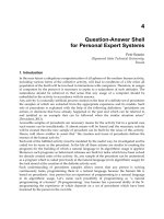
added directly. For instance, if there are two identical sources, their sound
levels are added together by adding 3 Db to the sound from the single
source. If we have ten such sources, the number of decibels to be added is
10, and the other intermediate values follow the curve in the Figure 7.9.
If the sources being added are not identical, the decibels to be added (to
the noisier source) depend on how different the two sources are, ranging
from 3 Db if both sources are equal, to 1 Db if the second source is 6 Db
below the first, to virtually zero if the second source is about 20 Db
0
2
4
6
8
10
12
0.0 2.0 4.0 6.0 8.0 10.0 12.0
decibels added
number of identical sources
Series1
Figure 7.9 Accumulation of noise with multiple sources.
© 2004 Agustin Rodriguez-Bachiller with John Glasson
Hard-modelled impacts 209
below.
29

This complication also arises when adding sound levels over time,
for instance to calculate average levels over a certain period which, as we
shall see, is central to the assessment of noise impacts.
Another mathematical complication is related to the frequency at which
a sound is emitted. The perception of sound varies with its frequency and,
for most part of the hearing spectrum (up to 4000 Hz), a sound at a certain
number of decibels and a given frequency will be perceived as being as loud
(in “fons”)
30
as another sound at a lower frequency and a higher number of
decibels. This means that often, in order to reduce different sounds to
comparable scales of “perceived” loudness (and in order to compare them
to the relevant standards), all the sounds emitted at a variety of frequencies
must be converted into their equivalent at a standard frequency (usually
1000 Hz). The conversion is normally done by adding (or subtracting) to
the sound level at each frequency a number of decibels, normally calculated
from the so-called “A” curve, the iso-loudness curve corresponding to 40
fons. Sometimes, logarithmic aggregations are combined with this conversion
process, for instance when we need to calculate the sound level from a
complex source emitting at several frequencies: in order to calculate the
“perceived” overall level, we must first convert the sound levels at each
frequency to their 1000 Hz-equivalent, and then all the equivalent levels
can be added logarithmically.
These apparent complications in the calculations are really used to adapt
a complex theoretical framework necessary to understand sound propagation
and perception so that it can be used in practical situations and with a realistic
amount of information. As in air pollution, the modelling of noise impacts
is a compromise between scientific soundness and practicability, and an
important part of the expertise in this field is to be aware of how such com-
promise and simplification may affect the results or their interpretation.

As in air pollution, noise-impact assessment can be applied at various
stages in the life of the project and/or of the impact study although in its
own peculiar way. Also, various types of impacts (noise, vibration, and
“re-radiated” noise transmitted through solid materials) are included under
the general heading of “noise”, and they present quite different challenges
adopt a similar framework to that used for air pollution, adapted to these
variations.
31

29 For graphs showing this relationship as a continuous curve, see any technical references
like Mestre and Wooten (1980) or Therivel and Breslin (2001).
30 The fon-level of a sound is equal to its decibels at 1000Hz.
31 The knowledge acquisition for this part was greatly helped by conversations with Stuart
Dryden, of Environmental Resources Management Ltd (Oxford branch), and Joanna C.
Thompson helped with the compilation and structuring of the material. However, only the
author should be held responsible for any inaccuracies or misrepresentations of his views.
© 2004 Agustin Rodriguez-Bachiller with John Glasson
and require very different approaches (Figure 7.10). The following sections
210 Building expert systems for IA
7.3.1 Project design
As with air pollution, noise experts can advise project designers on the
basis of their “anticipated” impact calculations resulting from one design
or another, not necessarily based on actual calculations or “runs” of a
model, but on their expert knowledge of the mathematics involved and on
their experience. Because of the nature of noise – an oscillatory phenomenon
travelling in straight line in all directions – the main considerations in terms
of noise impacts tend to be associated with the relationship and proximity
between noise sources and receptors deemed to be potentially sensitive (e.g.
housing, schools, hospitals, libraries). In particular, advice at the design
stage involves:

•
First, the broad identification of potentially sensitive receptors nearby
(GIS can help with this)
32
anticipating a more systematic search to be
carried out for the baseline and impact assessments.
•
Second, the advice usually refers to the possible repositioning of noise
sources and/or with the interposition of barriers between them and the
potential receptors (very much like “anticipated” mitigation measures).
Repositioning of noise sources can be the basis for advice on possible
alternative locations for the project further away from sensitive receptors,
or it can be the basis for changes of position within the project: to a different
32 For example, GIS functionality can be used to identify the nearest building of certain type
of use.
Figure 7.10 Types of noise impacts.
© 2004 Agustin Rodriguez-Bachiller with John Glasson
Hard-modelled impacts 211
side of the site, from outside to inside a building, to another side of a building.
Encasing a source inside a building can be similar to erecting a barrier
between the source and the receptors, but other types of barriers, such as
solid, vegetation or sinking the source into a ditch, can also be used
(Figure 7.11).
Some of these anticipatory modifications are no different from possible
mitigation measures, only here they are considered before the details of the
project have been finalised. In practice, one of the problems of “anticipating”
noise impacts at the project-design stage is that noise experts are often
consulted at the wrong time (Dryden, 1994). It can be too early in the
design process, before the developers know the details and location of all
the ancillary equipment that is going to be used, before they know the location

and nature of all the noise sources. Or it can be at the other extreme, after
everything has been decided and the design finished, when changing any-
thing can have many knock-on effects requiring further changes. The ideal
situation would be if developers consulted the noise experts while the
design is taking shape.
7.3.2 Noise baseline assessment
As in air pollution, the determination of noise levels in the area where the
new project is likely to have an impact is central to the impact assessment,
and the baseline situation must be measured in a way that can be compared
with the relevant standards for the particular project. Again, this relates to
what is being measured – noise in this case (no baseline study is made for
vibration or re-radiated noise) – and also to its type of manifestation,
Figure 7.11 Project information for noise-impact assessment.
© 2004 Agustin Rodriguez-Bachiller with John Glasson
212 Building expert systems for IA
particularly its concentration over time: averages, peak values, etc. But the
approach differs in other respects, derived from two intrinsic differences:
•
Air-dispersion modelling is highly inaccurate – making references to
specific locations largely irrelevant – but noise modelling is not, and
this gives the noise baseline assessment a totally different “shape”: The
first stage in the baseline assessment is the identification of potentially
sensitive receptors, their nature, location and distance from the noise
sources, and it is at those receptors that the baseline situation will be
measured.
•
Pollutant concentrations are difficult and expensive to measure for an
individual case and we tend to rely upon existing monitoring pro-
grammes, of which there are sufficient variety. But noise measurement
is relatively simple and inexpensive, with portable equipment quite

easy to operate, which makes it possible to identify specific locations
considered relevant to our study (the sensitive receptors) and, in the
second stage of the baseline assessment, to carry out the monitoring
directly.
The search for receptors starts around the project in ever-widening circles,
and keeps increasing to about 500 m (only exceptionally beyond 1 km) until
receptors are found in a sufficiently wide range of directions, but this may
be related to the type of project. For instance, in projects involving new
roads, a crucial distance for receptors is 300 m – properties within this
distance can be entitled to compensation
33
– or, for projects expected to
run also during the night (like a railway line, or a power station), the search
distance can be much greater. The search for receptors can go further than
any noise is likely to reach, but as a general rule, locating the receptors,
rather than specifying the distance, is the issue (Dryden, 1994). What is
crucial is to identify the front line of receptors. How deep beyond this front
line the baseline assessment needs to go is largely determined by the expec-
tation of success or failure in the mind of the expert, largely based on
experience, of the noise-impact measurements. If the project “looks like”
not violating the standards at the front-line of receptors, the search does
not need to go further, as noise decreases with distance. Also, if infringe-
ments of the noise standards are clearly expected, again the measurements
do not have to extend further. Only when the noise impact is expected to
be marginal – violating some standards but not by much – that the identifi-
cation of receptors needs to extend over a fringe of a certain depth, deter-
mined by the additional distance expected to make the impacts fall below
acceptable levels. That distance will depend upon the source, the topography,
33 For example, in the UK, properties within 300 m of new roads are eligible for noise
insulation paid for by the developer responsible, and GIS “buffering”can be used to

identify them.
© 2004 Agustin Rodriguez-Bachiller with John Glasson
Hard-modelled impacts 213
and a number of other factors such as the anticipated opportunities for
mitigation. How easy and practical a reduction of noise impacts would be
by mitigation are at the forefront of the expert’s considerations even at this
early stage.
Usually the search – or at least the “planning” of the search – is based on
a map of the area, and GIS could be used to do it automatically. A field
visit is useful to check local features, variations in the topography, or the
potential receptors themselves, and such a visit may change our priorities
over which receptors to study. For example, what is thought to be a
building, a potential candidate for “receptor”, from the map may be just a
half-demolished shed.
Sometimes the sensitivity of the receptors is compounded by the state
of local opinion, in which case the Local Authority is an important
source of information as to local sensitivity and even the location of any
foci of concern. It might therefore be an advantage to carry out measure-
ments close to the properties where the occupiers are known to be con-
cerned, in order to clarify the situation. On the other hand, if the
situation has reached the point of potential conflict, baseline recordings
may be limited to public rights of way, or to land owed by the same
developer behind the project. Sometimes developers start tentative
enquiries about possible impacts at an early stage in the design of the
project, before the details are known. This can have the effect of sensitising
public opinion against the project and, in such situations, recording
baseline noise at some locations over extended periods of time may
encounter local opposition, and a modification of the schedule of recordings
may be needed.
In terms of the types of measurements to use for baseline assessment,

particularly their time dimension, the same general criteria apply as in air
pollution, including an idea of the general average levels of what is being
measured (noise), plus some idea of the peaks to be expected over time. In
sound-level measurement, there are some well-established types of indicators
ranging from those which measure “averages” to those which measure
“peaks”:
•
The “equivalent continuous noise level” (L
eq
) is the level of steady noise
which would have produced over a period of time the same energy
as the various noise levels present over that same period (combined
logarithmically using the A-weighting curve).
•
The “background noise” is usually measured by the noise level
exceeded over most (90 per cent) of a period of time (L
90
), undertaken
by recording the duration of each noise level and defining the cut-off
level of the worst 90 per cent by simple statistical analysis.
•
Other similar indices like L
50
(using only the worst 50 per cent of the
period, somewhere in between measuring averages or peaks) are used
much less frequently.
© 2004 Agustin Rodriguez-Bachiller with John Glasson