Expert Systems and Geographical Information Systems for Impact Assessment - Chapter 9 pps
Bạn đang xem bản rút gọn của tài liệu. Xem và tải ngay bản đầy đủ của tài liệu tại đây (1.2 MB, 45 trang )
9 Socio-economic and traffic
impacts
9.1 INTRODUCTION
With the exception of ecological impacts, most impacts are assessed by the
repercussions they have on humans (noise, air pollution, landscape, etc.)
and to that extent they all could be considered social in nature. However,
impacts usually referred to as “socio-economic” have the characteristic that
they are transmitted through the workings of society itself, its economy and
the behaviour of its population as a result of the project. In this respect,
traffic impacts can also be considered under the same heading, as they also
result directly from social behaviour – with vehicles as “instruments”. This
view of socio-economic impacts suggests the need to consider how society
works in order to assess any impacts on it, and that can face us with
a problem similar to what we found when dealing with ecology, i.e. the
extreme complexity of the science that studies the field, in this case, social
behaviour. It can be argued (Vanclay, 1999) that social impacts have
always been the central concern of the social sciences, and that to analyse
these impacts we have to use the rigour of such sciences. In this sense, the
usual approach to the study of these impacts can be said to only “scratch
the surface” of social impacts, concentrating on relatively superficial indicators
of impact but without getting into their deeper social repercussions in terms
of social change, the true measure of social impact. On the other hand, in
practical terms it might prove difficult to engage in deep social research
involving wide-ranging surveys for every project requiring this type of
impact assessment. This is one of the dilemmas of socio-economic impact
assessment – and one that impact studies address in varying degrees – especially
since this area of impact assessment is relatively new and still has to become
fully established as part of the standard collection of impacts to consider.
9.2 SOCIO-ECONOMIC IMPACTS
These types of impacts are relative newcomers to impact assessment, as the
initial emphasis of this growing area of interest and legislation was placed
© 2004 Agustin Rodriguez-Bachiller with John Glasson
Socio-economic and traffic impacts 273
more on “environmental” impacts, probably on the assumption that the
socio-economic side was already being covered by the town planning
system (Glasson, 2001). Only in the 1990s did socio-economic impact studies
become a standard component – albeit sometimes rather “thin” (Glasson,
1994)
37
– of a growing number of environmental statements, following the
good-practice literature which has accompanied this “coming of age” (Petts
and Eduljee, 1994b; Glasson, 1995, 2001; Chadwick, 1995, 2001; Vanclay,
1999; Chadwick, 2001 also contains a very good bibliographical compila-
tion). There has been some debate about the nature of, and what to include
in, socio-economic impacts. Our definition of these “people impacts”
includes direct economic impacts, which normally lead to indirect wider
economic/expenditure impacts, demographic, housing, other social services
(such as education, health, police) and socio-cultural impacts (including
lifestyle, community integration, cohesion and alienation). The general
logic advocated for these studies is similar to that of other impacts
(Figure 9.1).
Although economic and social impacts can be studied separately – partly
because economic impacts tend to be positive while social impacts tend to
be negative – the logic they follow is similar, and usually starts from a common
base, and it is only after “scoping” the impacts that the two lines of enquiry
separate.
37 The face-to-face part of the knowledge elicitation for this area of impact was approached
in a way similar to the other areas of impact, i.e. by holding structured conversations
between Agustin Rodriguez-Bachiller and an expert in the field, even if in this case the
expert (John Glasson, of the Impact Assessment Unit in the school of planning, Oxford
Brookes University) was part of the authorship of this book, and references to those
conversations will be made in the usual manner. Duma Langdon helped with the compilation
and structuring of the material for this part.
Figure 9.1
The logic of socio-economic impact assessment.
© 2004 Agustin Rodriguez-Bachiller with John Glasson
274 Building expert systems for IA
9.2.1 Understanding the project
In socio-economic terms, what matters about the project is its capital investment
and its human-resources (labour and users/customers) plans for the con-
struction and operation stages, the study of the latter often extending up to
2–3 years into full operation. This involves first of all the detailed quantifi-
cation of the socio-economic components of the project, but also it
concerns more qualitative social/employment policies associated with it
(Figure 9.2). Starting with the quantitative information, concerning the
expenditure in physical factors first, we need to know the magnitude and
nature of the project:
1For the construction stage, the investment over time in:
•
infrastructure,
•
equipment,
•
buildings,
•
non-labour services.
Figure 9.2 Information about the project for socio-economic impact assessment.
© 2004 Agustin Rodriguez-Bachiller with John Glasson
Socio-economic and traffic impacts 275
2For the operation stage, the expenditure over time on:
•
goods,
•
raw materials,
•
non-labour services,
•
maintenance.
On the human resources side, we need to know:
1The “labour curves” over time for construction and operation (see an
•
number of workers,
•
occupational categories/skills.
Differences in the labour force between construction and operation
can be important, as some infrastructure/utilities projects (like power
stations, roads) involve much more labour during construction than
operation, while manufacturing and especially service projects (business
parks, new settlements) tend to the opposite. On the other hand, when
the latter happens it tends to be because of a high number of visitors/
users, and not because of a high number of workers operating the
project, as most types of projects tend to be more and more capital-
intensive.
2 Visiting users/customers over time (only for the operation stage):
•
numbers,
•
socio-economic profile.
In the construction stage it is unlikely that there will be significant numbers
of visitors, users or customers, and in some types of projects (like energy
projects) this will also be the case for the operation stage. Other projects
(like leisure facilities, retail parks, new settlements) depend on large
numbers of visitors/users, whose impacts must be considered.
On the qualitative side, it is crucial to identify the developer’s policies
concerning labour practices on the one hand, and the expected level of local
sharing in all the activities, on the other. On the working practices, it is
important to know:
1 wage levels;
2 shifts to be used (e.g. two or three);
3 accommodation policies (like provision of an on-site hostel);
4 transportation policies:
•
bussing workers (especially for the construction stage),
•
providing travel allowances up to a certain distance.
© 2004 Agustin Rodriguez-Bachiller with John Glasson
example in Glasson, 2001):
276 Building expert systems for IA
Also, it is most important to find out if the developer has any specific
policies about the expected local share of each part of the project:
1 Expected proportion of local/non-local labour, usually decreasing as
the skill level increases; Glasson (2001) gives a typical profile of the
proportions of local labour expected in major projects:
•
site-services, security and clerical: 90 per cent,
•
civil engineering operatives: 55 per cent,
•
mechanical and electrical operatives: 40 per cent,
•
professional, supervisory and managerial: 15 per cent.
Sometimes developers are less inclined to employ local labour when the
area has a reputation for labour problems.
2 Training policies: including training in the employment package can be
useful to overcome any prejudice against taking on local unemployed
people. As a general rule, the higher the occupational category of the
staff the longer will be the training needed and the less likely workers
are to come from the locality.
3 Policy on local suppliers and putting contracts out to tender: in the
construction stage, during normal operation.
4 Purchasing agreements that the firm running the project (often a
national firm) may have with non-local firms.
As a result of some of these policies, a profile will emerge of the proportion
of workers at different occupational levels likely to be in different family/
housing situations (during construction and operation):
•
workers in-migrating to the area with their families: in the construction
stage – if it lasts for several years – it will be of the order of 10 per cent
or 20 per cent of the external workforce, during operation it is likely to
be the vast majority (90 per cent) of the in-migrating workforce;
•
workers in-migrating to the area but without their families;
•
long-distance commuters;
•
local workers.
Although all this information about the project is necessary to carry out
a detailed impact study, developers cannot always provide it. Decisions on
some aspects of the project (like staffing) may be at an early stage and we
can either use aggregate figures for labour or investment (and carry out the
analysis at an aggregate level) or we can use other similar projects as
sources of comparative information to “flesh out” the project, when estimating
the likely composition of the labour force, or the likely proportions to be
in-migrants, commuters, or locals.
© 2004 Agustin Rodriguez-Bachiller with John Glasson
Socio-economic and traffic impacts 277
9.2.2 Understanding the baseline
The next step is to understand the host society which the project is likely to
impact. As with the project, the study of the socio-economic baseline
involves on the one hand finding out about the social situation from data
and, on the other, finding out what the social attitudes and sensitivities are,
which give social meaning to the data (Figure 9.3). Studying the facts alone
may allow us to calculate the quantitative value of some of the impacts, but
it will reduce the study of their significance to the kind of technocratic
study of indicators (the “checklist approach”) which Vanclay (1999) critically
refers to, and only the study of the local culture will give us sufficient
information to assess the significance of those impacts.
Figure 9.3 Baseline study for socio-economic impact assessment.
© 2004 Agustin Rodriguez-Bachiller with John Glasson
278 Building expert systems for IA
The first step is to define the area(s) of study, trying to match as much as
possible the “areas of influence” of the project. The most important of
these areas of influence is the commuting area for the project workers:
•
For the construction stage, it can be substantial and, for some workers,
up to the 90-min isochrone or beyond, as short-term construction
workers are prepared to travel longer distances.
•
For the operation stage, the catchment distance is usually considered
closer, with workers usually living near to a project at which they may
work for many years.
When dealing with projects that involve visiting users/customers, a different
type of travel area can come into the picture, the market area of the project.
When such catchment area is known – maybe as part of the “business
plan” of the developer – it can be used to identify the socio-economic
profile of those users/customers. Sometimes the developer does not know
the customers’ catchment area – maybe the business plan has not been
drawn in those terms – but in that case the developer will have a good idea
of who the customers will be (which is really the information we are after),
and we can get that information directly, without having to extract it from
published information about the area they are likely to come from.
With these general criteria in mind, the question is to define area(s) of
study as close to these catchment areas as possible, whilst at the same time
trying to maximise the amount of published information available for those
areas; the final decision is usually a compromise between the two criteria. It
is common for the study to use several sets of study areas – each providing
their own set of data – as long as they overlap sufficiently with the “core”
area of influence, and as long as they do not differ too much from each
other. The final data-collection area may end up being a superimposition of:
•
Local authorities, well documented in the Census: in the UK, a County
can be a good starting point, sometimes complemented with additional
Districts (and even Wards) around it.
•
The Department of Employment’s “Travel to Work Areas”, which are
quite large and can be adequate for the construction stage, but they
tend to be excessive for the operation stage.
•
Health Authorities are too large, but they can provide good data on the
health-care situation.
•
Similarly, Police Authorities are also too large, but they provide good
data on the crime-prevention situation.
For the respective areas of influence – however defined – the information
to be collected helps to put together a picture of the capacity of the area (in
economic terms and in social terms) and the existence of any surplus or
deficit in any of these aspects, which will help determine the extent of any
© 2004 Agustin Rodriguez-Bachiller with John Glasson
Socio-economic and traffic impacts 279
impacts. But we also need to find out the perceptions and attitudes of the
various sectors of the local population about what are the problems (if any)
in the area, as it is these perceptions that will ultimately shape the “meaning”
of the new project for the local population and the significance of its
impacts. With this double objective in mind, the “information sweep” should
be carried out at several levels through:
1 Desk-based data collection from published statistics and local studies if
they exist.
2 Assessment of social perceptions and feelings in the area:
•
establishing liaison groups between the study team, the developer
and the community;
•
browsing through the local press;
•
talking to employment and planning officers in the local author-
ity to check if something is “going on” such as problems develop-
ing, other competing projects coming to the area, or local
anxieties;
•
talks with the Department of Employment’s manpower sections
about local labour markets, and their policies and opinions about
incoming change;
•
interviews with key-individuals in the community;
•
investigating general public opinion directly, either informally,
in casual conversation with locals while doing other parts of the
field work, or formally, by more organised public information-
gathering: (i) by systematic surveys on specific issues identified
informally; (ii) in public meetings organised to increase public
awareness of and participation in the impact assessment exer-
cise; such meetings normally refer to all aspects of the project
(and not just to its socio-economic side) and can represent one of
the few points in the impact assessment process where all areas
of impact assessment come together. This type of systematic
investigation of public opinion presents the usual problems
discussed before about public participation: although impact
assessment experts invariably think it a good idea, developers
tend to be reticent about it, as it can raise awareness about the
proposed development and generate a reaction against it from
quite early in the process. This is a typical example of what
Vanclay (1999) refers to when saying that one of the problems
of social research is that the investigation itself can change the
social reality it is investigating.
The “information sweep” can be summarised in the following checklist
© 2004 Agustin Rodriguez-Bachiller with John Glasson
(for a fuller discussion see Glasson, 2001 and Chadwick, 2001):
280 Building expert systems for IA
For the economic side of the study:
1 The situation of those in employment in local firms:
•
age,
•
gender,
•
economic sector,
•
occupational category.
The best source for this type of data in the UK is the National Online
Manpower Information System (NOMIS), which can be accessed by
subscription.
2The unemployment situation:
•
numbers unemployed,
•
how long unemployed,
•
occupational category.
The best source for this information in the UK is the Department of
Employment Data Sources (e.g. Labour Market Trends) that update
and publish unemployment, vacancy and redundancy data on a
monthly basis, and with a regional disaggregation.
For the social side of the study:
1 Population
(a) latest figures by age groups from the Census (sometimes going
down to Ward level with the Small Area Statistics)
(b) population trends:
(i) from the mid-year estimates;
(ii) population projections for Regions and Counties produced by
the Office of National Statistics;
(iii) Planning Local Authorities usually have working figures about
population trends at County and District levels as part of the
Structure and Local planning activity.
2 Housing
(a) the latest stock (from the Census or from surveys by the local
authority): deficits, surpluses (e.g. under-occupation), vacancy rates,
second homes;
(b) housing prices/rents (from local estate agents and newspapers, also
from some local Building Societies);
© 2004 Agustin Rodriguez-Bachiller with John Glasson
Socio-economic and traffic impacts 281
(c) housing construction/renovation trends (from “Local Housing
Statistics” in England and Wales and “Housing Trends” in Scotland);
(d) availability of temporary accommodation (normally for tourism)
as a possible accommodation alternative, especially for construction
workers: Bed and Breakfast, guest houses, caravan sites
(in the UK, the Regional Tourist Boards have good information
about local capacity and occupancy rates; local Tourist Informa-
tion Centres can often provide more “on the ground” information);
(e) with respect to trends in the supply of tourist accommodation,
local authorities will have information from the inflow of planning
applications.
3 Education
In the UK, Local Education Authorities have good information on
education, which can be complemented with data from the Department
of Education and Employment:
(a) current supply (schools and Colleges of Further Education): capacity,
numbers of pupils, pupil/teacher ratios;
(b) trends and planned changes: trends in local demand can be calcu-
lated by “rolling on” the data collected about people of school age,
although with the increased freedom of choice of school, the level
of use of schools is influenced not only by local demographics, but
also by how each school compares with others.
4 Health
In the UK, the following kind of information can be provided by the
Family Health Service Authorities and by the Regional Health Authorities:
(a) General Practitioners in the area;
(b) size of doctors’ lists;
(c) turnover of doctors;
(d) spare capacity in local hospitals (if any).
5 Social services
From the Department of Health and Social Security, information can
be gained on:
(a) homes for the elderly: places, spare capacity;
(b) children’s homes: places, spare capacity.
© 2004 Agustin Rodriguez-Bachiller with John Glasson
282 Building expert systems for IA
6 Police and emergency services
From the Police Authorities, data can be obtained on crime/arrests and on
general feelings about the crime-prevention situation. This can be extended
to other emergency services if it is perceived that there are problems of
capacity or dissatisfaction in the area concerning those services.
7 Social facilities
As with other services, what interests us here is the existing capacity and
whether it is considered sufficient, if there is spare capacity, if any of these
facilities (or the lack of facilities) create problems for the community or
for the authorities, such as the police: leisure, sports, pubs, clubs.
The socio-economic field is one of the very few areas of impact assessment
where trends in the baseline (without the project) are central to the assessment.
Population projections (10–15 years ahead) for the local area are crucial,
and from them other projections are made of demand for housing, schooling,
health care and other services. Geographic information systems can be
used as a storage and “synthesizer” of large amount of information (from
the Census and many other sources) and, to that extent, an existing GIS
with all or part of the information needed for the baseline could be used at
this stage as an important source. In this context, GIS would not really be
used in its analytical capabilities, but only as a database with the ability to
display maps of the information, with the advantages this can add to the
understanding of the area.
The ultimate objective of the information sweep is twofold: (i) to determine
the capacity (present and future) of the system for extra jobs and extra
demand for services; and (ii) to understand how the local population feel
about the situation and the incoming change. This should give an idea of
the aspects of society where the new project is likely to produce its impacts,
which will need to be investigated further.
9.2.3 Economic impact prediction
It is at this point that the economic and social lines of enquiry part com-
pany, not because their objectives differ but because the approaches they
use diverge. Economic impacts could be interpreted in a wider sense, to
mean all the economic effects of the project and the transformation –
quantitative and qualitative – of the local economy that could result.
In practice, however, the study of economic impacts focuses on the likely
overall quantitative growth that a project can generate, and this growth is
usually studied focussing on two areas: (i) changes in Local Authority
finances, and (ii) growth in the local economy. First, the financial situ-
ation of the Local Authorities affected are likely to change in various
ways (Chadwick, 2001):
© 2004 Agustin Rodriguez-Bachiller with John Glasson
Socio-economic and traffic impacts 283
1On the income side:
(a) there will be increases in council tax, as new people buy property
in the area;
(b) population increases will mean changes in the Local Authorities’
position in the calculation of the “Standard Spending Assessment”
contribution by central government (which are proportional to the
resident population), although short-term temporary workers will
not make a difference;
(c) similarly, there should be an improvement coming from non-
domestic rates, which are paid to a central pool and then re-allocated
to Local Authorities by population levels.
(information on this can be found in “Finance and General Ratings
Statistics” [“Rating Review” for Scotland] from the Chartered
Institute of Public Finance and Accountancy Statistical Information
Service)
2On the expenditure side, the effects of growth can be more difficult to
calculate, as the published figures on the various costs allow the calcu-
lation of average costs, which in reality “hide” two types of costs: fixed
costs which do not change with growth and variable costs (per head)
that do, and the growth in expenditure would only affect the latter.
With respect to the growth of the local economy, it can be quantified in
terms of employment or income but the basic reasoning is the same: an
injection of new demand for workers and/or goods will make the local
economy grow, and the question is to forecast by how much. It is known
from economic theory that the economic effect of an expenditure in an
economic system is greater than the original amount because of the
“cascade effects” it generates, as if the original injection had been “multiplied”
by a factor greater than one. Hence, the calculation of this type of economic
magnitude of the economic injection, the “multiplicand”, and the greater-
than-one multiplying factor, the “multiplier”.
9.2.3.1 The multiplicand
A development project usually generates several injections into the
economy – some are one-off and some are permanent during the life of
the project. For the purposes of multiplier analysis, these injections can
be grouped under two main headings: investment and jobs, both during
construction and operation. If the information available about the
project is limited to overall figures and we are carrying out the study at
an aggregate level, these two project injections will constitute our main
multiplicands.
© 2004 Agustin Rodriguez-Bachiller with John Glasson
effect focuses on calculating the two elements involved (Figure 9.4): the
284 Building expert systems for IA
If a more disaggregated approach is attempted, these injections are
broken down into a more detailed list of multiplicands:
1During the construction stage, assumed to happen once (if there are
expansions/modifications to the project later, for the purposes of
impact assessment they are considered in most cases as new projects
and their impacts need to be assessed afresh):
(a) the initial investment involved in the creation of the project (infra-
structure, buildings, equipment);
Figure 9.4 The multiplier.
© 2004 Agustin Rodriguez-Bachiller with John Glasson
Socio-economic and traffic impacts 285
(b) labour (and their wages) to work in the construction of the project:
(i) coming from outside the area: single temporary in-migrants,
temporary in-migrants with their families, temporary long-
range commuters;
(ii) local labour.
2During the operation of the project (these multiplicands apply during
the life of the project):
(a) regular demand for inputs (goods, raw materials, services, rented
floorspace);
(b) stable labour (and wages) to work in the project:
(i) coming from outside the area: single permanent in-migrants,
permanent in-migrants with their families, permanent long-
range commuters;
(ii) local labour;
(c) expected users/visitors and their expenditure in the local area (not
in the project, e.g. entrance fees).
Not all these categories will be present in all projects, and some will be
negligible and not worth calculating (like the number of permanent long-range
commuters for the life of the project), although some of these categories
“evolve” into others: for instance, it is common for long-range commuters
to become in-migrants, or for single in-migrants to bring their families later
if the labour situation stabilises.
If we are following a disaggregated approach to our multiplier analysis,
it is useful to consider the different multiplicands separately, not because
they are conceptually different – we can add apples and pears if we are only
interested in their cost – but because they work their way into the system
differently. In particular, these multiplicands do not apply “in full” to
the local economy because they suffer “leakages” to the outside. Typical
multiplicand leakages are:
1 Leakages from the initial investment (the construction stage) which can be:
(a) the equipment – and its installation – which the firm undertaking
the project brings with it, maybe because it involves specialised
technology not available locally, like a nuclear reactor or a waste
incinerator;
(b) goods or services likely to be imported during construction, maybe
due to prior arrangements with other outside firms.
© 2004 Agustin Rodriguez-Bachiller with John Glasson
286 Building expert systems for IA
2 Similar leakages can happen during operation:
(a) raw materials, goods and services for the running of the project
imported from outside the area, sometimes due to prior purchasing
agreements with other firms;
(b) property rents going to landlord’s resident outside the area;
(c) profits going to shareholder’s resident outside the area.
From the earlier investigation of the project, where we quantified all the
investments and jobs involved (if the information was available), these
leakages must be deducted and the residual amounts spent locally can be
calculated, for use in the next stage in combination with the economic
multiplier.
9.2.3.2 The multiplier
Although there are various types of multipliers,
38
it is the Keynesian version
that is normally used for this type of study. We can expect these multipliers
to be greater than one. In fact, the so-called “income multiplier” would be
infinite were it not for multiplier leakages (in addition to the multiplicand
leakages discussed before). Multipliers are usually expressed by a formula
of the type 1/(1
−ƒ
leakages
) where the function
ƒ
depends on the particular
way in which the leakages are calculated. In the UK, the standard approach
derives from early discussions of “regional” multipliers (Brown, 1967;
Steele, 1969), and starts from an adaptation of the classic Keynesian
way of expressing a change Y in the Gross Domestic Product of an
economic system (national, regional or local) at factor costs in terms of its
components:
Y
=
J
−
T
d
−
U
+
C
−
M
−
T
i
J expenditure on value added in the area, this is the “autonomous” part
of the equation, usually taken to mean the “injection” of resources
from outside the system which, in our context, can be used also to
represent public or private investment on development projects
2001) differ in the level of disaggregation they use to look at the economy and its inter-
actions: the Input–Output approach breaks down the economy into (many) economic
branches, the Economic Base approach breaks down the economy into basic and non-basic
activities, and the Keynesian approach considers the economy as a whole. Partly because
of this, the first two become quite difficult to use at local level: with respect to the Input–
Output approach, it is virtually impossible to find a reliable local I–O table; with respect to
the Economic Base approach, there are conceptual difficulties in defining what is basic and
non-basic at the local level.
© 2004 Agustin Rodriguez-Bachiller with John Glasson
38 The three most commonly known approaches to the definition of multipliers (see Glasson,
Socio-economic and traffic impacts 287
T
d
direct taxes (like Income Tax), a leakage which can be expressed as
t
d
×
Y (where t
d
is the marginal propensity to pay taxes with rising Y)
U change (decline) in transfer payments (unemployment benefits for
example) from Government with rising income and employment, a
leakage which can be expressed as u
×
Y (where u is the propensity to
lose transfer payments with rising Y)
C change in consumer expenditure at market prices, which can be
expressed as a function of the income left after deducting the previous
leakages (direct taxes and loss of transfer payments): c
×
(Y
−
T
d
−
U)
where c is the marginal propensity to consume part of the disposable
income left
M imports for consumption, a leakage that can be expressed as a func-
tion of consumption m
×
C (where m is the marginal propensity to
import with rising consumption) which, substituting the expanded
expression for C, becomes: m
×
c
×
(Y
−
T
d
−
U)
T
i
indirect taxes (like Value-Added Tax), another leakage, which can be
expressed as a function of “local” consumption (after discounting the
imports) t
i
×
(C
−
M) where t
i
is the propensity to pay indirect taxes
with rising consumption which, substituting the expanded expres-
sions for consumption and imports, becomes: t
i
×
(Y
−
T
d
−
U)
×
(1
−
m).
Substituting T
d
and U by their expressions (t
d
Y and uY) and substituting all
these expressions into the master equation for Y, we get:
Y
=
J
+
Y
×
c
×
(1
−
t
d
−
u)
×
(1
−
m)
×
(1
−
t
i
)
It has also become standard practice (Steele, 1969) to assume consumption
and saving as complementary, and C can be substituted by Y
−
T
d
−
U
−
S in
the master equation, where S (savings) is another leakage which can be
represented as s
×
(Y
−
T
d
−
U) where s is the marginal propensity to save,
and it is assumed that c
=
1
−
s. Substituting in the last equation and simpli-
fying, we derive the standard formula for the multiplier (Glasson, 2001):
We can see that the increase in value-added Y would be equal to the
“autonomous investment” J multiplied by a factor greater than one (as the
denominator is less than one). The succession of expressions in brackets
expresses how leakages “accumulate”, each one applying to what is left
after the others. The main problem with calculating these leakages is the
difficulty of knowing marginal propensities – representing the proportions
of the next income increase to be used in various ways – and the usual
compromise is to use average propensities instead, which represent the
YJ
1
11s–
()
– 1 t
d
– u–
()×
1 m–
()×
1 t
i
–
()×
×
=
© 2004 Agustin Rodriguez-Bachiller with John Glasson
288 Building expert systems for IA
proportions of the whole income. Unless fresh survey data is available to
estimate the likely proportions of extra income to be used in different ways,
published information usually shows overall figures, and proportions
calculated from them will only represent average behaviour and not
marginal behaviour. This is not a major problem in some cases (unemployment
benefits or VAT, for instance) when the proportion lost will be the same
independent of the level, but in most other cases (direct taxation, savings,
imports) it is well known that the proportions tend to increase with
income.
Having calculated the multiplicands – coarse or disaggregated – derived
from the project (see previous section), what we have to do now is to:
•
calculate the multipliers which apply to each multiplicand;
•
multiply each multiplier by its multiplicand;
•
add up all the multiplications, and this sum will be the total economic
impact.
Sometimes the disaggregation of the multiplicand can introduce compli-
cations that require modifications of the way we calculate the multiplier.
For instance, Brownrigg (1971) modified the standard calculation of the
multiplier to account for in-migration of some of the labour force, breaking
down the calculation of the multiplier into two stages:
•
First, in-migrant workers inject some of their demand for goods and
services into the local economy, with their own propensities to leak
(ignoring the loss of transfer benefits, and using average propensities,
as all their income is used for the calculation) and their first-round multiplier
(M
1
) can be calculated.
•
Second, this “multiplied” injection into the local economy generates its
own subsequent-rounds multiplier (M
2
) for the whole local population,
calculated using the normal procedures and propensities (marginal if
possible).
•
Finally, the overall multiplier for this particular labour group can be
calculated as 1
+
M
2
×
(M
1
−
1).
Local area multipliers normally vary between 1.1 and 1.4 (Glasson,
2001) meaning that for each pound brought directly by the project, an
extra 10–40 p is generated indirectly. The range of values is relatively
narrow, and if we are carrying out an aggregate multiplier analysis (maybe
because the budget for the project is not high) it is possible just to
“borrow” these values and assume that they will apply to our project,
expressed as a range (1.1–1.4) or as an average (1.25).
Even if we are carrying out a disaggregated study of the various multipli-
cands, and given the difficulties of calculating propensities, we can:
© 2004 Agustin Rodriguez-Bachiller with John Glasson
Socio-economic and traffic impacts 289
1 Borrow the multiplier values for some of the multplicands from other
studies of similar projects; for example, power-station impact studies
have produced consistent multiplier values for typical labour groups
(Glasson, 2001):
•
for in-migrant workers without families 1.05–1.11 (between 5 p
and 11 p extra);
•
for in-migrant workers with families 1.3–1.5 (between 30 p and
50 p extra).
2 Or we can calculate the propensities (to leak) and the multipliers for
the disaggregated multiplicands from scratch.
Calculating the various propensities associated with each type of multi-
plicand we can sometimes use some simplifications:
•
Some propensities can be ignored (assumed zero) with some multipli-
cands: for example, when calculating the multiplier for outside labour,
we can ignore changes in transfer payments like unemployment benefits,
as incoming labour may prevent a fall in local unemployment.
•
Some propensities will be common to all multiplicands (like Value
Added Tax).
•
Some propensities will be common to several multiplicands (like the
propensity to save or to pay taxes) likely to be similar for all labour of
the same occupational standard irrespective of whether they are local
or not.
39
The single most important propensity, which is likely to show the greatest
range of variation and the greatest influence on the final value of the multiplier,
is the propensity to import. It is also one of the most difficult to calculate for
sub-national economic systems, given the difficulty to find published data on
imports–exports between regions, let alone smaller areas like the ones normally
used in impact assessment. We can try to get around this problem by:
•
“Borrowing” import propensities from studies which have used a
similar breakdown of multiplicands; for instance Glasson et al. (1988)
found when studying power stations in fairly remote locations that the
propensity to import for in-migrant workers with their families could
be as high as 0.6–0.7 (60–70 p).
•
“Approximating” the quantification of imports–exports with indicators,
a typical example of which is the use of Location Quotients, a classic
tool of spatial economic analysis (Florence et al., 1943) which can be
39 But transient staff may be more likely to save than permanent staff.
© 2004 Agustin Rodriguez-Bachiller with John Glasson
290 Building expert systems for IA
adapted to estimate the likelihood of a local area needing to import
from outside.
9.2.3.2.1 Location Quotients
Location Quotients (LQs) calculate the level of concentration in a local
area of a particular branch of the economy by comparing the local situation
with the situation in a wider area – the whole country or the region(s)
around the local area – and the Location Quotient of an industry gives a
quantitative measure of that level of concentration. It works industry by
industry (often based on the categories in the Standard Industrial Classifica-
tion (SIC): construction, manufacturing, etc.), and the LQ of an SIC category
in an area is calculated by dividing the proportion which that category
represents in the local area (measured usually in proportion of jobs),
divided by the proportion which that same category represents in the larger
area:
If LQ(X)
≥
1, it means that the concentration of industry X in the local area
is the same or more than in the parent area, therefore it is unlikely that the
local area will be requiring any imports of X. On the other hand, if
LQ(X) <1, it means that the concentration of industry X in the area is less
than in the wider economic system, and this can be taken to mean that the
local area is likely to need to import some of its requirements of X from the
parent area, on the assumption that all areas ultimately require similar
proportions of everything. The proportion of imports of X required can be
estimated as 1
−
LQ(X), the extra proportion needed to bring its LQ value
up to one. If we make this calculation for all the relevant SIC categories,
the weighted average of the proportion of imports needed for all the
categories can give an approximation to the overall propensity to import in
that local area.
9.2.4 Social impact prediction
The estimation of the magnitude (we shall discuss significance in the next
section) of the social impact is based on comparisons between the likely
extra demands on local services and housing derived from the project and
the local situation in the area. These demands will derive from the population
changes generated by the project. Hence the first step in the calculation of
social impacts is a demographic study of the likely population changes in
changes directly derived from the labour curves of the project and the
LQ(X) =
local jobs in industryX/all jobs in the local area
jobs in industryXin the parent area/all jobs in the parent area
© 2004 Agustin Rodriguez-Bachiller with John Glasson
the area with respect to the baseline (see Section 9.2.2) focussing on
Socio-economic and traffic impacts 291
in-migrant households (year by year):
•
temporary (mostly during construction): single persons, whole families;
•
permanent (mostly during operation): single persons, whole families;
•
day workers (mostly during construction).
Some of these categories include very small number and are unlikely to
create any problems. The two main categories usually requiring attention
are (i) temporary single workers during construction; and (ii) whole families
during operation. We are particularly interested in:
1 numbers of households (one per worker, with or without family);
2 family sizes for different ages of the heads (from the Census);
3 total number of persons;
4 demographic characteristics:
•
proportion of persons in education age by broad age groups: 0–4
years of age (for nursery education) and 5–18 years of age (for
school education);
•
proportion of young people (under 30).
In addition, the “local share” of the new jobs can generate some demo-
graphic changes in the local community:
•
some would-be “economic” out-migrants (part of the baseline trend)
may find jobs in the project and decide not to emigrate;
•
some local workers may decide to move jobs and start working in the
project, leaving behind vacant jobs which may generate further in-migration.
The first type of impact that can be estimated from this population study
is demographic:
•
overall size of the incoming population compared with the size of the
local population;
•
proportions of new/old populations by broad age groups.
The demographic impacts can be calculated in terms of the proportional
increases in the various age groups that the new population represents with
respect to the old.
In areas of service where needs can be predicted accurately and there is
a recorded “capacity” in the system, impact analysis consists of comparing
the new needs with that capacity. For example, the calculation of housing/
accommodation impacts on the local area follows from a combination of
the accommodation needs of the incoming population, the provisions for
© 2004 Agustin Rodriguez-Bachiller with John Glasson
family situations likely to be generated (see Section 9.2.1) by increases in
292 Building expert systems for IA
on-site accommodation made by the developer, and the local accommodation
situation:
1 From the overall incoming population, deductions must be made to
account for any plans for on-site accommodation (hostels, etc.) especially
during the construction stage.
2 Single-person households (those not to be accomodated on-site) are a
special category because they can share:
(a) with other outside workers,
(b) in “digs” with local families.
3 Some families will only require temporary accommodation:
(a) in caravan parks,
(b) in Bed and Breakfast accommodation.
These temporary needs must be compared with the local provision of
this type of accommodation.
4 Most families of two or more persons will require permanent/semi-
permanent accommodation, and their numbers must be compared with:
(a) the local level of vacancies (over and above the level needed for
normal operation of the market):
(i) for sale, suitable for permanent workers and even sometimes
for workers in a long construction phase (several years) 10–20
per cent of whom might buy property for that period
(Chadwick, 2001);
(ii) for rental, for temporary workers, usually in the construction
phase
(Concerning vacancies, it must be remembered that a 4–6 per
cent is always present in a “healthy” housing market, and
when vacancies fall below those levels it is usually accom-
panied by an undesirable rise in prices);
(b) the local rates of housing renovation/completion.
5 To these needs for the incoming population must be added the local
housing needs derived from their own situation, which will in fact be
in competition with the needs arising from the project:
(a) a local housing deficit may exist due to overcrowding or poor
standards;
© 2004 Agustin Rodriguez-Bachiller with John Glasson
Socio-economic and traffic impacts 293
(b) additional future housing needs are likely to arise from the dynamics
of the local population itself.
Similarly, education impacts are calculated by comparing the education
needs of the incoming population with any spare capacity in the local
education system:
•
We can multiply the number of children in the incoming population
calculated in the demographic study by the expected rates of school
participation (national figures can be found in the Department of
Education and Employment Statistical Bulletin) for the various age
groups noted earlier.
•
The impacts of the project on the education system can be calculated
by comparing these expected demands for education for the various
age groups with the existing spare capacity (if any) in the local schools
and colleges.
•
As with housing, to these needs will have to be added the additional
future local needs arising from the dynamics of the local population.
In the case of health and social services impacts, we can identify the spare
capacity of the system through data such as:
•
General Practitioners’ lists;
•
beds in hospitals;
•
places in old persons’ homes;
•
places in children’s homes;
•
foster-children places.
What we cannot predict so precisely are the levels of demand to be generated
by the incoming population. The best we can do in this situation is:
•
To identify the typical age groups which tend to be the main “customers”
of such services and quantify them in the new incoming population:
infants (0–4), school-age children (5–18), old-age pensioners.
•
A good measure of the likely impact of these new “potential customers”
(the increased pressure on the services) can be the proportional increase
they represent with respect to their respective numbers in the local
community without the project.
•
We can now compare these percentage increases with the spare capacity
(also expressed as a percentage) and with the expected endogenous
growth in demand from the existing population.
In the case of some services, the notion of “capacity” cannot be clearly
defined, and the approach has to be adapted accordingly. For example, in
the case of police services:
© 2004 Agustin Rodriguez-Bachiller with John Glasson
294 Building expert systems for IA
•
We can quantify the numbers in the incoming population belonging to
age groups which usually show relatively high crime rates, what can be
loosely described as “young itinerant males” (Glasson, 1994).
•
As with health, we can quantify the proportional increase they will
represent with respect to the local population, which we can take as an
approximation to the magnitude of this impact.
This is the case also with leisure services, where we can identify the cus-
tomers but we cannot clearly define the capacity of the system, and we can
approach the question in a similar way:
•
quantify numbers in the incoming population in the age groups likely
to participate in these activities (pubs, leisure and sports centres, etc.);
•
calculate the proportional increases they represent with respect to those
groups already present in the area and take these as a measure of the
likely impact.
9.2.5 Impact significance
The discussion of the “significance” of impacts merits a separate section
because the socio-economic area of impact assessment is one where the deter-
mination of the significance of various impacts is a problem in itself, as there
are no precise standards to meet for most of them. In many other areas of
impact assessment it is the measurement of impacts that is the greatest problem
and, once measured, they only have to be compared with the accepted
standards to establish their significance. The concept of significant socio-
economic impacts on the other hand is a typical example of fuzziness where
the frontier between “belonging” and “not belonging” to a category (being
and not-being significant) is not a sharp dividing line identified by a certain
value, but a grey area extending over a range of values for which there are
varying proportions of people interpreting the situation in one way or the
other. As we emphasised from the beginning of the discussion of socio-
economic impacts, what gives meaning to the effect of the project on the local
society is how they are perceived by the members of that society, and an
important part of the impact assessment job is to determine “who wins and
who loses” (Glasson, 2001) as a result of the project, giving special attention
to the most vulnerable sections of society.
40
When discussing the study of the
local society we should consider. What is left for our discussion here is to
identify sets of criteria (mostly qualitative) to help us determine if the impacts
measured in the previous section are significant, and we can do this following
the same order in which we discussed both the baseline and the impacts.
40 This is a point also made by Vanclay (1999).
© 2004 Agustin Rodriguez-Bachiller with John Glasson
baseline (see Section 9.2.2) we already covered the different aspects of the
Socio-economic and traffic impacts 295
Economic impacts are normally assumed to be positive (just as social
impacts are normally assumed to be negative) because they represent
economic growth, especially if there is high local unemployment and the
local authority is anxious to boost the local economy. However, the magnitude
and speed of that growth can have negative effects:
1 It is important how the local business community thinks they will be
affected by rapid growth:
(a) if there is “spare capacity” in the system, so that increasing
demand can be met without additional capital investment;
41
(b) will growth be seen as an opportunity for expansion;
(c) or will growth increase competition with others.
2 Also, the injection of local jobs can raise some anxieties, for example:
(a) if the “local share” of the new jobs is below approximately 1/3
there is likely to be public resentment against the project;
(b) if, on the other hand, the local share of jobs goes above 2/3 this can
increase the dependence of the local economy on the project and
the danger of a “boom and bust” local cycle when the project
closes down (especially when the project is large compared with
the size of the local economy).
Social impacts on the other hand are often assumed to be negative, which
is not always the case. One type of positive social impact can be that the
population growth derived from the project can make viable facilities
which could not be sustained before and are either non-existent or strug-
gling to survive – as is the case in many small communities in rural areas –
making it possible to keep them if they were already there, or to open them
anew:
•
post offices;
•
police stations;
•
some particularly vulnerable health facilities like community hospitals
or nursing homes;
•
leisure facilities;
•
local shops.
On the negative side of social impacts, demographic impacts can generate
41 This is one of the assumptions of income multipliers and if new investment is likely to
follow from the increased demand a different type of multiplier applies.
© 2004 Agustin Rodriguez-Bachiller with John Glasson
potential anxieties (Figure 9.5):
296 Building expert systems for IA
•
the local community being “swamped” by outsiders;
•
the composition of the new social influx being very different from the
local community, for example, a middle-aged middle-class local popu-
lation as opposed to a young working-class incoming population;
•
the nature of the area changing from “rural” to “urban”.
Housing is an area where something equivalent to “standards” are
available in the form of capacity levels. It is with respect to those levels
that the impact is assessed (see previous section), and its significance should
be indicated by the extent to which capacity is exceeded (not forgetting
aspects that normally remain the source of local anxiety and are difficult
to quantify are:
•
Prospects of rising house prices with increasing demand above what
the local population can afford, resulting from the differences in
income levels between the incoming and local populations.
•
Location conflicts between housing for the new population (maybe in
housing estates) and established neighbourhoods when the two groups
are very different in age or composition.
Education is another area of impact where we have “capacity standards”
and we can judge the significance of any impacts by how much that capacity
•
When capacity is exceeded impact significance will be high, propor-
tional to the extent of the excess.
•
Even when capacity is not exceeded the impacts can have some signifi-
cance, as class sizes increase.
Figure 9.5 Demographic impacts.
© 2004 Agustin Rodriguez-Bachiller with John Glasson
to leave a “healthy” level of vacancies) (Figure 9.6). The two housing
is eroded (Figure 9.7):