Product Design for the Environment: A Life Cycle Approach - Chapter 10 ppsx
Bạn đang xem bản rút gọn của tài liệu. Xem và tải ngay bản đầy đủ của tài liệu tại đây (723.07 KB, 43 trang )
251
Chapter 10
Engineering Methods for Product Duration
Design and Evaluation
One of the primary tasks of product design for the environment consists of
harmonizing the requisites of environmental performance with those of
conventional design (functionality, safety, duration). To do this, methods and
tools must be available to the designer that allow the evaluation and optimi-
zation of design parameters determining a product’s performance (conven-
tional and environmental) over its entire life cycle.
The defi nition of strategies for extension of useful life and recovery at end-
of-life is conditioned by several factors that limit their effectiveness. The
evaluation of these factors is essential for a correct implementation of these
strategies in product development. Being able to predict, in the design phase,
the extension of a product’s useful life and the reuse or remanufacture of
parts of it depends on the expected duration of components and on their
residual life. As a consequence, any study of the environmental aspects of a
product must include the consideration of parameters such as the predicted
duration of a component, its resistance to the operating load, and the esti-
mated damage suffered by it.
Accordingly, this chapter briefl y treats certain signifi cant aspects of conven-
tional design. In particular, after a short review of material fatigue and
damage phenomena, attention is focused on the rapid methods currently
used for the fatigue characterization of materials.
10.1 Durability of Products and Components
Deterioration in the functional performance of products and their compo-
nents, which greatly affects the possibility of applying the environmental
strategies for extension of useful life and recovery at end-of-life, is princi-
pally due to phenomena conditioning the properties of duration over time:
• Structural obsolescence determined by the physical–mechanical
deterioration of materials
2722_C010_r02.indd 2512722_C010_r02.indd 251 11/30/2005 1:47:56 PM11/30/2005 1:47:56 PM
© 2006 by Taylor & Francis Group, LLC
252 Product Design for the Environment
• Damage due to improper use or accidental events
• Deterioration due to external factors and operating environment
Contrary to what might be supposed, the durability of components and the
constructional system (understood as their capacity to maintain the required
operating performance) must not be maximized indiscriminately, but opti-
mized in relation to the feasibility of using the product or reusing its compo-
allow the judicious calibration of product durability (which determines the
span of its physical life) in relation to:
• The limits imposed on the effective useful life by the external factors
previously defi ned (expressed by the span of replacement life)
• The range and typology of intervention to be operated through
useful life extension and end-of-life strategies
A complete structural durability analysis directed toward the prediction of
physical life of components requires the integration of several engineering
tools and techniques, and large amounts of data collection and computation
(Youn et al., 2005). Nevertheless, the durability of components and systems
can be defi ned and quantifi ed with good approximation in the design stage,
using established methods and mathematical tools for design for durability,
the result of exhaustive studies on phenomena such as fatigue and damage.
In this context, there are clear and simple rules of design for appropriate
durability:
• Design equal duration for components similar in terms of function-
ality and intensity of use.
• Design duration as a function of the product’s effective useful life.
• Design heightened duration for components diffi cult to repair and
maintain, and for those intended for reuse.
• Design limited duration (as close as possible to the effective life
required) for components needing substitution during use, and for
those intended for recycling or disposal.
With these premises, it could be appropriate to consider some aspects of
conventional engineering design, paying particular attention to phenomena
of performance deterioration (fatigue and damage), design for component
durability, and methods for the evaluation of residual life. These are the basis
of the modern computer-aided engineering design processes, developed to
carry out design optimization for structural durability and aimed at realizing
durable, manufacturable, and cost-effective products.
2722_C010_r02.indd 2522722_C010_r02.indd 252 11/30/2005 1:48:00 PM11/30/2005 1:48:00 PM
© 2006 by Taylor & Francis Group, LLC
nents. Graphs such as those shown in Chapter 9, Figures 9.2 and 9.3 can
Engineering Methods for Product Duration Design and Evaluation 253
10.2 Fatigue of Materials
Studies on material fatigue began in the nineteenth century, when, with the
daily use of machines, tools, and vehicles, it was observed that working parts
subjected to loads that varied over time were damaged and eventually broke,
despite the fact that at no time during their use did the stresses reach the
safety values determined using normal techniques for studying the resis-
tance of materials. In particular, the earliest scientifi c investigations on fatigue
behavior concerned railway structures. In his fi rst paper, the German engi-
neer August Wöhler reported on the fatigue resistance of railway tracks, the
fi rst attempt at a quantitative description of fatigue with the introduction of
the concept of fatigue limit. The research undertaken by Wöhler between
1852 and 1870 produced an enormous quantity of data that he presented in
graphical form, known as the Wöhler curve and still frequently used today
(Wöhler, 1870).
Researchers agree in describing fatigue as a localized phenomenon evolv-
ing in four distinct phases:
• Nucleation
• Subcritical propagation of the defect
• Critical propagation of the crack, which can be characterized using
the theories of elastic, elastic–plastic, or completely plastic fracture
mechanics
• Unstable propagation
The nucleation of the crack occurs in a critical zone of the component or
specimen, characterized by an elevated value of local stress different from
the stress value measured macroscopically on the same component. This is
due to the presence of discontinuities in the material at the structural level
(nonhomogeneities, microcracks) or geometric level (notches, irregularities).
At the apex of the crack, the material is subjected to a localized plastic defor-
mation. As the dimensions of the crack increase, there is a resulting decrease
in the resisting cross-section with a consequent increase in the stress on the
material. Large zones of plasticization lead to a decrease in ductility and a
reduction of resistance. Thus, fatigue failure always has its origins in plastic
deformations occurring at the microscopic level.
According to the American Society for Testing and Materials, the phenom-
enon of fatigue can be defi ned as that process that “triggers a progressive
and localized permanent structural transformation in the material, when-
ever it is subjected to loading conditions that produce, in some points of the
material, cyclical variations in the stresses or strains” (ASTM E606–92,
2004). These cyclical variations, after a certain number of applications, can
2722_C010_r02.indd 2532722_C010_r02.indd 253 11/30/2005 1:48:00 PM11/30/2005 1:48:00 PM
© 2006 by Taylor & Francis Group, LLC
254 Product Design for the Environment
culminate in the presence of cracks or in the failure of the component. To
study the fatigue behavior of a component it is, therefore, necessary to
know the loading history, the characteristics of the material comprising the
component, and the geometry of the component itself.
10.2.1 Loading History
Design for component fatigue requires information on the time history of the
loading the element will undergo. These loading histories are obtained using
experimental techniques on preexisting components or on scale specimens.
The stresses measured in this way must be representative of those to which
the element under examination will actually be subjected. The time histories
can be classifi ed as periodic or aleatory, following the scheme proposed in
Figure
10.1.
In general, actual loading histories are treated by arranging them in
constant amplitude sinusoidal cycles using the Fourier series. Sinusoidal
•
max
,
maximum stress
•
min
, minimum stress
•
s
ss
m
min
ϭ
ϩ
max
2
, mean stress
FIGURE 10.1 Classifi cation of signals.
2722_C010_r02.indd 2542722_C010_r02.indd 254 11/30/2005 1:48:00 PM11/30/2005 1:48:00 PM
© 2006 by Taylor & Francis Group, LLC
loading is described using the variables in Figure 10.2:
Engineering Methods for Product Duration Design and Evaluation 255
•
⌬ϭ
Ϫ
s
ss
minmax
2
, load amplitude
• N, number of cycles
10.2.2 Design for Fatigue
The theories of fatigue can be applied using three distinct approaches:
• Design for infi nite life
• Design for fi nite life
• Design for critical dimensions of defects
Of the three approaches, the fi rst is based on Wöhler’s theories. The under-
lying hypothesis is that of the perfect integrity of the material (i.e., the
absence of defects or cracks before loading) and that nucleation occurs after
the application of the load. It is commonly used for metals, particularly
steel, but it is not always applicable to other types of material. Using appro-
priate damage hypotheses, it is also possible to determine the residual life.
In the 1940s and 1950s, there was considerable development in the design
of machines for fatigue testing. By allowing the application of greater loads,
such devices made it possible to investigate the behavior of materials under
more extensive regimes of plasticization. Since the phenomenon of fatigue is
essentially expressed at a local level, it seemed more appropriate to describe
this phenomenon through the use of strains rather than stresses. Experimental
data were, therefore, represented in terms of stain versus number of cycles
N. With this approach (design for fi nite life), it is possible to consider the
effects of plasticity, and it is also more adaptable to variations in the test
parameters. It is also more suited for application on different materials and
different component geometries. However, it is more complicated to apply
than the previous approach and requires greater processing power for the
FIGURE 10.2 Representation of a dynamic load.
2722_C010_r02.indd 2552722_C010_r02.indd 255 11/30/2005 1:48:01 PM11/30/2005 1:48:01 PM
© 2006 by Taylor & Francis Group, LLC
256 Product Design for the Environment
elaboration of the data. Furthermore, given its more recent introduction,
there is less data available in the literature. Also, here it is assumed that the
material subjected to loading is perfectly integral with no initial defects and
that the end of its useful life coincides with the formation of a crack.
Conversely, the third approach (design for critical dimensions of defects)
assumes that there are always internal defects present in every material and
that their characteristic dimensions increase following the application of
load. Therefore, a component’s useful life does not end when a defect arises
but, rather, when this defect reaches critical dimensions. This approach,
developed in the 1960s, led to the introduction of complex variables referring
to fracture mechanics, such as the stress intensity factor (⌬K
I
). This factor is a
function of the orientation of the defects and of the dimensions and geometry
of the part containing the defect. The growth of the crack under a variable
load is usually described using diagrams of the type daրdN (velocity of crack
growth) versus ⌬K
I
. Clearly, it is a considerable advantage to be able to assess
components already damaged; however, this approach has the disadvan-
tages of increased calculation times in that it requires nondestructive testing
(NDT) in order to evaluate the effective dimensions of the defects present in
the component.
10.2.3 Infi nite Life Approach
Design for infi nite life developed between the end of the nineteenth and
beginning of the twentieth century as a result of the Industrial Revolution
giving rise to greater complexity of machinery subjected to dynamic loading
and, therefore, susceptible to fracture. Often called Design for High Cycle
Fatigue (DHCF), design for infi nite life is directed at ensuring that the speci-
men, component, or subassembly under examination remains inside the
elastic region throughout its useful life. More explicitly, in a component
designed for infi nite life the applied loading always remains below the
fatigue limit, defi ned by Wöhler as: “That stress value which does not result
in the failure of the component in question whatever the number of applica-
tion cycles.”
In the Wöhler diagram, this value corresponds to the slope of the curve
each value of dynamic load it is possible to determine the number of cycles
that will lead to failure. The number of cycles to failure N
r
increases
when the
applied load decreases, to arrive at a given value
0
corresponding to a number
of cycles of infi nite life. In testing, since it would be impossible to conduct a
test for an infi nite number of cycles, it is possible to defi ne a number of cycles
(corresponding to the elbow of the Wöhler curve) after which the material can
be considered to have an infi nite residual life. This number is a characteristic
of the type of material. In the case of steel, the elbow is well-defi ned by the
2722_C010_r02.indd 2562722_C010_r02.indd 256 11/30/2005 1:48:01 PM11/30/2005 1:48:01 PM
© 2006 by Taylor & Francis Group, LLC
versus N, also known as the “elbow” of the curve (Figure 10.3). In fact, for
Engineering Methods for Product Duration Design and Evaluation 257
asymptotic trend of the curve versus N, beginning from the fatigue limit at
around 10
6
cycles. Because of this characteristic, steels are particularly suited
to this approach. Conversely, many other materials do not present such a clear
trend and even at high numbers of cycles (from 10
6
to
10
9
), the versus N
curves continue to exhibit steep slopes.
Wöhler curves are obtained from controlled loading tests, typically plot-
ting the number of cycles along the x-axis and the load (maximum load
max
, or load amplitude ⌬) along the y-axis. In order to interpret the
diagrams correctly, other load characteristics are specifi ed (e.g., the cycle
ratio R ϭ
min
ր
max
).
The data obtained from experimental tests are highly dispersed, so the
construction of the curve requires a large number of specimens for each load-
ing level. Furthermore, this dispersion gradually increases as the load nears
the fatigue limit. Interpolating the points with the same probability of failure
at different load levels gives the “different probability of failure” curve. The
highest curve of the diagram represents 95% probability of failure within the
corresponding number of cycles, while the lowest curve represents 5% prob-
ability of failure. Wöhler diagrams allow an infi nite life component to be
dimensioned in terms of resistance to fatigue, referring to the values of the
fatigue limit or, in temporal terms, referring to the number of cycles to failure
relative to the stress considered.
With regard to the frequency of the applied loads, experience has shown
that this has a negligible effect on the relation between the stresses and the
number of cycles. In experimental trials on specimens under rotating bend-
ing load, with frequencies up to 170 Hz, the value of frequency had no effect.
Higher frequencies, up to 500 Hz, produced an increase in fatigue resistance
varying between 3% and 13%. It should be noted that the frequency has no
effect only when the material under examination does not reach tempera-
tures high enough to alter its structure.
Given that experimental trials are generally performed on simple speci-
mens, to determine the actual fatigue resistance of the component to be
FIGURE 10.3 Wöhler diagram for a steel.
2722_C010_r02.indd 2572722_C010_r02.indd 257 11/30/2005 1:48:01 PM11/30/2005 1:48:01 PM
© 2006 by Taylor & Francis Group, LLC
258 Product Design for the Environment
designed it is necessary to take into account its shape, surface fi nishing, heat
treatment, (Shigley and Misehke, 1989 and so on). To do so, coeffi cients are
used that evaluate the reduction in resistance due to:
• The type of loading applied
• The stress concentration
• The surface fi nishing
• The dimensions (scale effect)
These factors are usually evaluated experimentally, as summarized in
Table 10.1.
The effective fatigue limit
0
is lower than that obtained on a specimen
0
I
:
ss
0
CCC
o
I
LGS
ϭ
(10.1)
The effect of the dimensions, or scale effect, is associated with the probability
of fi nding a critical defect in the material; the greater the volume of material
subjected to fatigue forces, the higher this probability will be. Also, the type
of loading must be seen in terms of the probability of creating conditions of
microplasticization in the material. In the case of traction, where all the points
of the specimen are subjected to the same stress, a point of discontinuity
would reach plasticization and trigger a crack. In the case of torsion, the
points with greatest stress are on the external surface of the specimen, and
there is, therefore, a lower probability that conditions of microplasticization
are generated. The phenomenon is less probable under bending loads, where
points of greatest stress are those along the opposite generatrices of a cylin-
drical specimen.
The surface fi nishing of parts is extremely important in elements subjected to
fatigue. It is possible to show the coeffi cient of decreased fatigue resistance in
relation to the failure load R, for various degrees of surface fi nishing. From
TABLE 10.1 Fatigue limit reduction factors
BENDING TRACTION TORSION
C
L
Load Factor 1 1 0.58
C
G
Size Factor
Diameter Ͻ 10 mm
10 mm Ͻ Diameter Ͻ 50 mm
1
0.9
from 0.7 to 0.9
from 0.7 to 0.9
1
0.9
C
S
Surface Finishing Factor See (Shigley and Mischke, 1989, pp. 282–286)
2722_C010_r02.indd 2582722_C010_r02.indd 258 11/30/2005 1:48:02 PM11/30/2005 1:48:02 PM
© 2006 by Taylor & Francis Group, LLC
Engineering Methods for Product Duration Design and Evaluation 259
diagrams like these, it can be seen that the various curves show a decrease on
the y-axis for an increase on the x-axis, and thus steels with the highest failure
loads are more susceptible to the effect of surface irregularities. This effect can
be explained by considering the phenomenon used to determine fatigue failure.
Given that the existence of microscopic cracks is inevitable in a mechanical
element, all processes that can lead to an increase in their extension will lower
the fatigue limit, while those limiting their extension will raise this limit. In
general, those processes that generate residual compression stresses in the
element are those that increase the fatigue limit, while those that generate resid-
ual traction stresses result in a decrease in the fatigue limit. Heat treatments
improve, to a greater or lesser extent, the fatigue resistance of the element.
Finally, it is necessary to take into account the effects produced by a varia-
tion in the cross-section of the component in question (e.g., coves, notches, or
holes near which there is a very steep stress gradient and a maximum stress
peak, as shown in Figure
10.4). This phenomenon is defi ned as Stress
Concentration and is more marked as the size of the radius of curvature of
the cove, notch, or hole decreases.
The application of St. Venant’s torsion theory can only give approximate
values of the maximum stresses. To determine the actual stress in each point of
the material requires, therefore, the direct application of the general elasticity
equations. In the case of moderately simple geometric shapes, Neuber provided
some solutions of the stress state along the entire contour, evaluating the maxi-
mum stress value (Neuber, 1958).
FIGURE 10.4 Stress gradients corresponding to (a)
coves and (b) notches.
2722_C010_r02.indd 2592722_C010_r02.indd 259 11/30/2005 1:48:02 PM11/30/2005 1:48:02 PM
© 2006 by Taylor & Francis Group, LLC
260 Product Design for the Environment
The value of the nominal stress acting on the component is thus increased
by a force concentration factor K
t
:
K
t theor nom
ϭ ss/
(10.2)
K
t
is calculated using the theory of elasticity and the results are presented in
Peterson diagrams (Peterson, 1959).
The coeffi cient K
t
is theoretical because the effect of a notch also depends
on the type of material and on the type of static or fatigue loading applied on
the notched element. If this element is composed of a ductile material and
subjected to fatigue loading, there is a redistribution of the stresses due to the
plasticity of the material and to metallurgical instability caused by the fatigue
process itself. In the fatigue characterization of a material, this effect is taken
into account by introducing, at the experimental level, a dynamic or fatigue
stress concentration factor.
The fatigue notch factor K
f
is defi ned as:
K
feffnom
ϭրss
(10.3)
where
eff
takes account of the distribution of the stresses within the material
at the microplasticizations forming in the proximity of zones with concen-
trated stresses. The two factors are interrelated: 1ՅK
f
ՅK
t
.
When the material is perfectly fragile, the stresses are not redistributed and
the preceding inequality becomes K
f
K
t
. The factor K
f
can be calculated
using empirical relations that take into account the radius of curvature and
the properties of the material (e.g., Heywood’s equation):
K 1
K
a
r
f
t
ϭϩ
Ϫ
ϩ
1
1
(10.4)
where r is the radius of curvature and a is a constant, function of the properties
of the material, with the magnitude of one length. In practice, the value of K
f
can be obtained as a ratio between the high cycle fatigue resistance of the mate-
rial determined on an unnotched specimen and that on a notched specimen.
In conclusion, it is possible to defi ne the notch sensitivity factor q, by the
ratio between the increase ineffective stress due to notch and that in theoreti-
cal stress due to notch:
q
K
K
f
t
eff nom
theor nom
ϭ
Ϫ
Ϫ
ϭ
Ϫ
Ϫ
1
1
ss
ss
(10.5)
2722_C010_r02.indd 2602722_C010_r02.indd 260 11/30/2005 1:48:02 PM11/30/2005 1:48:02 PM
© 2006 by Taylor & Francis Group, LLC
Engineering Methods for Product Duration Design and Evaluation 261
as a consequence
K 1 q (K
ft
ϭϩ Ϫ1)
(10.6)
The factor q is the ratio between the increase in effective stress due to notch
and that in theoretical stress due to notch.
Finally, it is also necessary to consider the infl uence of the mean stress
m
.
It can be said that with increasing static traction stress
m
, to ensure the same
lifespan (in this case, infi nite), the amplitude of the alternate stress ⌬ must
decrease. Different models have been proposed to evaluate the infl uence of
mean stress. The most commonly used is the Goodman–Smith diagram,
shown in Figure 10.5.
10.2.4 Design for Finite Life
The fi nite life approach, introduced around 1950, is often referred to as Low
Cycle Fatigue (LCF). In this case, the intention is not to impart an infi nite life
to a component but, rather, to determine the maximum admissible loading
depending on what the component’s useful life should be. Instead of versus
of total strain and cycles to failure corresponding to the results obtained in a
given test. The total strains, reported on the y-axis, can be separated into
plastic and elastic components.
FIGURE 10.5 Goodman–Smith diagram.
2722_C010_r02.indd 2612722_C010_r02.indd 261 11/30/2005 1:48:02 PM11/30/2005 1:48:02 PM
© 2006 by Taylor & Francis Group, LLC
N, bilogarithmic versus N graphs are used (Figure 10.6), plotting the points
262 Product Design for the Environment
The experimental trials required to determine the strains are more time-
consuming in that they involve the use of strain gauges requiring continuous
monitoring of the strain force relations, and also control of other parameters
affecting the execution of the tests. Combining the outputs from the load cell
and strain gauges, it is possible to obtain the hysteresis loop. In general, the
hysteresis curve varies with the number of cycles. Maintaining the strain
value constant, ⌬ can increase or decrease. When ⌬ increases, it is said that
the material undergoes cyclic hardening; when ⌬ decreases, it undergoes
cyclic softening.
The tendency of a material to harden or soften is determined by the struc-
ture of the material itself. Generally, it is observed that soft materials tend to
harden, whereas materials already hardened (e.g., by previous machining)
tend to soften.
The area of the hysteresis loop represents the energy of plastic strain
expended in the movement of the dislocations. The variation of ⌬ tends to
decrease with the number of cycles until, having passed the transition phase,
it assumes a stable value. Once they pass this transitory phase, these curves
can be used to evaluate the plastic and elastic components of the strain
imposed. The total strain amplitude
⌬
᎐
2
can be divided into two components,
⌬
ϭ
ϩ
⌬
ϭϩ
222
E
(2N) (2N)
e
p
f
I
b
f
IC
⌬
s
⋅⋅
(10.7)
where
f
I
is the coeffi cient of resistance to fatigue, b is the exponential of
fatigue resistance,
f
I
and
c the coeffi cient and exponential of fatigue ductility,
respectively, and 2N represents the alternations to failure (twice the number
of cycles).
FIGURE 10.6 Amplitude of total strain—cycles of life.
2722_C010_r02.indd 2622722_C010_r02.indd 262 11/30/2005 1:48:02 PM11/30/2005 1:48:02 PM
© 2006 by Taylor & Francis Group, LLC
one elastic and one plastic, as follows (Figure 10.7):
Engineering Methods for Product Duration Design and Evaluation 263
One alternation does not imply passing from R ϭ Ϫ1, but simply a change in
the loading direction so that each cycle consists of two alternations. This rela-
tion, known as Manson’s equation (Manson, 1954), can be considered a gener-
alized equation of fatigue in that it takes account of both the elastic and plastic
components. The formulation of the elastic components was performed by
Basquin (Basquin, 1910), and the formulation of the plastic components was
performed by Coffi n and Manson (Coffi n, 1954).
f
I
and
f
I
represent the fatigue
resistance and ductility, respectively, in the case of a single alternation. In a
bilogarithmic diagram, the equation above is represented by the sum of two
straight lines, representing the elastic and plastic contributions. Ductile materi-
als, with elevated plastic deformation where the contribution of the second
term predominates, show better fatigue behavior than fragile materials.
As noted in the infi nite life approach, it is also necessary here to take
account of the effects of the mean stress. With this aim, Morrow proposed a
modifi cation to the Manson equation (Morrow, 1965):
⌬
ϭ
⌬
ϩ
⌬
ϭ
Ϫ
ϩ
222
E
(2N) (2N)
e
p
f
I
m
b
f
IC
⋅⋅
(10.8)
Considering the effect of the mean stress value allows a better generalization
of this approach. Given that, in reality, the components are subjected to a
history of aleatory loading, it is therefore often necessary to apply this rela-
tion regardless of what the cycle ratio R is.
FIGURE 10.7 Hysteresis loop.
2722_C010_r02.indd 2632722_C010_r02.indd 263 11/30/2005 1:48:03 PM11/30/2005 1:48:03 PM
© 2006 by Taylor & Francis Group, LLC
264 Product Design for the Environment
10.3 Damage Evolution Modeling
Damage is a phenomenon leading to the failure of the material in a more or
less progressive manner, depending on the characteristics of the material and
on the way in which it is stressed or strained. The gradualness with which
this occurs implies that even a component that is apparently integral and
able to function correctly, may in effect be damaged and therefore close to
failure. The separation into two or more parts that “announces” the failure of
a ductile material at the macroscopic level, is caused by the usually extremely
rapid propagation of a crack that, in turn, derives from the growth and
coalescence of cavities or porosities. These may already be present in the
virgin material as it leaves the foundry, or be formed (nucleated) later as a
result of strain.
10.3.1 Defi nition of Ductile Damage and Damage Parameter
The parameter used for the analytical measurement of damage is the percent-
age ratio of the area (or volume) of the cavities within the elementary cell to
its nominal area (volume). The value of this parameter grows in each part of
the material during its strain-history due to the effect of the two contribu-
tions noted above: the growth of preexisting cavities and the nucleation of
new cavities that in turn begin to grow. The formation of a certain number of
gas bubbles within a material is, in fact, typical of foundry processes and
determines its initial porosity.
Further, any metallic material always contains, dispersed within it, a certain
amount of impurities under the form of fl akes of material of a different
consistency (inclusions) embedded in the surrounding material (matrix).
When the stresses or strains exceed certain values, the cohesion between
inclusions and matrix is no longer suffi cient to guarantee the continuity
between the two micromaterials, so that the surface of separation between
the inclusion and the matrix becomes the surface of a microcavity within
which, possibly, the inclusion is free to move. Nucleation is precisely this
phenomenon leading to the formation of cavities that are formed when
certain stress or strain values are reached.
Then, when some contiguous microcavities grow large enough, the thin
layer of material separating them (ligament) undergoes a sort of small-scale
necking and collapses, allowing the microcavities to unite and form one large
cavity. The condition of cavity coalescence is when this occurs widely in
some of the zones of the material. It is this phase provokes the formation of
the microcrack (the result of the coalescence of numerous cavities) which
then rapidly degenerates into the fracture of the material.
Clearly, therefore, for any component of fi nite dimensions, the damage func-
tion also will assume diverse values from point to point, and it will always be
2722_C010_r02.indd 2642722_C010_r02.indd 264 11/30/2005 1:48:03 PM11/30/2005 1:48:03 PM
© 2006 by Taylor & Francis Group, LLC
Engineering Methods for Product Duration Design and Evaluation 265
just one of these points that reaches the condition of nucleation before the
others and triggers the crack, involving neighboring points and extending,
almost instantaneously, the fracture over the entire surface of the break.
10.3.1.1 Evolution of Cavities
The analytical reconstruction of the behavior of ductile metal materials satis-
factorily reproduces the real situation only in those cases where it is not
necessary to take account of the fracture phenomenon.
The principal characteristic of materials that is not taken into account is the
relatively largescale discontinuity due to the presence of cavities that confer a
certain porosity on all metals produced with normal foundry techniques.
Further, it is certain that the cavities constituting the porosity of the material
grow in number and dimension when the material is subjected to plastic
strains, and it is precisely this growth in porosity that triggers the instanta-
neous and catastrophic fracture of the damaged object. It can be said, therefore,
that by ignoring the initial presence and subsequent growth of a characteristic
material porosity it becomes impossible to make hypotheses regarding the
times and manners of ductile failure, or to accurately assess the material’s
capacity to respond to loads outside the elastic fi eld.
A more precise understanding of the plastic behavior and above all of its
limit in the phenomenon of failure, would require a specifi c investigation
into the mechanisms of the growth of cavities within the material. In the late
1960s, this stimulated the fi rst studies into this aspect (McClintock, 1968; Rice
and Tracey, 1969).
10.3.1.2 Continuous Damage Mechanics and Lemaitre’s Model
Following the seminal analysis conducted by Lemaitre, based on a represen-
tative volume element (RVE) of a damaged body, it is possible to consider
here some of the main results obtained (Lemaitre, 1996). In the simple one-
dimensional case (force F along the normal to the resisting cross section) and
homogeneous damage, defi ning S and S
D
as the area of the normal section
and the area of the “void” section respectively, the damage variable can be
defi ned as:
D
S
S
D
ϭ
(10.9 )
From this defi nition of the damage variable, it follows that the stress acting
at the various points of the elementary resistant section is no longer equal to
the macroscopic stress F/S. In a fi rst approximation, however, it is possible to
assume that the internal cavities constitute a reduction in cross-section not
2722_C010_r02.indd 2652722_C010_r02.indd 265 11/30/2005 1:48:03 PM11/30/2005 1:48:03 PM
© 2006 by Taylor & Francis Group, LLC
266 Product Design for the Environment
accompanied by the stress concentrations characteristic of every discontinu-
ity, so that the effective stress becomes:
ϭ
Ϫ
ϭ
Ϫ
ϭ
Ϫ
ϭ
F
SS
F
S
S
S
F
SD
D
D
D
1
1
1
⎛
⎝
⎜
⎞
⎠
⎟
(
)
−
(10.10 )
One useful consequence of how these variables are defi ned is that, from
measurements of the “apparent” elastic modulus
in traction trials, is possi-
ble to obtain the value of damage according to the criterion:
el
ϭϭ
Ϫ
ϭ
sss
E
ED
E
1
(
)
( 10.11 )
D
E
E
ϭϪ1
( 10.12 )
To determine the relationship between the variable D and the other variables
characterizing the material’s behavior, it is necessary to identify a potential that
connects all the thermodynamic variables of the phenomenon. In this respect, it
is worth noting the distinction made by Lemaitre between observable variables
(, T), internal variables (
e
,
p
, r, ␣, D) and associated variables (, S, R, X, Y:
respectively, to ,
e
and
p
, S to T, R to r, X to ␣, and Y to D), where:
• s is the tensor of the stresses
• D is the damage
•
e
elastic strain tensor, is the elastic component of the total strain
tensor
•
p
plastic strain tensor, is the plastic component of the total strain
tensor
• ϭ
e
ϩ
p
is the total strain tensor
• r is the cumulative plastic strain, dimensionless, piloting the evolu-
tion of isotropic hardening
• ␣ is the backstrain tensor, and represents the strain piloting the
evolution of kinematic hardening
• R is the isotropic hardening stress, scalar [MPa]
• X is the backstress, kinematic hardening tensor [MPa]
• Y is the power density of released strain [J], and corresponds to the
quantity of energy liberated by the elementary volume as a result of
the loss of stiffness due to increasing damage
2722_C010_r02.indd 2662722_C010_r02.indd 266 11/30/2005 1:48:03 PM11/30/2005 1:48:03 PM
© 2006 by Taylor & Francis Group, LLC
Engineering Methods for Product Duration Design and Evaluation 267
• T is the temperature of the material point
• S is the entropy of the material point
The total potential F
T
that, in “State Kinetic Coupling Theory,” is used to deter-
mine the elastic–plastic constitutive relationship of a material with isotropic
and linear kinematic hardening and subjected to damage, has the form:
FXRF
T
D
eq
yD
ϭϪ ϪϪϩ
ss
(
)
(10.13 )
being
D
the deviatoric part of
and F
D
the damage potential.
Considering that a preliminary hypothesis regarding the term F
D
is that it
does not explicitly contain the terms s, X, and R, the duality relationship
between the internal variables and associated variables determined by the
potential considered is also a function of the variable D:
Ѩ
Ѩ
ij
p
ij
F
ϭ
s
l
(10.14)
r ϭϭ
Ϫ
p
D
l
1
(
)
(10.15)
a
ij ij
p
DϭϪ 1
(
)
(10.16)
with multiplier of plasticity (Lemaitre, 1996).
To obtain the law of evolution of damage D, it is still necessary to defi ne the
variable Y associated with the damage at the potential F
D
. The term Y is given
by the relation:
YC
ijkl
e
ij
e
kl
ϭϪ
1
2
(10.17)
being C the elastic stiffness matrix.
Considering the expression of the energy of elastic strain in the damaged
material:
eij
e
ij ijkl
e
kl
e
ij ijkl
e
kl
e
ij
dC DdC Dϭϭ Ϫ ⑀s () ()1
1
2
1=−
∫∫
(10.18)
2722_C010_r02.indd 2672722_C010_r02.indd 267 11/30/2005 1:48:04 PM11/30/2005 1:48:04 PM
© 2006 by Taylor & Francis Group, LLC
268 Product Design for the Environment
gives the relation:
Y
D
e
const
ϭ
Ѩ
Ѩ
ϭ
1
2
(10.19)
that is, the variable Y is equal to the reduction in plastic energy occurring in
the material subjected to a constant stress and undergoing an infi nitesimal
increase in damage.
To construct the potential F
D
, therefore, it is necessary to keep in mind that
the generic form of the law of damage evolution is:
D
F
Y
F
Y
pD
DD
ϭ
Ѩ
Ѩ
ϭ
Ѩ
Ѩ
Ϫ()1
(10.20)
On the basis of the following practical considerations, Lemaitre constructed
the fi rst functional form able to elicit the damage variable:
• The total damage is always correlated to a form of irreversibly accu-
mulated strain, already taken into account with the term p.
• When the equivalent plastic strain begins to increase, it is reasonable
to assume that the porosity of the material and the correlated damage
do not increase until a strain threshold p
0
is reached. This aspect can
be reproduced by introducing a step function or “Heavyside
Function” of the type H|p
0
into F
D
.
• The velocity of damage growth is strongly dependent on the triaxial-
ity factor of the acting load, defi ned as in the relationship between
hydrostatic stress
H
and equivalent stress
eq
. This dependence is
already present in the term Y. In fact, breaking down the generic
tensor of the stresses into its hydrostatic s
H
and deviatoric s
D
compo-
nents gives:
Y
D
d
ED
R
ij
e
ij
eq
ϭ
Ϫ
ϭ
Ϫ
1
1
21
2
2
s
s
∫
(
)
(10.21)
The term R
is called the triaxiality function, given that it contains the
triaxiality factor (
H
/
eq
) defi ned above.
• A generic and qualitative relation between the damage velocity and
the energy released can be obtained considering their relationship to
be linear, so that the potential will be quadratic with respect to Y.
2722_C010_r02.indd 2682722_C010_r02.indd 268 11/30/2005 1:48:04 PM11/30/2005 1:48:04 PM
© 2006 by Taylor & Francis Group, LLC
Engineering Methods for Product Duration Design and Evaluation 269
Taking all these considerations into account, the potential proposed by
Lemaitre is:
F
Y
SD
H
D
p
ϭ
Ϫ
2
21
0
(
)
(10.22)
where the term at the numerator 2S was chosen as a scale factor.
Following the law of damage evolution proposed by Lemaitre, numerous
variations have been, and continue to be, developed, each offering major or
minor improvements aimed at freeing the treatment from the simplifi ed
hypotheses of the idealized model:
D
Y
S
pH p p
ES D
RpH
eq
p
ϭϪϭ
Ϫ
()
0
2
2
21
0
s
(
)
(10.23)
The parameters that appear, S and p
0
, characterize the material with regard
to
the effects of the damage and must be determined experimentally: the term
S, for example, is obtained through measurements of the elastic modulus
during the unloading phases during the a tensile test.
The aliquot of “plastic power” dissipated from a point in the form of heat
is equal to the product of the various types of stress (stresses and hardenings)
for the dual strains, that is:
⌽ϭ Ϫ Ϫ ϭss
ij
p
ij ij ij y
Rp X a p
( 10.24 )
The damage triggering strain is that at which, in the generic situation of
triaxiality, the following succession of events occurs:
• The load increases from zero, the material accumulates exclusively
elastic energy.
• The fatigue limit is reached and, under continuing loading, in very
localized zones, the material also begins to internally absorb plastic
energy that cannot be returned. The microcavities intrinsically pres-
ent in the virgin material are not yet modifi ed in form, size or number,
and the temperature at points within the material begins to increase
imperceptibly.
• The yield point is reached, the absorbed elastic energy has grown to
the level corresponding to a very widespread movement of disloca-
tions, to the extent where, even at the macroscopic level, the irrevers-
ible plastic strains begin to affect an entire resistant cross-section and
the surrounding zone. The microcavities still remain in their initial
2722_C010_r02.indd 2692722_C010_r02.indd 269 11/30/2005 1:48:04 PM11/30/2005 1:48:04 PM
© 2006 by Taylor & Francis Group, LLC
270 Product Design for the Environment
state, and the temperature at the macroscopic level has not yet
increased appreciably.
• The plastic energy accumulated in the elementary volume has contin-
ued to increase along with the plastic strain that has reached the value
p
0
: from this moment on, further increases in the stress, that is in the
work of plastic strain, will not simply result in increases in the energy
irreversibly conserved within the material, but will also be trans-
formed into externally dissipated heat because of the marked increase
in temperature. Further, from now on, increments in plastic work will
be accompanied by the growth of existing cavities, the nucleation of
new cavities, and their coalescence until they reach the critical damage
value. Soon after the onset of the increase in damage, the phenomenon
of necking begins to appear in specimens subjected to tensile stress.
For an ideal plastic material, because the threshold value of this energy is
constant, by measuring the value experimentally for the one-dimensional
case it is possible to determine the damage triggering strain for any other
value of triaxiality by imposing that the plastic energy not dissipated as heat
has a single common value.
10.3.2 Cumulative Damage Fatigue and Theories of Lifespan Prediction
In general, fatigue damage is an incremental phenomenon, increasing with
the number of cycles applied and possibly leading to failure. The fi rst theo-
ries, proposed by Palmer, were expressed mathematically in 1945 by Miner
(Miner, 1945):
D n N
ifi
=/
(
)
∑
(10.25)
where D represents the cumulative damage, and n
i
and N
fi
are, respectively,
the number of cycles applied and the number of cycles to failure for an i-th
load of constant amplitude.
Subsequently, numerous authors sought to develop theories of damage. In
particular, a distinction can be made between theories formulated before and
after the 1970s. The former are based on a more phenomenological approach,
the latter on an analytical treatment.
10.3.2.1 Phenomenological Approach
The phenomenological approach is based on three main concepts:
• Damages produced at different loading levels are summed linearly.
• The reduction of the fatigue limit due to stress concentration can be
a measure of damage.
2722_C010_r02.indd 2702722_C010_r02.indd 270 11/30/2005 1:48:04 PM11/30/2005 1:48:04 PM
© 2006 by Taylor & Francis Group, LLC
Engineering Methods for Product Duration Design and Evaluation 271
• The process of fatigue damage can be subdivided into two phases,
the nucleation of a fracture and its propagation.
The fi rst concept (Palmgren, 1924) was subsequently translated into mathe-
matical form by Miner, according to the law:
D r
n
N
i
i
fi
ϭϭ
∑∑
(10.26)
This is a Linear Damage Rule (LDR), based on the principle that for every
loading cycle there is a constant absorption of energy and that every material
has a characteristic value of absorbed energy to reach failure. According to
Miner’s hypothesis, each cycle consumes a part of the residual life of the
material (n
i
րN
fi
), even though it does not directly cause failure. When the sum
of the individual damages reaches the value of 1 (i.e., ⌺r
i
ϭ 1), all the residual
life of the component has been consumed and it breaks.
This law can be demonstrated as follows. Knowing the Wöhler curve of a
given material, a sample of this material is subjected to fatigue loading for a
number n
1
of symmetrical alternating cycles with oscillation semiamplitude
greater than the fatigue limit. If at this loading level the life of the sample,
evaluated from the Wöhler curve, is equal to N
1
, the residual lifespan of the
sample is given by the difference N
1
Ϫ n
1
, the percentage of life consumed
being equal to the ratio n
1
րN
1
. Subjecting the same sample to a second load-
ing of different amplitude, with which the life of the virgin sample would be
N
2
, failure is reached after a number of cycles n
2
. If the percentage of residual
life was N
1
Ϫ n
1
/N
1
, this should equal n
2
/N
2
and, therefore:
n
N
n
N
1
1
1
2
2
ϩϭ
(10.27)
FIGURE 10.8 Damage curve according to Miner.
2722_C010_r02.indd 2712722_C010_r02.indd 271 11/30/2005 1:48:04 PM11/30/2005 1:48:04 PM
© 2006 by Taylor & Francis Group, LLC
272 Product Design for the Environment
In a graph of versus N, it is possible to plot the curve of residual life. As
The main limitations to this theory are that it is independent of the loading
level and sequence, as well as the loss of interaction between the different
loads. Over time, numerous corrections to this theory have contributed to the
improvement of design tools directed at determining the residual life of
components. A complete survey of damage and life prediction models has
been proposed by Fatemi and Yang (1998). For loading sequences of increas-
ing amplitude (L–H, Low to High), a value of ⌺r
i
Ͼ 1 is expected and, vice
versa, ⌺r
i
Ͻ 1 for sequences with decreasing amplitude (H–L, High to Low).
This was demonstrated in 1954 by Marco and Starkey, who were the fi rst to
propose a theory of damage that was nonlinear and dependent on the load,
governed by an exponential relation (Marco and Starkey, 1954):
D r
i
x
i
ϭ
∑
(10.28)
where x
i
is a function of the i-th applied load. In a plane D–r, this relation can be
represented by a curve parameterized with the stress , as shown in Figure 10.9,
where the principal diagonal represents the Miner law and the other curves
correspond to the Marco and Starkey laws.
Some authors contend that the reduction in the fatigue limit due to an
initial preloading could be used as a measure of damage. The theories
proposed are all of a nonlinear type and all take account of the actual sequence
FIGURE 10.9 Representation of Marco–Starkey
damage law.
2722_C010_r02.indd 2722722_C010_r02.indd 272 11/30/2005 1:48:05 PM11/30/2005 1:48:05 PM
© 2006 by Taylor & Francis Group, LLC
shown in Figure 10.8, this will essentially be parallel to the original curve.
Engineering Methods for Product Duration Design and Evaluation 273
of the loads applied. Some of these can also be used to determine the fatigue
limit when the loading history is known. Of special relevance are the Corten–
Dolan Hypothesis of Rotation and that of Freudenthal–Heller who, from the
observation of experimental data and in order to obtain a model in agree-
ment with this data, proposed the application of a clockwise rotation to the
curve versus N around a point on the curve (Freudenthal and Heller, 1959).
In the fi rst approach (Corten and Dolan, 1956), this point coincides with the
highest load represented (yield or failure), while in the second it corresponds
to the fatigue limit for 10
3
to 10
4
cycles.
Subsequently, a further improvement of these two theories was proposed,
suggesting the construction of the versus N curve given by the mean of the
the curves for the two loading sequences, H–L and L–H, modifi ed in this way.
For comparison, the curves directly representing the Miner law are also
shown. It can be seen that the rotation method is much more effi cient than the
An improvement to the linear models of damage is the two-stepped linear
approach, wherein two phases of damage propagation are considered:
• Damage due to the nucleation of the fracture N
I
ϭ ␣N
f
• Damage due to the propagation of the fracture N
II
ϭ (1Ϫ␣)N
f
where ␣ is a reduction factor and a function of the state of initialization.
In a further development of this approach, Manson proposed that the two
steps be expressed by (Manson, 1965):
N N PN
N PN
Iff
0.6
II f
0.6
ϭϪ
ϭ
(10.29)
where P is a coeffi cient of the second stage of the fatigue life.
FIGURE 10.10 Rotation hypothesis: H–L loading
sequence.
2722_C010_r02.indd 2732722_C010_r02.indd 273 11/30/2005 1:48:05 PM11/30/2005 1:48:05 PM
© 2006 by Taylor & Francis Group, LLC
results obtained from two-stepped loading tests. Figures 10.10 and 10.11 show
Miner law in taking account of the interaction between the applied loads.
274 Product Design for the Environment
10.3.2.2 Theories Based on Fracture Growth
In the 1950s and 1960s, the introduction of instruments that can reveal
microcracks on the order of 1 µm led to the development and acceptance of
theories based on fracture growth. The models developed were based on
the correlation between the delay in the growth of the fracture and the
overloading produced by variable amplitude loading conditions.
One of the most popular of the many models proposed is that of Wheeler,
who assumed that the increase in the growth of the fracture is correlated to
the residual compression load produced by overloading at the apex of the
crack (Wheeler, 1972). This model introduces the use of a delaying factor C
i
in the law regulating fracture growth:
da
dN
CA K
i
n
ϭ⌬
()
⎡
⎣
⎤
⎦
(10.30)
where
C
r
r
i
pi
max
p
ϭ
⎛
⎝
⎜
⎞
⎠
⎟
(10.31)
r
pi
is the radius of the plastic zone associated with the i-th applied load, r
max
is the maximum distance between the apex of the fracture and the largest
adjacent elastic–plastic zone due to overloading, and p is an empirical factor,
a function of the properties of the material and of the loading spectrum.
A similar model was also proposed by Willenborg, based on the reduction
of the stress intensity factor ⌬K (Willenborg et al., 1971). This reduction is
due to the instantaneous dimension of the plastic zone at the i-th load and to
the maximum dimension of the plastic zone due to overloading. This model
FIGURE 10.11 Rotation hypothesis: L–H loading sequence.
2722_C010_r02.indd 2742722_C010_r02.indd 274 11/30/2005 1:48:05 PM11/30/2005 1:48:05 PM
© 2006 by Taylor & Francis Group, LLC
Engineering Methods for Product Duration Design and Evaluation 275
introduces the use of an effective stress intensity factor (⌬K
eff
)
i
and has the
advantage over the previous method of not requiring the calculation of
empirical parameters:
Statistical models of the propagation of macrocracks have also been devel-
oped. Here, the velocity of crack development is linked to the amplitude of
the intensifi cation factor of the effective stresses, based on the curve of the
probability density of the load spectrum. The amplitude of the effective stress
intensifi cation factor, described in terms of the mean square shift in ampli-
tude of the stress intensifi cation factor proposed by Barsom, is represented
by (Barsom, 1971):
⌬ϭ
⌬
ϭ
K
K
n
rms
i
2
i 1
n
∑
(10.32)
where ⌬K
i
is the stress intensity factor in the i-th cycle, for loading sequences
of n cycles. These models are empirical and do not take account of the effects
of the loading sequence.
To evaluate the accumulation of fatigue damage in the initial phase of crack
propagation, Miller and Zachariah introduced an exponential relation between
the length of the crack and the life consumed (Miller and Zachariah, 1977). In
the calculation model, damage is normalized as:
D
a
a
f
ϭ
(10.33)
where a and a
f
are, respectively, the instantaneous and fi nal length of the
crack. The model of Later and Ibrahim, based on the propagation mechanism
of very small cracks, is described mathematically by:
da
dN
a
p
ϭ⌽⌬␥
ϰ
()
(10.34)
where ⌽
and ␣ are constants of the material and ⌬␥
p
is the amplitude of the
tangential plastic strain. In subsequent studies, Ibrahim and Miller correlated
the parameters N
i
and
␣
i
to values of the amplitude of the tangential plastic
strain ⌬␥
p
, using an exponential function (Ibrahim and Miller, 1980). Thus, the
exponential of damage for the fi rst stage of propagation can be written as:
D
a
a
a
a
f
I
f
r
r
I
ϭϭ
Ϫ
Ϫ
⎛
⎝
⎜
⎞
⎠
⎟
()
(
)
1
1
(10.35)
2722_C010_r02.indd 2752722_C010_r02.indd 275 11/30/2005 1:48:05 PM11/30/2005 1:48:05 PM
© 2006 by Taylor & Francis Group, LLC